Mass Loss from Hot, Luminous Stars
Adam Warwick Burnley
Thesis subm itted for the degree of D octor of Philosophy of th e University of London
UCL
Department of Physics & Astronomy
Un i v e r s i t y Co l l e g e Lo n d o n
ProQuest Number: U642481
All rights reserved
INFORMATION TO ALL USERS
The quality of this reproduction is dependent upon the quality of the copy submitted.
In the unlikely event that the author did not send a complete manuscript and there are missing pages, these will be noted. Also, if material had to be removed,
a note will indicate the deletion.
uest.
ProQuest U642481
Published by ProQuest LLC(2015). Copyright of the Dissertation is held by the Author.
All rights reserved.
This work is protected against unauthorized copying under Title 17, United States Code. Microform Edition © ProQuest LLC.
ProQuest LLC
789 East Eisenhower Parkway P.O. Box 1346
“I f you ju st set out to be liked, you would be prepared to compromise on anything
at any tim e, and you would achieve nothing.”
Margaret Thatcher
“Rem ember that not getting what you want is som etim es a wonderful stroke of
luck. ”
A
b s t r a c t
A general enquiry into the physics of mass loss from hot, luminous stars is presented. H a spectroscopy of 64 Galactic early-type stars has been obtained using the telescopes of the Isaac Newton Group (ING) and the Anglo-Australian Observatory (AAO). The sample was selected to include objects with published radio an d /o r mm fluxes. The H a observations are quantitatively modelled using a modified version of the FORSOL code developed by Puls et al. (1996). Fo r s o l has been coupled with the PIKAIA subroutine (Charbonneau and Knapp, 1996) to create PHALTEE (Program for H a Line Transfer with
Eugenic Estimation), in order to search a specified parameter space for the ‘best’ (quasi- least-squares) model fit to the data, using a genetic algorithm. This renders H a modelling both more objective and automated. Where possible, both mass-loss rates and velocity field /^-exponents are determined for the sample.
New mm-wave observations of nineteen Galactic early-type stars, including a subset of the H a sample, have been obtained using the Sub-millimetre Common User Bolometer Array (SGUBA). Where possible, mean fluxes are calculated, and these data used with the results of a literature survey of mm and cm fluxes to determine mass-loss rates for a larger sample, of 53 Galactic early-type stars. The incidence of nonthermal emission is examined, with 23% of the sample exhibiting strong evidence for nonthermal flux. The occurrence of binarity and excess X-ray emission amongst the nonthermal emitters is also investigated.
A
c k n o w l e d g e m e n t s
First, and most importantly, I would like to thank my supervisor, Ian Howarth, for his guidance and advice throughout the course of my PhD. The completion of this thesis would not have been possible without his invaluable contributions.
I would also like to thank my parents for their love and encouragement over the years, and for giving me the opportunity to pursue my dreams. W ithout their unwavering sup port, the journey to where I am now would have been much more difficult. Thanks, Mum and Dad.
I am greatly indebted to Rich Townsend for his expert help with all things computer- related (come to think of it, with absolutely anything...), and for the use of his new spectral grids. Special thanks go to Richard Price and Rich Townsend (again!) for their thesis style files, and to Raman for his extremely helpful comments regarding this work. I am especially grateful to Allan Willis for his sterling work in keeping the wolves from my door.
Thanks to the members of A25, past and present: Chris, Rich T, Thomas, Ki-Won, and Fab. Our many discussions (of things astronomical and otherwise), whilst indulging in something alcoholic have been a vital part of the ‘educational’ experience. Thanks to Jay, Barbara, Sophie, Roger, Rich Norris, Dugan, Matt, Sams Searle and Thompson, Jo, and Paul. A big hello to all those who have known me during my time at UCL: to those who have moved on to pastures new and to those who are still hanging in there. Huge thanks to Ben for being there right the way to the end.
C
o n t e n t s
Frontispiece 4
Abstract 5
Acknowledgements 6
Table of Contents 7
List of Figures 14
List of Tables 16
1 Introduction 18
1.1 Spectral classification ... 18
1.1.1 The Harvard classification s c h e m e ... 18
1.1.2 MK luminosity classification... 19
1.2 The initial mass function (IM F )...20
1.3 Early-type s ta r s ... 21
1.3.1 0-type s ta r s ... 23
1.3.2 B-type s ta r s ... 24
1.3.3 A-type su p erg ian ts...25
1.3.4 Luminous Blue Variables (L B V s)...25
1.3.5 Wolf-Rayet (WR) stars ...26
1.4 Mass l o s s ...27
1.4.1 Fundamental c o n c e p ts ...28
Contents 8
1.5.1 UV P-Cygni p ro file s ... 30
1.5.2 Radio and IR continuum e m is s io n ...33
1.5.3 Emission lines... 35
1.6 Overview of t h e s i s ... 36
2 H a: Observations and Data Reduction 37 2.1 INT observations... 37
2.1.1 The s a m p le ... 37
2.1.2 The Intermediate Dispersion Spectrograph ( I D S ) ...39
2.1.3 Data re d u c tio n ... 39
2.2 WHT o b serv atio n s... 42
2.2.1 The s a m p le ... 43
2.2.2 The Utrecht Echelle Spectrograph (UES) ...43
2.2.3 Data re d u c tio n ... 46
2.3 AAT observations... 46
2.3.1 The s a m p le ... 47
2.3.2 The UCL Echelle Spectrograph (U C L E S )...47
2.3.3 Data re d u c tio n ... 48
2.3.4 HD 66811 (( P u p ) ... 48
2.4 Summary of observations ... 49
3 H a: Models 52 3.1 Theoretical model atm o sp h ere s... 52
3.1.1 Radiative t r a n s f e r ... 53
3.1.2 Local Thermodynamic Equilibrium (L T E )...54
3.1.3 Non-LTE s itu a tio n s ... 55
3.1.4 Line b r o a d e n in g ... 55
3.1.5 Line b lan k etin g... 57
3.2 Model photospheric s p e c t r a ... 57
3.3 H a line formation ... 59
3.3.1 Core-halo m o d e l ... 60
3.3.2 Unified model a tm o s p h e re s ... 60
3.4 [t g] F O R SO L... 61
Contents 9
3.4.2 Paxameterisation of departure coefficients... 64
3.4.3 FORSOL input p a ra m e te rs ... 65
3.5 Sensitivity t e s t s ... 67
3.5.1 Velocity law /^-exponent... 69
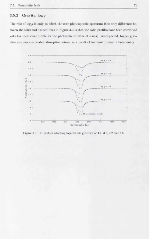
3.5.2 Gravity, l o g p ... 70
3.5.3 Mass-loss rate, M ... 71
3.5.4 Stellar radius, A * ... 72
3.5.5 Effective temperature, Tgff... 73
3.5.6 Terminal velocity, Vqo ... 74
3.5.7 Rotation velocity, u sin2 ... 75
3.5.8 Helium abundance, Y (H e )... 76
3.5.9 Equation of mass continuity... 77
3.5.10 Hydrogen and helium departure coefficients...79
4 Ha; Analyses 86 4.1 PHALTEE...86
4.1.1 The PIKAIA subroutine...86
4.1.2 M odelling ...89
4.2 Modelling the observations ... 90
4.2.1 Puls fitting p r o c e d u re ... 91
4.2.2 Equivalent w i d t h s ... 92
4.2.3 Adopted p a ra m e te rs ... 92
4.2.4 Profile f i t t i n g ...99
4.3 R esults... 100
4.3.1 Mass-loss r a t e s ...104
4.3.2 Velocity law ^ - e x p o n e n ts ... 109
4.3.3 Departure co efficien ts...110
4.4 Comparison with other s t u d i e s ... 113
4.5 E r r o r s ... 115
4.5.1 The correlation between M and / 3 ... 125
4.5.2 Com m ents... 127
Contents 10
5.2 The Sub-millimetere Common User Bolometer Array (S C U B A )...130
5.3 Data re d u c tio n ... 132
5.3.1 C a lib ra tio n ... 133
5.4 Flux d e te c tio n s ... 134
5.5 Free-free continuum e m issio n ...136
5.6 Calculating mm mass-loss r a t e s ...138
5.6.1 Distance, d ... 138
5.6.2 Terminal wind velocity, V o o... 139
5.6.3 Wind electron temperature, T g ... 139
5.6.4 Mean molecular weight, / i ... 140
5.6.5 Mean ionic charge, Z, and number of free electrons per ion, j . . . . 140
5.6.6 E r r o r s ...141
5.7 Characteristic radius of e m is s io n ... 144
6 Radio: Mass-Loss Rates 148 6.1 Published observations... 148
6.2 Spectral in d ex ...161
6.2.1 Observed spectral in d ic e s ... 162
6.3 Calculating radio mass-loss r a t e s ... 164
6.3.1 Stellar and wind param eters... 164
6.3.2 R e s u l t s ...172
6.4 Nonthermal em ission... 177
6.4.1 Observable characteristics of nonthermal emission ... 177
6.4.2 Criteria for establishing nonthermal e m is s io n ...178
6.4.3 Possible origins of nonthermal emission ... 184
6.5 Wind-wind in te ra c tio n s ... 185
6.5.1 B in a rity ...186
6.5.2 X-ray e m is s io n ... 186
6.5.3 Possible c o rre la tio n s... 187
7 Discussion and Future Work 193 7.1 Comparison of H a and radio mass-loss r a te s ...194
7.2 Wind-momentum-luminosity relationship (W L R )... 199
Contents 11
7.2.2 Observed W L R ... 201
7.3 Future w o rk ...207
A Optimised H a Line-Profile Fits 211 A .l HD 2905 (k C a s ) ... 213
A.2 HD 5394
(7
C a s ) ... 213A.3 HD 1 0 1 2 5 ... 214
A.4 HD 12323 ... 214
A.5 HD 13745 (V354 Per) ... 215
A.6 HD 14947 ... 215
A.7 HD 15558 ... 216
A.8 HD 15570 ... 216
A.9 HD 16429 ... 217
A.IO HD 30614 (a C a m )... 217
A .ll HD 34078 (AE A u r ) ... 218
A.12 HD 36486 Cri A) ... 218
A.13 HD 37742 (( C r i ) ... 219
A.14HD 66811 (C P u p ) ... 219
A.15 HD 105056 (OS Mus) ... 220
A.16 HD 123008 ... 220
A.17 HD 149038 {fi N o r)... 221
A.18 HD 149404 (V918 S c o )... 221
A.19 HD 149757 (( Oph) ... 222
A.20 HD 152003 ... 222
A.21 HD 152147 ... 223
A.22 HD 152249 ... 223
A.23 HD 152405 ... 224
A.24 HD 152424 ... 224
A.25 HD 154368 ... 225
A.26 HD 154811 ... 225
A.27 HD 156212 ... 226
A.28 HD 164794 (9 S g r ) ... 226
Contents 12
A.30 HD 167971 (MY S e r) ... 227
A.31 HD 168112 ... 228
A.32 HD 168607 ... 228
A.33 HD 169454 ... 229
A.34 HD 169515 (RY S e t ) ... 229
A.35 HD 169582 ... 230
A.36 HD 188209 ... 230
A.37 HD 189957 ... 231
A.38 HD 190429A ...231
A.39 HD 190603 ... 232
A.40 HD 191781 ... 232
A.41 HD 192281 ... 233
A.42 HD 193237 (P Cyg) ... 233
A.43 HD 194279 ... 234
A.44 HD 194280 ... 234
A.45 HD 195592 ... 235
A.46 HD 197345 (a Cyg) ... 235
A.47 HD 201345 ... 236
A.48 HD 202124 ... 236
A.49 HD 206267A ...237
A.50 HD 207198 ... 237
A.51 HD 209975 (19 C e p ) ... 238
A.52 HD 210809 ... 238
A.53 HD 210839 (A C e p )... 239
A.54 HD 214680 (10 L a c ) ... 239
A.55 HD 218195 ... 240
A.56 HD 218915 ... 240
A.57 HD 225160 ... 241
A.58 Cyg 0B2 N o . 5 ...241
A.59 Cyg 0B2 N o . 7 ...242
A.60 Cyg 0B2 N0.8A ... 242
A.61 Cyg 0B2 N o . 9 ...243
Contents 13
A.63 V433 S e t...244 A.64 MWC 349 ... 244
L
is t
o f
F
i g u r e s
1.1 Schematic diagram of the photon-scattering process ...31
1.2 Schematic diagram showing the formation of a P-Cygni p r o f i l e ...32
2.1 Spectrum of HD 149757 after bias subtraction... 40
2.2 Spectrum of HD 149757 after fiat-fielding and cosmic-ray subtraction . . . . 41
2.3 Spectrum of HD 149757 after rectification and telluric c o rre c tio n ... 41
2.4 Spectrum of HD 189957 before and after telluric c o rre c tio n ... 42
2.5 Spectrum of HD 195592, centred on the Ho: fe a tu re ...44
2.6 H-R diagram showing the location of the H a sample s t a r s ...50
2.7 Histogram showing the distribution over spectral type of the Hot sample . . 51
3.1 Observed spectrum and model photospheric H a profile of HD 210839 . . . . 59
3.2 Effect on H a of varying the velocity law yd-exponent...69
3.3 Efiect on H a of varying the g ra v ity ... 70
3.4 Effect on H a of varying the mass-loss r a t e ... 71
3.5 Effect on H a of varying the stellar r a d i u s ... 72
3.6 Effect on H a of varying the effective te m p e ratu re ...73
3.7 Effect on H a of varying the terminal v e lo c ity ... 74
3.8 Effect on H a of varying the rotation velocity ... 75
3.9 Effect on H a of varying the helium abundance ... 76
3.10 Effect on H a of varying M and R*, at constant 78 3.11 Effect on H a of varying 63“ (H) and 64“ (He) at (He) = 5 .0 ... 81
3.12 Effect on H a of varying b f (H) and 64” (He) at (He) = 1 0 . 0 ... 82
3.13 Effect on H a of varying b f (H) and b f (He) at 5g° (He) = 1 5 . 0 ... 83
3.14 Effect on H a of varying 5^ (H) and 64“ (He) at 6g° (He) = 2 0 . 0 ... 84
List of Figures 15
3.15 Effect on H a of varying 6^ (H) and b f (He) at (He) = 2 5 , 0 ... 85
4.1 Comparison of interactive and automated fits for Cyg 0B 2 No.8A ...100
4.2 PHALTEE results for HD 14947 ... 102
4.3 Mass-loss rate as a function of stellar luminosity for the entire H a sample . 107 4.4 Mass-loss rate as a function of stellar luminosity for the O s t a r s ...108
4.5 Mass-loss rate as a function of W \ ( H a ) ...108
4.6 as a function of Wx ( H a ) ... I l l 4.7 Change introduced into logM when the bi are allowed to fio a t...121
4.8 Change introduced into ^ when the 6% are allowed to f l o a t ...122
4.9 Change introduced into 63” (H) when the hi are allowed to f i o a t ...122
4.10 Change introduced into (He) when the bi are allowed to f i o a t ... 123
4.11 Change introduced into (He) when the hi are allowed to f i o a t ... 123
4.12 Correlation between AP and A lo g M ... 124
4.13 Correlation between A6g° (He) and A l o g M ...124
4.14 /3 as a function of mass-loss rate ...125
4.15 Effect on M of varying ^0, for HD 12323 ... 127
4.16 H a line-profile fits to HD 12323, for P = 0.3-2.0...128
5.1 Final, mm photometric SCUBA result for a C y g ...133
6.1 H-R diagram showing the location of the radio sample s t a r s ... 160
6.2 Histogram showing the distribution over spectral type of the radio sample . 161 6.3 Mass-loss rate as a function of stellar luminosity for the entire radio sample 183 6.4 Mass-loss rate as a function of stellar luminosity for the thermal sources . . 184
6.5 Correlation between nonthermal radio emission and excess X-ray emission . 190 7.1 Comparison of H a and radio mass-loss r a te s ... 197
7.2 Observed WLR for the O stars in the H a s a m p le ... 205
7.3 Observed WLR for the B stars in the H a sample ... 206
L
i s t
o f
T
a b l e s
1.1 MK luminosity classification s c h e m e ... 20
1.2 Representative parameters for early-type s ta r s ... 22
1.3 Walborn’s 0-type star spectral designations... 24
2.1 INT target stars ...38
2.2 WHT target s ta r s ... 45
2.3 AAT target s t a r s ...47
2.4 ( P u p ... 49
2.5 Summary of observations ... 50
3.1 Parameter ranges for the 0-star model atmosphere g r id s ...58
3.2 Parameter ranges for the B-star model atmosphere g r id s ... 58
3.3 Boundary values of the H departure coefficients, bi (z = 2 , 3 , 4 , 5 ) ... 65
3.4 Boundary values of the He II departure coefficients, hi {i = 4,6,8,10) . . . . 66
3.5 Parameter ranges for the sensitivity tests ... 68
3.6 Values of M and R* adopted (at constant M /R ^) to generate H a profiles . 78 4.1 ‘Standard’ values of ^ used in initial model f i t s ... 91
4.2 H a equivalent widths for the stellar s a m p l e ... 93
4.3 Adopted parameters for the Ha sample ... 94
4.4 Search ranges for the free PHALTEE p a ra m e te rs ... 101
4.5 Sample size of the H a data by spectral type and luminosity c l a s s ... 101 4.6 Numerical results of the PHALTEE searches conducted with the hi fioating . 103 4.7 Mean values of derived M for different spectral types and luminosity classes 105 4.8 Mean values of derived /3 for different spectral types and luminosity classes 109
List of Tables 17
4.9 Mean values of derived 6^ (H) for different spectral types and luminosity c la s s e s ...I l l 4.10 Mean values of derived 64" (He) for different spectral types and luminosity
clcisses...112
4.11 Mean values of derived (He) for different spectral types and luminosity c la s s e s ...112
4.12 Comparison of results from this work with those from Puls et al (1996) . . 114
4.13 Numerical results of the PHALTEE searches conducted with the hi fixed . . .116
4.14 Change in the PHALTEE results introduced by fioating the departure coeflS- cients ...118
5.1 SCUBA target s t a r s ... 135
5.2 Adopted parameters for the SCUBA sam p le...142
5.3 Mass-loss rates derived from SCUBA mm fluxes...145
5.4 Characteristic radii of emission for the SCUBA sa m p le ... 147
6.1 Published radio and mm detections of Galactic early-type s t a r s ...150
6.2 Adopted parameters for the radio s a m p l e ...166
6.3 Radio mass-loss ra te s ... 174
6.4 Criteria for establishing nonthermal e m is s io n ... 181
6.5 Binarity and X-ray em ission... 188
6.6 Correlation between excess radio and excess X-ray e m is s io n ... 191
6.7 Stars exhibiting excess radio and excess X-ray emission ... 192
6.8 Fisher’s exact test for binarity and nonthermal/ excess X-ray emission . . . 192
7.1 Comparison of H a and radio mass-loss r a te s ... 196
7.2 Observed wind momenta for the Ha s a m p le ...203
C h a p t e r 1
Introduction
This thesis is concerned with the physics of mass loss from hot, luminous stars. The term ‘hot star’ is used here to refer primarily to stars of spectral types O and B (effective tem perature, Tgff > 10000 K), whilst the description ‘luminous’ should be read £is excluding subdwarfs. Such objects occupy the upper left-hand corner of the Hertzsprung-Russell (H-R) diagram, and are synonymously known as massive, early-type or OB stars. All these terms will be used throughout this work.
1.1
Spectral classification
In order to organise the diversity of stellar spectra both in a tractable manner and in a way which encourages an astrophysical interpretation, stars are classified according to the appearance of their spectra. This classification is essentially a concise description of the key morphological features in the optical spectrum. Spectral classification greatly simplifies the treatment and comparison of results, and is one of the standard tools employed in the explanation of stellar evolution.
1.1.1 T he Harvard classification schem e
The core of modern spectral classification is the Harvard scheme, developed at the Har vard Observatory by Cannon and Pickering (1918) for the Henry Draper (HD) catalogue. Initially, the Harvard scheme alphabetically classified stars according to the strengths of the hydrogen Balmer lines in their spectra, with the A stars having the strongest Balmer
1.1. Spectral classification 19
lines. After some rearrangement and the omission of certain letters, the final ordering corresponded to a sequence of decreasing
temperature:-0 - B - A - F - G - K - M
Decreasing temperature
The stars near the beginning of the sequence are known as ‘early-type’ stars, and those towards the end ‘late type’ (the Harvard workers erroneously thought th at their original arrangement was an evolutionary sequence). W ithin each spectral class there are subdivisions (subtypes), denoted by a number > 0 to < 10, where the ‘0’ subtype is the hottest (the exception being the O stars, where the ‘2’ subtype is the hottest; Walborn
et al., 2002).
1.1.2 M K lu m in o sity classification
1.2. The initial mass function (IMF) 20
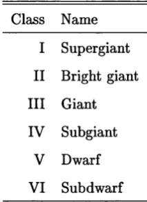
Table 1.1: The MK luminosity classification scheme
Class Name
I Supergiant
II Bright giant
III Giant
IV Subgiant
V Dwarf
VI Subdwarf
No t e: The subdwarf ‘VI’ classification is rarely used.
1.2
T he initial m ass function (IM F)
The most important factor when considering the evolution of a star is its initial mass. A star’s mass determines both its main-sequence lifetime and its contribution to the enrich ment of the interstellar medium (ISM) with heavy elements. High-mass stars dominate the luminosity of young galaxies and clusters, and are the primary source of the alpha elements, such as oxygen and magnesium. Intermediate-mass stars dominate the lumi nosity in older stellar systems, and, via Type la supernovae (SNe), are the origin of the iron-peak elements. Low-mass stars contain most of the baryonic mass which is involved in star formation. When the initial stellar mass is considered in conjunction with evolu tionary models (e.g. Schaller et al, 1992; Meynet et al, 1994), it is possible to project other stellar parameters (e.g. Tgff and luminosity) at any point during the star’s lifetime.
The initial mass function (IMF) describes the relative numbers of stars which form as a function of their main-sequence mass from a unit mass of ISM. Essentially, it describes the probability of a star forming with a given mass, and thus specifies the distribution in mass of a newly-formed stellar population. It is fundamentally important for a description of the luminosity and chemical evolution of the Universe.
1.3. Early-type stars 21
probability of a star forming with mass m , and is defined such
that:-diV = (j){m)dm (1.1)
where d N is the number of stars, per unit volume, of absolute visual magnitude in the interval. M y to (My + dM y), and (j){m)dm is the number of stars formed at the same time, per unit volume, with initial masses in the interval, m to (m + dm). The mass function is, empirically, well described by a power
law:-(j){m) = arn' (1.2)
Salpeter (1955) found an IMF slope, 7 = —2.35. This power law appears to adequately apply for stellar masses in the range 1-100 M©. Scalo (1986), however, demonstrated th at a single power law cannot reproduce the shape of the IMF over the full stellar mass range. Scale’s (1986) treatment gives a decrease in slope at low masses (observations have since confirmed this), and a steeper function relative to the Salpeter IMF at high masses (the observational case for this remains uncertain). It has been suggested (Massey, 1998) th at there is no ‘upper mass cutoflF’ to the IMF, with statistics, rather than physics, limiting the highest-mass stars th at we observe. The recent overview provided by contributions in the proceedings of the 38th Herstmonceux Conference on ‘The Stellar IM F’ (Gilmore and Howell, 1998) indicates that the stellar IMF is nearly a universal function. To a good first approximation, it would appear to apply at all metallicities, at all star formation rates, in all environments, and at all times.
1.3
E arly-type stars
1.3. Early-type stars 22
Lamers and Leitherer, 1993; Puls et al, 1996; Herrero et al, 2000, 2002), During the final stages of their evolution, as Luminous Blue Variables (LBVs), Wolf-Rayet (WR) stars and, ultimately, supernovae, they may inject vast amounts of enriched material into the ISM (see the Frontispiece for an image of the star HD 148937, which is surrounded by symmetrical shells of material, believed to have been ejected during violent mass- loss outbursts). Thus, although massive stars form only a small fraction of the stellar population within the Galaxy (because of the nature of the IMF), they play an important rôle in its evolution, both chemically and kinematically (Abbott, 1982), The properties of such objects are therefore of great interest.
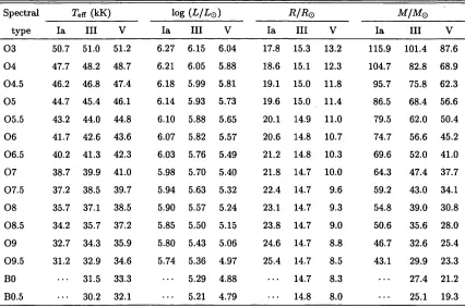
Table 1,2: Representative parameters for early-type stars
Spectral type
Teff (kK) log (L /L o) R / Rq M / Mq
la III V la III V la III V la III V
0 3 50.7 51.0 51.2 6.27 6.15 6.04 17.8 15.3 13.2 115.9 101.4 87.6 0 4 47.7 48.2 48.7 6.21 6.05 5.88 18.6 15.1 12.3 104.7 82.8 68.9 04.5 46.2 46.8 47.4 6.18 5.99 5.81 19.1 15.0 11.8 95.7 75.8 62.3 0 5 44.7 45.4 46.1 6.14 5.93 5.73 19.6 15.0 11.4 86.5 68.4 56.6 05.5 43.2 44.0 44.8 6.10 5.88 5.65 20.1 14.9 11.0 79.5 62.0 50.4 0 6 41.7 42.6 43.6 6.07 5.82 5.57 20.6 14.8 10.7 74.7 56.6 45.2 06.5 40.2 41.3 42.3 6.03 5.76 5.49 21.2 14.8 10.3 69.6 52.0 41.0 0 7 38.7 39.9 41.0 5.98 5.70 5.40 21.8 14.7 10.0 64.3 47.4 37.7 07.5 37.2 38.5 39.7 5.94 5.63 5.32 22.4 14.7 9.6 59.2 43.0 34.1 0 8 35.7 37.1 38.5 5.90 5.57 5.24 23.1 14.7 9.3 54.8 39.0 30.8 08.5 34.2 35.7 37.2 5.85 5.50 5.15 23.8 14.7 9.0 50.6 35.6 28.0 0 9 32.7 34.3 35.9 5.80 5.43 5.06 24.6 14.7 8.8 46.7 32.6 25.4 09.5 31.2 32.9 34.6 5.74 5.36 4.97 25.4 14.7 8.5 43.1 29.9 23.3
BO 31.5 33.3 5.29 4.88 14.7 8.3 27.4 21.2
B0.5 30.2 32.1 5.21 4.79 14.8 8.0 25.1 19.3
1.3. Early-type stars 23
1.3.1 O -typ e stars
O stars are the hottest and most massive of the ‘normal’, core H-bnrning stars, with effective temperatures in the range ~ 30 000-50 000 K (the upper limit is somewhat open to question at the current time) and masses in the range ~ 20-120 Mq (again, the upper limit is not well determined). They comprise the majority of stars studied in this thesis. The 0 -sta r parameters listed in Table 1.2 are taken from the empirical calibrations of Vacca et al. (1996), which were based on plane-parallel, hydrostatic, pure H/He model atmosphere analyses. These parameters are intended merely to serve as representative quantities. Newer calibrations, based on spherically expanding, line-blanketed (see §3.1.5) model atmospheres, which include the effects of mass loss, have recently been published for O-type supergiants (Crowther et al., 20026; Herrero et al, 2002; Bianchi and Garcia, 2002) and O-type dwarfs (Martins et al, 2002). These analyses yield lower effective temperatures than unblanketed studies, especially for early O-type stars (~ 4000 K lower for luminosity class V and ~8000 K lower for luminosity class I).
O stars are characterised by the lines of hydrogen (H), neutral helium (He l) and singly ionised helium (He ll) in their optical spectra; the presence of He ll in traditional classification spectra is the defining characteristic of O-type stars. The strengths of the He I and He ll lines are closely correlated with photospheric temperature; He ll increases
in strength towards earlier (hotter) types and He I decreases in strength. Indeed, within
the 0 -star domain, the primary classification criteria are the relative line ratios of He I to
Hell (which are not directly influenced by metallicity effects). The H ell A4686 Â line can be used as a luminosity indicator, being in absorption in dwarfs and emission in giants and supergiants.
1.3. Early-type stars 24
He I A4471 Â in classification-quality photographic spectra). More recently, Walborn et al.
(2002) introduced the new 0 2 and 03.5 spectral subtypes in order to accommodate the range in classification criteria afforded by high-quality digital spectra.
Table 1.3: Walborn’s O-type star spectral designations
Designation Criteria
f strong NIII 4634-41 emission, Hell 4686 emission
(f) medium N ill 4634-41 emission, no He ll 4686 emission or absorption ((f)) weak NIII 4634-41 emission, strong H ell 4686 absorption
f* NIV 4058 emission > N ill 4640 emission (03) (f*) f* plus weak H ell 4686 absorption
((£*)) f* plus strong Hell 4686 absorption
f characteristics plus Si IV 4089, 4116 emission (04-6)
f?p C m 4647-51 emission like N lll 4634-41; H P-Cyg profiles
e Balmer cores in emission
(e) probable emission at H/3
e"^ a-Cyg shell lines in emission n broad nebulous or diffuse lines (n) in between n and ((n))
((n)) Si IV 4116 and He I 4121 just merged
[n] broadening H lines He lines
nfp He II centrally reversed emission
N N III, NII absorption lines enhanced
C C III, CII absorption lines enhanced, N lines deficient
Re f e r e n c e: Divan and Prevot-Burnichon (1988).
1.3.2 B -ty p e stars
1.3. Early-type stars 25
around B2-B3) decreases. He II is absent in traditional classification spectra (but can be
detected in early-B stars by using high-quality digital spectra).
Two important subgroups of B stars are the Be and B[e] stars. These are emission-line objects that exhibit evidence for equatorially-enhanced winds (often referred to as ‘disks’). Be stars are non-supergiant B stars whose spectra show (or have shown) Baimer fines in emission (Slettebak, 1988); they are also observed often to have much stronger infrared excesses than ‘normal’ early-type stars (Allen and Swings, 1976). Possible scenarios in voked to explain the Be-star phenomenon include: a) a rotationally-enhanced stellar wind (Bjorkman and Cassinelfi, 1993); b) nonradial pulsation (e.g. Baade and Balona, 1994); and c) an interacting binary (e.g. Harmanec, 1987). Typically much more luminous than the Be stars, B[e] stars are a very heterogeneous group of B-type stars (Lamers et al., 1998) that show forbidden emission fines in their optical spectra (Allen and Swings, 1976).
1.3.3 A -ty p e supergiants
A-type supergiants are massive (~ 5-25 Mq) stars that have most probably evolved from main-sequence ~ B0-B5 stars, and have effective temperatures ranging from ~ 7500- 10 000 K. Their extreme luminosity, coupled with the fact th at the peak of their spectral energy distribution is at visual wavelengths, means they are usually the brightest (up to M y — 9) single, ‘normal’ stars observed in optical surveys of other galaxies. Their po tential as independent distance indicators through use of the wind-momentum-luminosity relationship (WLR; see §7.2) means they are of increasing interest in extragalactic astron omy (Kudritzki et al., 1995, 1999; McCarthy et al, 1997, 2001; Kudritzki, 1998). The dominant feature of an A-type spectrum is the presence of strong hydrogen Baimer fines (peaking at subtype A2); the He I fines present in earlier spectral types are absent in classification-quality spectra.
1.3.4 Lum inous B lu e V ariables (L B V s)
1.3. Early-type stars 26
constant for a given object, considering the stars’ intrinsic variability. When at photo metric visual minimum, LBVs have effective temperatures in excess of ~ 15 000-20 000 K (similar to B-type supergiants); during visual maximum this can drop to around 8000 K (similar to A-type supergiants). LBVs are believed to be in a very short-lived (< 10^ yrs) evolutionary stage, intermediate to that of 0 stars and W R stars. A vast amount of mass is lost during the LBV phase: mass-loss rates during an outburst can be as high as ~ 10“ ^-10“ ^ Mq yr“ ^, effectively removing the outer layers of the star. Indeed, LBVs are often observed to possess circumstellar material in the form of shells or ejecta nebulae. The well known LBV, rj Carinae, underwent a particularly violent outburst in 1846, tem porarily becoming visually the second brightest star in the sky. LBVs lie very close to the Humphreys-Davidson limit (Humphreys and Davidson, 1979), an observed upper luminos ity limit in the H-R diagram, above which no stars are normally seen. The outbursts may be directly related to whatever mechanism brings about the Humphreys-Davidson limit, preventing the most luminous stars from becoming red supergiants (RSGs) by allowing them to shed sufficient mass.
1.3.5 W olf-R ayet (W R ) stars
Wolf-Rayet (WR) stars are believed to be the highly evolved descendants of massive, O- type stars (>25 M©; see Crowther et al., 19956), and may be the progenitors of certain types of supernovae (types Ib/Ic; see, e.g. Chu, 2002). The idea th at WR stars are young. Population I objects is supported by the fact that they are often seen associated with OB stars in open clusters, or as binary companions to OB stars (the incidence of binarity amongst WR stars is high; e.g. van der Hucht, 2001). Their original outer layers have previously been lost through strong stellar winds (either continuously or in outbursts associated with the LBV phase), revealing the products of interior nuclear processing at their surfaces. WR stars are observed to be hydrogen deficient, and are characterised by strong, broad emission lines of ionised He, N, C and O in their spectra. These lines originate in their powerful, optically thick stellar winds, which typically have velocities in the range ~ 1000-4000 km s“ ^. The winds drive mass-loss rates of order ~ 10“ ^ Mq yr“ ^.
WR stars have extremely high elective temperatures, typically in the range ~ 30000- 90000 K (to the extent that Teff can be defined for such objects).
1.4- Mass loss 27
no nitrogen); and the rare WO stars (oxygen spectra dominant, the ratio C /0 < 1). The WN stars appear to exhibit the products of CNO-cycle buring, whereas the more evolved WC and WO stars show the products of helium burning and a-capture. The spectral classification of OB stars is closely coupled to stellar effective temperature and luminosity; however, in the case of WR stars, the classification is based mainly upon the emission- line ratios of ions of He, N, C and 0 , formed in an optically thick stellar wind, WR spectral types, therefore, give only an approximate indication of the temperature and ionisation in WR winds. The WR classification scheme allows for the following spectral subtypes: WN2-WN11, WC4-WC9 and W 01-W 04 (see van der Hucht, 2001, for a review of the classification criteria for WR stars). Crowther et al. (19956) proposed the following evolutionary scenarios for massive stars, dependent upon initial stellar mass,
Mf.-(i) O Of ^ WNL -4. WN7 ( ^ WNE) WC -> SN for M* > 60M©
(ii) O - 4 Of-)- LBV 44 WN9-11 - 4 WN8 -> WNE - 4 WC -> SN for 40M© < M* < 60M© (iii) O -4- Of -> RSG -> WN8 -4- WNE - 4 WC -> SN for 25M© < M* < 40M©
where WNE and WNL refer to ‘early-’ (WN2-5) and ‘late-type’ (WN6-11) WN stars, respectively. Thus, W R stars are crucially important to our understanding of the final stages of massive-star evolution.
1.4
M ass loss
As stated previously, throughout most of their lives, early-type stars continually lose mass by way of strong stellar winds (e.g. Abbott et al, 1981). A stellar wind is a (more or less) continuous outfiow of material from the outer layers of a star into the ISM. All stars lose mass, but the mass-loss rates depend greatly upon the type of object concerned. The sun (spectral type G2V) sheds mass at a rate of M© yr“ ^, thus losing a negligible amount of material over a Hubble time. A typical O star, however, with a mass-loss rate in the region of ~ 10“ ^-10“ ® M© yr~^, will lose a few solar masses during its main-sequence lifetime. Being a significant fraction of the initial stellar mass, this ‘evaporation’ has a number of important consequences.
1.4- Mass loss 28
massive star (e.g. OB stars, LBVs, WR stars; see Langer et a/., 1994). Secondly, as a result of the outer envelopes being stripped away, CNO-processed material may be exposed at the stellar surface; these products are observable spectroscopically and can be used as a test of stellar evolution. Also, because of its effect on the stellar interior, mass loss influences the nature of supernovae precursors. Thirdly, through the deposition of nucleosynthetically enriched material, momentum and energy, the wind ejecta have an impact on the nature of the ISM (e.g. Abbott, 1982). In addition to these important consequences, the presence of a wind may also affect the emergent stellar spectrum, which in turn can influence a star’s spectral classification. For these reasons, the study of mass loss from hot, luminous stars is of considerable interest and warrants quantitative analysis.
1.4.1 Fundam ental con cep ts
Massive-star winds are driven by radiation: ions in the wind are ‘pushed out’ from the star by the scattering of photons in spectral lines. The opacity of one strong line can be as much as ~ 10® larger than the electron-scattering opacity. However, the large radiation force on the ions would not be efficient were it not for the Doppler effect. In a static atmosphere with strong line absorption, radiation would be absorbed and scattered in the lower layers, meaning that the outer layers would not receive photons at the line frequency. In a radially-expanding atmosphere (e.g. a stellar wind), the presence of a velocity gradient allows the ions to ‘see’ photospheric radiation as red-shifted. Thus, ions in the outer atmosphere are able to absorb unattenuated radiation from the photosphere. It is for this reason that radiative acceleration is a very efficient mechanism for driving stellar winds. Material escaping from the outer layers of a star is monotonically accelerated outwards (in the case of a smooth wind) from a small velocity (typically v < 1 km s“ ^) at the stellar photosphere, to some high velocity at a large distance from the star. The modern version
of radiation-driven wind theory was developed by Lucy and Solomon (1970) and Castor
et al (1975).
Motivated by rocket-based observations of the UV spectra of OB supergiants (Morton, 19676, and subsequent papers), UV spectroscopy from the Copernicus and International
Ultraviolet Explorer (lUE) satellites has shown mass loss to be a ubiquitous character
1.4- Mass loss 29
stellar mass loss th at can be derived from observations, are the mass-loss rate, M , and the terminal velocity of the wind, Voo- M and Vqo are important
because:-(i) The value of M greatly affects stellar evolution (e.g. Chiosi and Maeder, 1986; Meynet et a/., 1994).
(ii) Different theories of stellar winds predict different values of M and Uqo- By compar ing observations with model predictions, it is possible to learn which mechanism is responsible for driving mass loss and the wind acceleration.
(iii) Material escaping from a star carries with it chemical enrichment, kinetic energy and momentum into the ISM. A knowledge of the value of permits an investigation of the effects of stellar winds on the ISM (Abbott, 1982).
Mass-loss rates of order ~ 10“ ® M© yr“ ^ are not unusual for early-type stars (e.g. Puls
et al, 1996; Herrero et al, 2000, 2002), and the most massive O stars can have terminal
velocities in excess of 3000 km s“ ^ (e.g. Howarth et al, 19976).
For a star with a spherically symmetric, steady and homogeneous wind, M is related to the density, p, and velocity, v, at any point in the wind
via:-M = 4:Trr^ p{r)v{r) (1.3)
where r is the radial distance measured from the centre of the star. This equation states th at material is neither destroyed nor created in the wind (i.e., it is the equation of mass continuity). The distribution of the velocity of the wind with radial distance from the star is known as the velocity law, v{r). The numerical realisation of the original version of radiation-driven wind theory (Ccistor et al, 1975) assumed the star to be a point source of radiation, and predicted a velocity law
of:-^(r) = Uoo ^1 - (1.4)
1.5. Mass-loss diagnostics 30
et al. (1986). Relative to the winds of cool stars, /? = 0.8 corresponds to a fast acceleration,
with the wind reaching 80% of its terminal velocity at r = 4.1 R* (i.e., 3.1 R* above the stellar photosphere). In general, the parameterisation given in Equation 1.4 (with varying values of /3) provides a useful characterisation of accelerating outflows, and in particular is a fair description of most subsequent models and observations.
1.5
M ass-loss diagnostics
There are a number of spectroscopic and continuum diagnostics available that can be used to estimate M , Vqq, or both, including: a) P-Cygni profiles of UV resonance lines; b) radio and IR continuum emission; and c) emission lines, especially Ho;. These reflect, respectively, bound-bound, free-free and free-bound processes.
1.5.1 U V P -C y g n i profiles
The most sensitive indicators of mass loss are the spectral lines due to atomic transitions from the ground state (known as resonance transitions) of abundant ions in the stellar wind. The resonance hnes of many atoms and ions abundant in 0 -star winds are located in the UV region of the spectrum (A < 2000
A).
Commonly used examples in the spectra of early-type stars include the resonance-line doublets of C iv (AA1550A),
N v (AA1240A)
and SiIV (AA1400A).
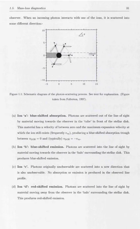
Because of the outflowing nature of the wind, the relatively high abundance of these ions (together with the large oscillator strengths of their resonant tran sitions) produces a blue-shifted absorption component and a red-shifted emission compo nent. The Doppler shifts give the lines a characteristic shape, known as a P-Cygni profile (named after the first star in which this type of profile was observed). The formation of a P-Cygni profile can be explained qualitatively by considering the contributions from different regions of the stellar envelope.1.5. Mass-loss diagnostics 31
observer. When an incoming photon interacts with one of the ions, it is scattered into some different
direction:-o b s e rv e r
- 5
-- 1 0
- 5 0 5 10 15
Figure 1.1: Schematic diagram of the photon-scattering process. See text for explanation. (Figure taken from Fullerton, 1997).
(a) Ion ‘a ’: b lu e-sh ifted a b so rp tio n . Photons are scattered out of the line of sight by material moving towards the observer in the ‘tube’ in front of the stellar disk. This material has a velocity of between zero and the maximum expansion velocity at which the ion still exists (frequently Uqo), producing a blue-shifted absorption trough between îilos = 0 and (typically) u lo s =
~Voo-(b) Ion ‘b ’: b lu e-sh ifted em ission. Photons are scattered into the line of sight by material moving towards the observer in the ‘halo’ surrounding the stellar disk. This produces blue-shifted emission.
(c) Ion ‘c’. Photons originally unobservable are scattered into a new direction that is also unobservable. No absorption or emission is produced in the observed line profile.
1.5. Mass-loss diagnostics 32
A b s o r p t i o n 1 . 5
-E m i s s l o n 1 . 5
0 . 5
-1 . 5 - P C y g = A + E
1.0
- 0 . 5 0 .5
1.0 0.0 1.0 1.0 0 .5 0.0 0 .5 1.0
Vlos / V. Vl o s / V o
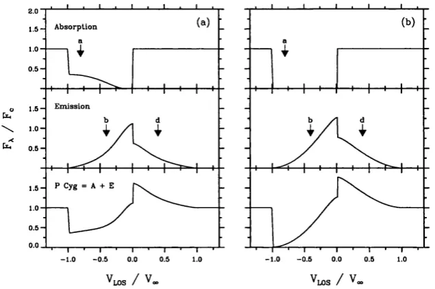
Figure 1.2: Schematic diagram showing the formation of a P-Cygni profile of a UV resonance line, for the case of: (a) a moderately strong line; and (b) a strong line. (Figure taken from Fullerton,
1997).
There is also continuum emitted from the stellar photosphere (possibly with a photo- spheric absorption component at the rest wavelength of the line concerned). When added together, these different contributions result in a P-Cygni profile, with its characteristic blue-shifted absorption trough and red-shifted emission lobe. This is illustrated in Fig ure 1.2, where the photons scattered by ions ‘a’, ‘b ’ and ‘d’ are mapped to positions in the observed line profile. The ratio of the emission strength to the absorption strength depends upon the size of the region in which the scattering occurs, relative to the size of the star. If the stellar disk is small (i.e., pointlike) compared to the size of the scattering region and emits only continuum, no radiation is lost by back-scattering into the star. In this case, and if the line is formed purely by scattering, the emission is equal to the absorption (since photon numbers are conserved).
1.5. Mass-loss diagnostics 33
measured to an accuracy of order 100 km s“ ^. Care must be taken, however, as Uobs does not (in general) equal the terminal velocity, Vqq. If the winds are at all turbulent, or have
non-monotonic velocity laws, then the maximum flow velocity, Umax, will normally exceed
Voo’ In sufficiently saturated lines, it is expected that Uobs ~ ^max ^
^oo-A widely observed phenomenon in the unsaturated P-Cygni profiles of OB stars are narrow absorption features (Snow, 1977; Prinja and Howarth, 1986). These take the form of distinct dips in the P-Cygni profile, typically seen as broad, low-velocity optical depth enhancements, which migrate (within the profile) to become high-velocity, narrow absorption features (Prinja et o/., 1987; Prinja and Howarth, 1988). Howarth and Prinja (1989) suggested that the central velocity of narrow absorption features might provide a better indicator of Uqo than does Uobs, and noted that the maximum velocity of fully saturated absorption gives a similar value.
Determining the mass-loss rate from UV P-Cygni profiles requires a knowledge of the fractional abundances of the ions concerned (Howarth and Prinja, 1989; Kudritzki et al.,
1999; Herrero et al., 2001). Because resonance lines are produced by minority ions in the wind, these fractions are small and poorly known (e.g. Groenewegen and Lamers, 1991). Another problem is that there is a limited dynamical range; lines are often very optically thick or thin, whereas only intermediate optical depths are useful. These facts, along with the need for satellite observations, limit the use of UV P-Cygni profiles in stellar-wind studies. Nevertheless, useful work can still be done: UV spectra obtained with the Hubble
Space Telescope (HST) and Far Ultraviolet Spectroscopic Explorer (FUSE) have been used
to determine the parameters of massive stars in the Magellanic Clouds (Crowther et al.,
2002a,6), M31 (Bresolin et al, 2002) and M33 (Urbaneja et a l, 2002).
1.5.2 R adio and IR continuum em ission
As a result of free-free processes, an ionised stellar wind emits continuum emission, which, because of the diminishing relative importance of the photospheric emission, is most easily observed from IR to radio wavelengths. Assuming that the wind is steady, and given that the emission is thermal in origin, observations of the radio continuum flux should provide the most accurate and reliable method for determining the mass-loss rate from an early- type star (e.g. Abbott et al, 1980, 1981; Leitherer and Robert, 1991; Leitherer et al, 1995; Scuderi et al, 1998).
1.5. Mass-loss diagnostics 34
where the outflow has reached its terminal velocity. Thus, acceleration eflects do not have to be taken into consideration when interpreting the data, and a simple r~^ density distribution can be used to describe the outflow. Provided th at the radio emission is thermal in origin (i.e., produced by free-free radiation in the outer part of the wind), then the mass-loss rate is simply related to the measured flux, the star’s distance, and the terminal velocity of the wind (see §5.5, Equation 5.2; Wright and Barlow, 1975; Panagia and Felli, 1975). This method of determining mass-loss rates is virtually independent of abundances, and of details of ionisation fractions of metals. In §5 and §6, mm and cm continuum emission will be used to derive mass-loss rates for a sample of Galactic early-type stars.
There are, however, a number of drawbacks to using radio continuum
emission:-(i) The number of early-type stars with accurate measurements in the radio is small. This is because the large distances of these objects and the intrinsic weakness of the emission conspire to make flux densities at radio wavelengths rather low (typically less than a few mJy). Generally, only higher-luminosity objects have stellar winds strong enough to be detected.
(ii) Distances to sources need to be known.
(iii) UV or other observations are required to give Voo (this is true for all diagnostics of M). Measurements of Vqq in UV resonance lines, which represent the outflow at ~ 10 i?*, are usually extrapolated to the radio-emitting region of the wind, assuming a constant outflow velocity.
(iv) Free-free emission is a density-squared (p^) process, and is therefore sensitive to clumping in the wind (Abbott et al, 1981). The presence of structure within a density distribution that is assumed to be smooth will cause M to be overestimated when using Equation 5.2 (see §7.1).
(v) Many OB stars are observed to be sources of nonthermal radio emission (Bieging
et al, 1989; Altenhoff et a l, 1994). This contaminates (and can indeed dominate)
the free-free emission, invalidating the use of Equation 5.2 to calculate mass-loss rates.
1.5. Mass-loss diagnostics 35
density structure in the inner part of the wind. Nevertheless, IR emission is a useful probe of conditions nearer the star, in the region where the outflow is still undergoing acceleration.
1.5.3 E m ission lines
Early-type stars with mass-loss rates in excess of ~ 10“ ® Mq yr“ ^ show broad, wind-
formed emission lines in their spectra, particularly those of H, He I and He II. The best known, and typically the strongest of these, is H a (A6563 Â). The strength and shape of the H a proflle can provide information about both M and the velocity law of the wind (e.g. Puls et al, 1996). If the wind is optically thin for a line transition (and this is often approximately valid for Ha), the mass-loss rate can be derived directly (and accurately) from the total luminosity of the line, given th at Vqo is known. The height and width of the central part of the line proflle can be used to constrain the ^-exponent of the velocity law. H a has been used to determine mass-loss rates for a variety of hot stars (e.g. Leitherer, 1988a; Scuderi et al, 1992; Lamers and Leitherer, 1993; McCarthy et al, 1997; Kudritzki
et al, 1999); the techniques employed will be discussed further in §3.3 and §3.4, and, in
§4, the H a line will be used to derive mass-loss rates for a sample of 64 Galactic early-type stars.
1.6. Overview of thesis 36
1.6
O verview o f th esis
This thesis aims to provide a general enquiry into the physics of mass loss from hot, luminous stars.
In §2, the observational considerations and data reduction of the Ho spectroscopy of 64 Galactic early-type stars are presented. The observations described were acquired using the telescopes of the Isaac Newton Group (ING) and the Anglo-Australian Observatory (AAO). In §3, the FORSOL code developed by Puls et al. (1996) is introduced. FORSOL is a very fast, approximate method of modelling the H a profiles of O stars, in order to determine their mass-loss rates (and, in certain instances, velocity field /0-exponents). Sen sitivity tests are performed to investigate how a FORSOL-calculated H a profile is affected by different stellar and wind parameters. In §4, a new program, p h a l t e e, is introduced,
which searches within a specified parameter space for the ‘best’ (quasi-least-squaxes) FOR SOL fit to an observed H a profile. This renders H a modelling both more objective and automated, while minimising the necessity for manual intervention, p h a l t e e is used to model quantitatively the H a profiles of, and thereby derive M and /0 for, the datasets presented in §2.
Ch a p t e r 2
H a: Observations and D ata Reduction
H a observations of 64 Galactic early-type stars were obtained over the years 1992-2000, using the telescopes of the Isaac Newton Group (ING) on the island of La Palma, and the Anglo-Australian Observatory (AAO) at Siding Spring, Australia.
2.1
IN T observations
Ha spectroscopy of 30 Galactic early-type stars was obtained using the Intermediate Dis persion Spectrograph (IDS) on the 2.5-m Isaac Newton Telescope (INT), a part of the ING. The observations were made by I. D. Howarth and the author on the nights of July 17th and 18th, 2000.
2.1.1 T h e sam ple
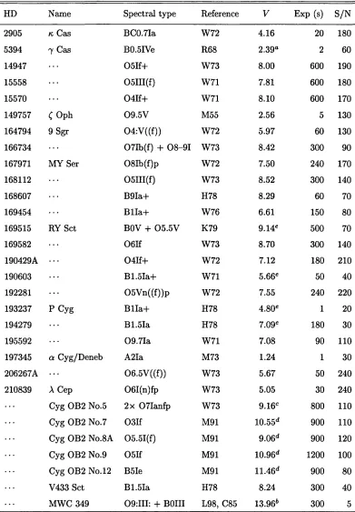
The target stars listed in Table 2.1 were selected to include objects with published radio fluxes, with a view to comparing mass-loss diagnostics (see §7.1). The sample comprises nineteen O stars, ten B stars and one A supergiant (HD 197345/a Cyg). a Cyg (commonly known as Deneb) is exceptional for its spectral type in having measurable flux at radio and mm wavelengths, and detectable H a emission. There is a bias in the sample towards supergiants (a consequence of the requirement that the targets have measurable radio emission), with 21 stars of luminosity class I, three of luminosity class HI, one of luminosity class IV and flve of luminosity class V. The V magnitudes of the sample range from 1.24 (a Cyg) to 13.96 (the ‘A’ component of MWC 349). Figure 2.6 shows the location of the sample in the H-R diagram.
2.1. IN T observations 38
Table 2.1: INT target stars
HD Name Speetral type Referenee V Exp (s) S/N
2905 K Cas BC0.7Ia W72 4.16 20 180
5394 7 Cas B0.5IVe R68 2.39“ 2 60
14947 05If+ W73 8.00 600 190
15558 05111(f) W71 7.81 600 180
15570 04If+ W71 8.10 600 170
149757
C Oph
09.5V M55 2.56 5 130164794 9 Sgr 04:V((f)) W72 5.97 60 130
166734 07Ib(f) + 08-91 W73 8.42 300 90
167971 MY Ser 08Ib(f)p W72 7.50 240 170
168112 05UI(f) W73 8.52 300 140
168607 B9Ia+ H78 8.29 60 70
169454 Blla+ W76 6.61 150 80
169515 RY Set BOV + 05.5V K79 9.14® 500 70
169582 06If W73 8.70 300 140
190429A 04If+ W72 7.12 180 210
190603 B1.5Ia+ W71 5.66^ 50 40
192281 05Vn((f))p W72 7.55 240 220
193237 P Cyg Blla+ H78 4.80® 1 20
194279 B1.5Ia H78 7.09® 180 30
195592 09.7Ia W71 7.08 90 110
197345 a Cyg/Deneb A2Ia M73 1.24 1 30
206267A 06.5V((f)) W73 5.67 50 240
210839 A Cep 06I(n)^ W73 5.05 30 240
Cyg 0B2 No.5 2x 07Ianfp W73 9.16® 800 110
Cyg 0B2 No.7 03If M91 10.55'^ 900 110
Cyg 0B2 N0.8A 05.51(f) M91 9.06"^ 900 120
Cyg 0B2 N0.9 05If M91 10.96*^ 1200 100
Cyg 0B2 N0.I2 B5Ie M91 11.46^^ 900 80
V433 Set B1.5Ia H78 8.24 300 40
MWC 349 09:111: + BOIII L98, C85 13.96** 300 5
2.1. IN T observations 39
No t e s t o Ta b l e 2.1: The Cyg 0B 2 stars are referred to by their designation number from Schulte’s
(1958) list, given that these names are in common use in the literature.
Spectral types are from: M55 — Morgan et al. (1955); R68 — Racine (1968); W71 — WaJborn (1971); W72 — Walborn (1972); M73 — Morgan and Keenan (1973); W73 — Walborn (1973); W76 — WaJborn (1976); H78 — Humphreys (1978); K79 — King and Jameson (1979); C85 — Cohen et al. (1985); M91 — Massey and Thompson (1991); L98 — Lamers et al. (1998).
0-star V magnitudes are from Garmany’s unpublished catalogue of O stars. B-star V magnitudes (along with that for a Cyg) are from Humphreys (1978), except for: a) Humphreys’ field star catalogue; b) Cohen et al. (1985) — the value listed is the mean continuum V magnitude of the ‘A ’ component; c) Torres-Dodgen et al. (1991); d) Massey and Thompson (1991); e) the on-line s im b a d astronomical database.
The sixth column gives the exposure time in seconds. Signal to noise is calculated for a small spectral region between 6440 and 6490 Â.
2.1.2 T h e In term ed iate D isp ersion Spectrograph (ID S)
The IDS is a long-slit spectrograph mounted at the Cassegrain focal station of the INT. It is equipped with two cameras, of focal lengths 235 and 500 mm; the observations presented in this thesis were made with the 500-mm camera. This was used in conjunction with an R1200R grating (i.e., a ruling of 1200 linesmm"^) to give a dispersion of 15.5 Â m m “ ^ at the detector. The detector used was a Tektronix 5 (TEK 5) CCD. This chip has a pixel size of 24 /^m, giving a maximum possible spectral resolution of 0.74 Â FWHM (corresponding to two pixels on the detector); all spectra were obtained using a slit width of 1.0", giving a resolution element of around 48 fj,m at the detector (2.0 x 24 /im pixels). This corresponds to a resolving power, R = A/A A ~ 9000 (a resolution of ~ 3 4 km s“ ^). The spectra were centred at the wavelength of the Ho: feature (6563 Â), with complete spectral coverage from roughly 6327-6727 Â. One exposure was normally obtained for each target, with exposure times ranging from 1-1200 s. The signal to noise achieved ranged from 5 to 240, with an average of ~ 120 (calculated for a small spectral region between 6440 and 6490
A).
2.1.3 D a ta red u ction
2.1. IN T observations 40
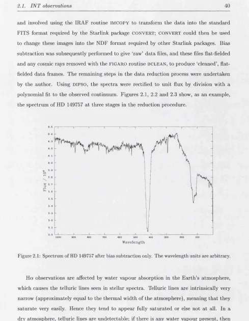
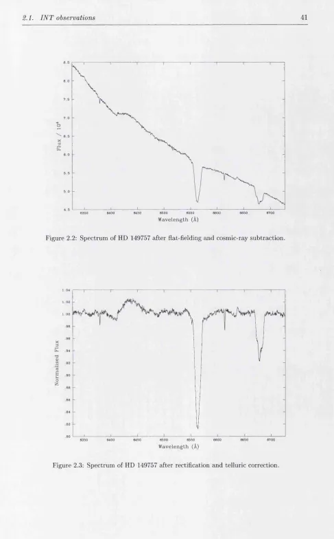
and involved using the IRAF routine IM COPY to transform the data into the standard FITS format required by the Starlink package CONVERT; CONVERT could then be used to change these images into the NDF format required by other Starlink packages. Bias subtraction was subsequently performed to give ‘raw’ data files, and these files flat-fielded and any cosmic rays removed with the FIGARO routine BCLEAN, to produce ‘cleaned’, flat- fielded data frames. The remaining steps in the data reduction process were undertaken by the author. Using DIPSO, the spectra were rectified to unit flux by division with a polynomial fit to the observed continuum. Figures 2.1, 2.2 and 2.3 show, as an example, the spectrum of HD 149757 at three stages in the reduction procedure.
6 . 5 6 . 4 6 . 3 6 . 2 6. 1
6.0
5 . 9
O
5 . 8 X 5 . 7
5: a . 6 5 . 5 5 . 4 5 . 3 5 . 2 5 . 1 5 . 0
1 000 9 0 0 BOO 7 0 0 6 0 0 5 0 0 4 0 0 3 0 0 200 100 Wavelength
Figure 2.1: Spectrum of HD 149757 after bias subtraction only. The wavelength units are arbitrary.
2.1. IN T observations 41
7 . 5
O
5 . 0
6 3 5 0 6 4 0 0 6 4 5 0 6 5 0 0 6 5 5 0 6 6 0 0 6 6 5 0 6 7 0 0
Wavelength (A)
Figure 2.2: Spectrum of HD 149757 after fiat-fielding and cosmic-ray subtraction.
1 . 0 0
6 5 5 0 6 6 0 0 6 6 5 0 6 7 0 0 6 3 5 0 6 4 5 0 6 5 0 0
Wavelength (A)
2.2. WHT observations 42
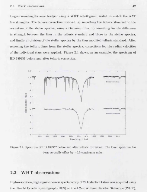
longest wavelengths were bridged using a WHT echellogram, scaled to match the AAT line strengths. The telluric correction involved: a) smoothing the telluric standard to the resolution of the stellar spectra, using a Gaussian filter; b) correcting for the difference in strength between the lines in the telluric standard and those in the stellar spectra; and finally c) division of the stellar spectra by the thus modified telluric standard. After removing the telluric lines from the stellar spectra, corrections for the radial velocities of the individual stars were applied. Figure 2.4 shows, as an example, the spectrum of HD 189957 before and after telluric correction.
X
ê
X )(U
^ 6 15
1 ^ 2
_L ± ± 6 5 4 0 6 5 5 0 6 5 6 0 6 5 7 0
Wavelength (Â)
Figure 2.4: Spectrum of HD 189957 before and after telluric correction. The lower spectrum has been vertically offset by —0.5 continuum units.
2.2
W H T observations
2.2. W HT observations 43
2.2.1 T h e sam ple
These data were acquired originally with a view to performing a differential fine spectro scopic analysis (in particular looking for object-to-object variations in the helium abun dance of O stars). Hence a large sample of objects populating a small part of the H-R diagram was desirable (see Figure 2.6). In order to obtain the required number of high- quality spectra, one of the main criteria for target-star selection was brightness: the V
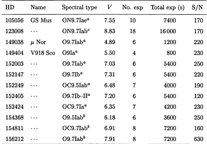
magnitudes of the sample range from 1.75 for HD 37742 (^ Ori) to 9.54 for HD 191781. Ad ditionally, a number of stars classified as OC and ON by Walborn (1976) were included, with a view to investigating possible evolutionary sequences. Table 2.2 lists the target stars. The sample comprises solely late-type O stars (spectral types 0 8 -0 9.7 ). There are twelve stars of luminosity class I, four of luminosity class II, two of luminosity class HI, and four of luminosity class V.
2.2.2 T h e U trech t E chelle Spectrograph (U E S)
2.2. WHT observations 44
1 . 5 0 1 . 4 5 1 . 4 0 1 . 3 5
X 3 E 1 . 2 0
(0
B 1- 10 O
Z 1 . 0 5
6 4 8 0 6 5 0 0 6 5 2 0 6 5 4 0 6 5 6 0 6 5 6 0 6 6 0 0 6 6 2 0 6 6 4 0
Wavelength (A)
Figure 2.5: Spectrum of HD 195592, centred on the H a feature at 6563 Â. Note the large inter-order gaps. Ha is saturated in this case, as the data were acquired originally with a view to performing an absorption-line analysis, making it necessary to obtain good signal to noise in the continuum. Scattered light from the strong emission may have caused the small features at ~ 6480 and 6640 Â in the adjacent orders. HD 195592 is the only star in the WHT sample to be affected by such
2.2. W HT observations 45
Table 2.2: WHT target stars
HD Name Spectral type V No. exp Total exp (s) S/N
10125 09.711“ 8.22 2 2700 150
12323 0N9W 8.90 2 2400 200
13745 V354 Per 09.7H((n))“ 7.88 2 1500 90
16429 09.5H((n))" 7.67 2 1500 110
30614 a Cam 09.5Ia“ 4.26 2 100 220
34078 AE Aur 09.5V“ 5.81 2 350 210
36486 Ô Ori A 09.511'’ 2.20 2 10 110
37742 (O ri 09.7Ib“ 1.75 3 19 200
188209 09.5Iab'’ 5.64 3 400 180
189957 09.5111“ 7.22 2 1000 200
191781 ON9.7Iab'’ 9.54 2 2500 110
194280 OC9.7Iab'’ 8.39 2 3000 120
195592 09.7Ia“ 7.08 2 500 80
201345 0N9V'’ 7.66 3 3000 160
202124 09.5Iab“ 7.80 2 1000 90
207198 09Ib-Il'’ 5.96 3 600 100
209975 19 Cep 09.5Ib“ 5.11 3 300 140
210809 09Iab“ 7.55 2 1000 170
214680 10 Lac 09V“ 4.87 3 150 70
218195 09111“ 8.34 2 1400 120
218915 09.5Iab'’ 7.18 3 3000 150
225160 08Ib(f)“ 8.19 2 2000 150