Scholarship@Western
Scholarship@Western
Electronic Thesis and Dissertation Repository
11-2-2016 12:00 AM
Individual Differences in Stress and Coping: Testing a Model of
Individual Differences in Stress and Coping: Testing a Model of
Decisional Control
Decisional Control
Bryan D. Grant
The University of Western Ontario
Supervisor
Dr. Richard W.J. Neufeld
The University of Western Ontario Graduate Program in Psychology
A thesis submitted in partial fulfillment of the requirements for the degree in Master of Science © Bryan D. Grant 2016
Follow this and additional works at: https://ir.lib.uwo.ca/etd
Part of the Cognitive Psychology Commons, and the Quantitative Psychology Commons
Recommended Citation Recommended Citation
Grant, Bryan D., "Individual Differences in Stress and Coping: Testing a Model of Decisional Control" (2016). Electronic Thesis and Dissertation Repository. 4206.
https://ir.lib.uwo.ca/etd/4206
This Dissertation/Thesis is brought to you for free and open access by Scholarship@Western. It has been accepted for inclusion in Electronic Thesis and Dissertation Repository by an authorized administrator of
i
Quantifying the processes of coping is one way to make the concept both descriptive and
testable. Decisional Control (DC) is a formal, mathematically-specified, normative model
which prescribes that an individual faced with a variety of alternatives in a stressing situation
will attempt to minimize objective and perceived threat of an adverse event inherent within
their choices. In this study, a game-theoretic probability mixture model created for DC was
evaluated using established indexes of model fit to empirical decision and choice data.
Sources of empirical departure from the fully normative model predictions, notably
individual and group cognitive mapping of choice linked threat, were investigated in part
through the use of psychometrical profiling of individual differences. Results of a repeated
measures ANOVA showed that individualized mappings of subjective threat significantly
improved model fit over that of the consensual and objective mappings. Additionally,
psychometric profiling did not identify notable trends in model operation.
Keywords
ii
Acknowledgments
I would like to thank my supervisor Dr. Richard W. J. (Jim) Neufeld; your guidance,
patience, and support has been a major factor in my success during the past two years of my
master’s degree. Your extraordinary support during the thesis process will always be
remembered and appreciated.
Thanks are also extended to Dr. Matthew Shanahan, Peter Nguyen, and Colleen Cutler who
helped welcome me to the research lab and acclimate me to the research we conduct. Your
kindness, jovialness, and assistance will always be gratefully remembered.
To my research assistants Melanie, Nathan, Sabrina, and Kennedy, your help and dedication
were truly paramount. This research could not have happened without your effort and time.
To my fellow colleagues, each of you have made these last few years the best they could be
with your continued encouragement, comradery and friendship. I look forward to years to
come with you all, Erin, Daniel, Kimberly, Christian, Michal, Brian, Katerina, Nadia,
Kathleen, Rhonda, Evan, Alyssa and many more.
To those in my life who have supported me from near and afar, I appreciate it every day. I
will always cherish our friendships and your faith in me, Karen, Doug, Chris, Nathan,
Jennifer, Keelan, and Nicole.
This project was helped through the support of the Western Graduate Research Scholarship
iii
Table of Contents
Abstract ... i
Acknowledgments... ii
Table of Contents ... iii
List of Tables ... vi
List of Figures ... vii
List of Appendices ... viii
Chapter 1 : Decisional Control: A Normative Model of Coping with Stress ... 1
1.1 Introduction ... 1
1.2 Normative Decision Theory ... 2
1.2.1 Multi-attribute utility (MAU). ... 3
1.2.2 Bayes’ theorem of probability theory. ... 4
1.2.3 Maximization of expected utility (Max EU). ... 5
1.3 Decisional Control ... 6
1.4 Environmental Framework of Decisional Control ... 6
1.5 Mixture Modelling ... 12
1.6 Model Testing and Fit ... 13
1.7 Aim of Current Research ... 16
Chapter 2 : Methodology ... 18
2.1 Participants ... 18
2.2 Inclusion Criteria ... 18
2.3 Exclusion Criteria ... 18
2.4 Apparatus ... 18
2.4.1 Cognitive research platform. ... 18
2.4.2 Psychometric research platform. ... 19
iv
2.5 Measures ... 19
2.5.1 Desirability of Control. ... 20
2.5.2 Need for Cognition. ... 20
2.5.3 Intolerance of Uncertainty Scale. ... 21
2.5.4 Uncertainty Tolerance Scale. ... 21
2.5.5 General Decision-Making Style. ... 22
2.5.6 Endler Multidimensional Anxiety Scale – Trait scale. ... 22
2.5.7 Probability Rating sheet. ... 23
2.5.8 Rank Ordering sheet. ... 23
2.6 Procedure ... 23
2.6.1 Measures phase. ... 23
2.6.2 Learning phase. ... 23
2.6.3 Practice phase. ... 26
2.6.4 Testing phase. ... 27
Chapter 3 : Results ... 29
3.1 DC Model Testing ... 29
3.1.1 Indication that learning occurred and participant removal. ... 29
3.1.2 Data cleaning procedures. ... 30
3.1.3 Subjective utilities of ti values. ... 31
3.1.4 G2 and Pearson χ2 calculations. ... 32
3.1.5 Outliers, normality, and transformation. ... 32
3.1.6 Repeated measures one-way ANOVA. ... 33
3.1.7 Canonical correlations. ... 34
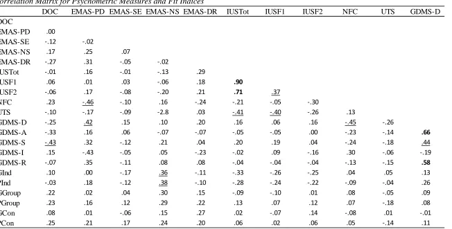
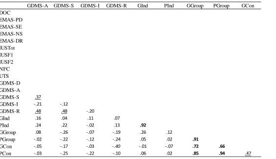
3.2 Psychometric Data ... 37
v
3.2.2 Need for Cognition. ... 38
3.2.3 Intolerance of Uncertainty. ... 38
3.2.4 Uncertainty Tolerance Scale. ... 38
3.2.5 General Decision-Making Style. ... 38
3.2.6 Endler Multidimensional Anxiety Scale – Trait scale. ... 39
3.2.7 Fit indices. ... 39
3.2.8 Correlations. ... 39
3.2.9 Canonical correlations. ... 41
Chapter 4 : Discussion ... 41
4.1 Discussion for the Primary Purpose of the Study ... 41
4.2 Discussion for the Secondary Purpose of the Study. ... 46
Chapter 5 : Conclusions ... 48
References ... 49
Appendices ... 54
vi
List of Tables
Table 1: Letters for Stimulus Presentation (During Learning and Testing phases) and
Associated Frequencies and Probabilities ... 25
Table 2: Conditional and Group Rank Orderings and Probabilities of Letter Presentations .. 32
Table 3: Descriptive Statistics for the Fit Indices by Model ... 39
Table 4: Correlation Matrix for Psychometric Measures and Fit Indices ... 39
vii
List of Figures
Figure 1: An example of a nesting-nested hierarchy (decision tree) with ti elements
randomized at the most subordinate level ... 7
Figure 2: A simplified graphical representation of the hypothetical relationship between
cognitive processing and the probability of experiencing an adverse-event ... 10
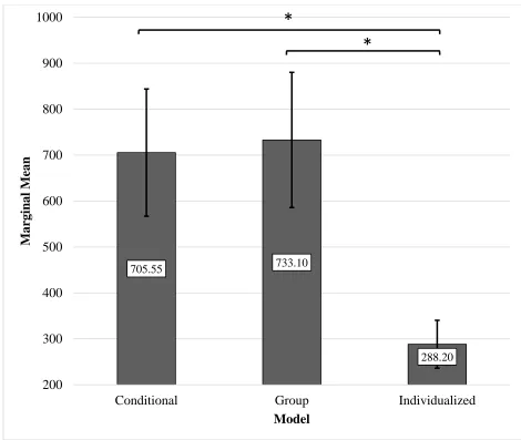
Figure 3: Marginal Means of G2 Values for the Three Models ... 35
Figure 4: Marginal Means of 2
viii
List of Appendices
Appendix A: Formulae for the Probabilities of Engaging Decisional Control structure
element i, Pr(ti) ... 54
Appendix B: All Group Canonical Correlations ... 56
Appendix C: All Group Correlation Matrix for Psychometric Measures and Fit Indices ... 57
Appendix D: All Group Correlation Matrix for Psychometric Measures and Fit Indices (continued) ... 58
Appendix E: Probability Rating Sheet ... 59
Appendix F Letter of Information ... 61
Appendix G: SONA Outline ... 67
Appendix H: Debriefing Sheet ... 69
Appendix I: Ethics Approval ... 72
Appendix J: Hierarchal Structures Presented During Testing ... 73
Chapter 1: Decisional Control: A Normative Model of Coping with Stress
1.1Introduction
Coping with stress is a universal experience and one which requires a complex
interplay of cognitive functions. Coping with stress can be done in a variety of ways, but
choice is key in determining how an individual will respond (Averill, 1973; Thompson,
1981). Through behavioural, cognitive and decisional means, choice in stressful
situations offers an advantage of accessing less-threatening alternatives and greater
control of reducing stress reactions (Averill, 1973). Dissecting how individuals judge
alternatives, when faced with a host of aversive events of varying degrees of
undesirability or harm, and exert personal control to minimize the anticipated stress can
increase our understanding of the cognitive underpinnings of stress. To understand the
role of coping and stress reduction, arguably we must first discuss how a decision maker
(DM) formulates a choice (Thompson, 1981).
Beginning with a discussion of normative decision theory, accepted theories and
their relevance to our model will be introduced. Particularly, the distinction between
normative and descriptive models in decision research will be elucidated. Following this,
a normative model of Decisional Control (DC) will be presented in detail along with its
underlying game-theoretic architecture. Finally, planned model testing and fit will be
discussed as it pertains to necessity testing. When speaking of necessity testing, a
distinction from sufficiency testing is needed. The primary goal of the present study is to
explore sources of differential conformity between our collected data and the theoretical
predictions posited by our formal normative model. While a secondary aim of this
research is to understand how psychometric correlates may relate to the operation of the
model, the primary interest lies in examining sources of improved fit (necessity testing).
Such sources include the historical distinction between objective and subjective
properties of stressor processes at an individual and group level (Heukelom, 2008;
Rappaport, 1983). Specifically, I examine if there is conformity or departure from
objective utilities imposed by the environment and whether improved model fit is
observed when taking into account the representation of the environment by the
individual (subjective utilities; elaborated on below). Lastly, the aim is not to see whether
sufficiently or to improve model fit, but to examine tendered sources of improved
empirical fit to predictions.
1.2Normative Decision Theory
Beginning in the 1950s, cognitive psychologists began focusing on two questions:
how do people make decisions and how should decisions be made (Edwards & Fasolo,
2001). While related, the two questions frame decision-making in two separate ways. The
first is concerned with what choice is made (the final result of a decision), while the latter
incorporates notions about a DM’s use of cognitive mechanisms in explaining how the
decision is reached.
The second question is also concerned with the final result, but in this instance the
process involved in making the decision becomes the focus. A driving force behind this
area of research stemmed from a pursuit to improve decision-making ability through
understanding how individuals judge between alternatives (Edwards & Fasolo, 2001). In
order to separate the two concepts, the terms normative and descriptive were applied to
decision-making theories.
In a descriptive theory, the source of interest is how people make decisions. These
theories are descriptive of the process (from presentation of a dilemma to the choice
made). Theories concerned with how a decision should be made are referred to as
normative. The emphasis of normative theories rests on understanding or explaining how
a DM incorporates environmental demands and intellectual tools available to help make
the best possible decision. The idea that a best option exists and that it should be the goal
of a decision is prescribed by a normative approach. In short, a normative model could be
viewed as one with a hypothesized arsenal of cognitive tools used to estimate and
incorporate environmental demands in the process of making a decision. On the other
hand, a descriptive model expresses how the underlying arsenal is actually appropriated
to lead to a decision. It does not attempt to explain which components of the arsenal exist
or how they function together to lead to the decision made.
To identify and quantify the “best” choice under a normative theory, cognitive
psychologists interested in decision-making rely on mathematics and three specific rules
which encompass normative decision theory (Edwards & Fasolo, 2001). The three rules
(hereafter referred to as Bayes), and maximization of expected utility (Max EU). Each
rule will be discussed in turn to an extent that is relevant for understanding its role in the
present research.
1.2.1Multi-attribute utility (MAU).
In order for an individual to make a decision there must be a choice between two
or more options. Generating the list of available options can be cognitively taxing as the
number of options available to the DM grows. Sometimes the list of options is exhaustive
and fully specifies directly what outcomes occur when selected (e.g., in a quantitative
closed form solution). An example of this could be choosing what to eat at a restaurant.
When you order something off the menu, that selection will be what you receive.
Commonly, what occurs instead is that events beyond the DM’s control combine with the
options available to determine what outcome occurs. An example of this second case
could be choosing which route to take home from work and its impact on your trip time.
You might choose to take the highway instead of a variety of side-streets, find it
unfortunately deadlocked (an event beyond your control), resulting in a very long and
unexpected commute.
In normative decision theory, the options available are called “acts” and the
events beyond the DM’s control are referred to as “states” of the environment. An
important element of states is that they are considered mutually exclusive and exhaustive
of one another; states and state selection have no effect or relation to other non-selected
states. In order for a DM to make a choice, the outcomes comprised of acts and states
require some sort of comparable value relative to one another. To be measurable and
comparable, they must all share the same measurement scale. However, all assessments
of value are entirely subjective of the DM and can vary from one individual to the next.
In this respect, all outcomes are considered subjectively different and are referred to as
“utilities” in normative decision theory. MAU is the process of aggregating utilities to
create an overall subjective score for choice comparison.
However, subjective utilities are not always the only type of utility present.
Sometimes there can be objective utilities; utilities which possess the true ranks of
outcomes. For example, someone might subjectively appraise their choice of braking at a
intersection. Objectively this may be false if statistics quantitatively illustrate that it is
three times more likely that an accident will occur if they choose to brake. Problems can
arise in real world scenarios like this and have consequences for the DM. In this case, a
normative model would subscribe to the best objective utility to choose (going through
the yellow light), but a descriptive model might find that selection is made using a
subjective utility evaluated highest by the DM (braking at the yellow light). To
investigate which conditions are operant under the normative model, subjective and
objective utilities must be considered and compared (Heukelom, 2008; Rappaport, 1983).
More on this topic will follow in subsequent sections on model testing and fit.
1.2.2Bayes’ theorem of probability theory.
In addition to subjectively evaluating utilities, most decisions have a degree of
uncertainty to them. Decisions may lead to one or more outcomes beyond the DM’s
control. However, DMs often have varying degrees of information about the possibility
of one outcome or the other. This information permits judging of the probabilities of the
outcomes related to that choice, such as in instances where Bayes’ theorem can be implemented. Bayes’ theorem assists in choice selection by incorporating prior evidence
to help in assessing the probability of a particular outcome (Bayes & Price, 1763). DMs
use this process known as “fallible inference” or “inference under uncertainty” (Edwards
& Fasolo, 2001) to make judgements regarding which outcomes are likely to occur for
any given act under a particular state. Using our above traffic example, if the DM had
been rear-ended multiple times when choosing to brake at a yellow light, they may have
updated their belief to now believe that going through the intersection is best. The prior
information that they bring into the decision influences their beliefs and, in this case, their
subjective utility aligns with the objective utility. However, if the DM had never been
rear-ended braking at an intersection and had done so hundreds of times, they may hold
an incorrect belief that their subjective utility is the best choice. Even when additional
information is introduced, such as explaining that statistics show it is less optimal to
break at the light, it is possible the DM may hold their subjective utility higher still.
Further exploration of this and similar concepts is beyond the scope of this present
Relevant to this study is the notion that judging between utilities does rely on prior
learned, experienced, or provided knowledge.
1.2.3Maximization of expected utility (Max EU).
Combining aggregates of relevant utilities and probabilities leads us to a
quantitative basis upon which acts can be ranked by DMs. As both utilities and
probabilities are subjectively determined by DMs, normative decision theory refers to the
aggregates of both as “subjectively expected utilities” (SEUs). Max EU is the process of
maximizing the desired outcome by selecting the act with the largest SEU value.
Specifically, the last rule dictates choosing the act with the highest utility when outcomes
contain no uncertainty and choosing the act with the highest SEU when uncertainty is
present (Edwards and Fasolo, 2001).
While this normative theory is a large oversimplification for generating a
decision, as undoubtedly a number of cognitive processes are present in each step of the
process, it acts as a good referent for the present work. A very thorough review of the
literature can be found in Edwards, Miles, and Von Winterfeldt (2007) and Von
Winterfeldt and Edwards (1986). It should be evident, however, that through the
exploration of these three rules, the process by which individual DMs come to make a
decision is largely subjective and can require the use of a variety of cognitive processes.
Particular individuals may favor careful selection of acts, desiring a large amount of
information prior to choosing one, while others may be more resigned to have a selection
delegated to them. Two decision-making strategies related to these sorts of differing
approaches are maximization and satisficing. In maximization, a DM exhaustively
considers all acts in order to find the one with the best utility, whereas a DM adopting a
satisficing strategy will evaluate acts until they find one that is suitable (Simon, 1956).
Choosing a satisficing strategy does not disqualify the possibility that the DM was able to
apply the three rules of normal decision theory, but decided the effort was not justified to
exhaustively search for the objectively best utility. Nor does choosing a maximizing
strategy assume that the DM will choose the objectively best utility, as their subjective
utilities or their application of the three rules may be flawed. Clearly decision-making is
an individualized process likely informed by a variety of dispositional factors. So too is
1.3Decisional Control
DC is a method of coping with stress in which the DM positions oneself in a
stressor situation so as to avoid situational components harboring higher probabilities of
threat (Lees & Neufeld, 1999, p. 185). The underlying assumption is that a DM, when
faced with a selection of varying levels of subjectively adverse events (acts), will make
probabilistic judgements (arguably a cognitively-intensive process) about the threat
inherent in each situation (states). The DM then makes a choice to pursue the act they
believe has the lowest level of stress associated and best chance for a favorable outcome.
Notably, this normative model is well positioned in normative decisional theory and
follows the three rules discussed earlier.
As normative models make use of mathematics to discern MAX EU, it is
facilitative to start with a practical example that explores the environmental framework
and begin introducing some of the equations used in the DC model.
1.4Environmental Framework of Decisional Control
Stress can range in severity (from benign to behaviorally and/or cognitively
paralyzing) and can be evoked by a number of different scenarios (from adverse social
events to situations with a chance for severe discomfort or physical harm). Many real-life
scenarios can be drawn on to construct elements in a game-theoretic infrastructure
composed of stressful alternatives. According to Rasmusen (2007), a game-theoretic
infrastructure is one in which the following four elements must be present: a player (or
players), information and actions available at each decision point, and the payoff for each
outcome. Routed in game theory (Von Neumann & Morgenstem, 2004), well-defined
mathematical objects are structured in nested hierarchies (decision trees) with each node
representing a choice the player (DM) can make, each branch attached to a node
representing an action, and each leaf following an action representing a payoff
(Fudenberg & Tirole, 1991). As will be illustrated in the example to follow, a
game-theoretic infrastructure can be constructed to model and test our normative model of DC.
For a real-world example, imagine that you have been invited to two separate social
gatherings on the same day in similar venues. Each has the same number of guests, but
varies in the people attending. At both gatherings, there are people with whom you are
may prove stressful, but you have decided to at least talk to the person seated beside you
at your assigned table. For simplicity’s sake, we will assume there are four people at each
gathering (each one at a separate table) with whom you are particularly averse to having
to interact with. You predict the conversation will probably lead to adverse social
interaction (e.g., a strong differing of opinions). These eight individuals could be ranked
ordered from 1 to 8 (t1, t2, …, t8; t representing threat of an adverse stress-inducing event;
an act). There is a discernably increasing probability that a conversation will result in an
adverse social event (t8 being the highest probability, and t1 being the lowest).
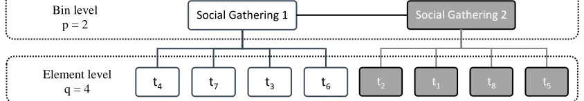
This example takes the form of a nesting-nested hierarchy in which the DM
potentially engages one discrete (mutually exclusive) entity within a tier. The social
gathering and the adverse interactions make up the architecture of our two-tier design
(with parameters p and q; where p = the number of social gatherings = 2 and q = the
number of eligible interactants within each = 4). This architecture is substantiated in
Figure 1.
As in life, control over which entity (node) is engaged is not always within the
DM’s control. DC can sometimes only be applied at certain tiers or not at all. In this
model C is usedto represent the scenario structure in which the DM has an unfettered Element level
q = 4 Bin level
p = 2 Social Gathering 1
t4 t7 t3 t6
Social Gathering 2
t2 t1 t8 t5
Figure 1.An example of a nesting-nested hierarchy (decision tree) with ti
elements randomized at the most subordinate level. Nodes are located along
horizontal lines, with two at the bin level and four within each bin (eight total). In this
example, ti elements are illustrated as static, but would be randomly ordered each
time the hierarchy is displayed. The two bin groups have been coloured differently
choice (they have predictive information and decision-making power); N to represent
external assignment with information but no decision-making power; and U to represent
external assignment in which the DM has no information or decision-making power. To
capture the essence of conditions U and N, their assignment is random from available
options. In this way the elements are neither predictable or controllable for U or
controllable for N.
Considering this two-tiered example (Figure 1), DC can succinctly be expressed
in sentential logic. The definition of DC for a two-tiered hierarchy is
∃J = {x1, x2} ∋∀ xi∈J, xi = C⊻ (U⊻N), (1)
where x1,2 denote the DC conditions for the upper and lower tiers, respectively (Neufeld,
Shanahan, & Nguyen, 2014; Shanahan, Nguyen & Neufeld, manuscript in revision). Put
simply, at each level of the two-tiered hierarchy, either a C, U, or N can be a presenting
condition to be engaged by the DM. The total number of combinations form a set of J; in
our example there are nine pairs, as ordered on the first and second tier (CC, CN, CU,
NC, NN, NU, UC, UN, and UU). Any individual combination is further referred to as j in
the set of J. Keeping with our example, in an instance of CU, the DM would be able to
choose which party to attend but have no information about who is attending (the ti’s
nested within each party) nor any choice of which of the four people they will be required
to sit beside. Alternatively, in NC, the DM will know which party they are attending
(perhaps they were forced into attending one gathering by that gathering’s hostess;
information but no control in the gathering selection). In this scenario, however, they are
told by the host the table at which each of the four people attending will be sat and the
DM is given the choice of the table at which they would like to sit (information about
which 4 individuals are attending and party-wise control).
In addition, each of the pq elements of the two-tiered hierarchy, has an unique
appraised probability of adverse-event occurrence ti (Shanahan & Neufeld, 2010) of
{t1<t2< …<ti< …tpq}; tj<ti iff j<i ; ti∈ [0,1]. (2)
As denoted in Equation 2, the threatened event is a Bernoulli outcome (either it
happened/was encountered, 1, or not, 0) and t is the probability of its occurrence. In
essence, and as stated in Equation 2, there are a number of possible levels of threat (i.e. t1
discernibly worse. As these discrete amounts are mutually exclusive and exhaustive, only
one level of threat (e.g., a gauche interchange is the occurring outcome; ti is the
probability of its occurrence) will transpire and the probability of it occurring Pr(ti) is
related to the level of expected threat, E(t), expressed as
= E(t)
(3)
Each of these ti values is randomly dispersed over the pq elements and can be engaged
with different probabilities based on the conditions of control available to the DM.
Assuming that stressor-event magnitude is such that those with higher ti values are
avoided to a greater extent (thus yielding lower probabilities), we can assume that when
choice is given to the DM they will select options in favor of achieving the smallest ti
value available (referred to before as a maximizing or maximax strategy; Janis & Mann,
1977; Morrison, Neufeld, & Lefebvre, 1988; Rappaport, 1983). Given CC, it is assumed
that the DM will always select t1 upon making the appropriate number of cognitive
appraisals required to discern the decisions necessary in reaching it. In our example, this
requires only two operations of DC – to select the social gathering (bin) that contains t1
and then select to sit at the table (element) with the individual representing t1.
Using basic combinatorics, a potentially helpful way of visualizing the above
engagement and probabilities is through a visual example using bin or urn terminology.
Imagine transparent bins labelled t1 through t8, each containing an equal number of balls,
some black and some white. The black balls represent an adverse event and the white
balls represent a null event (a non-stressful event). If we say there are 8 balls in each bin,
then the t1 bin might have 1 black ball and 7 white balls and the t8 bin might have 7 black
balls and 1 white ball. These balls represent a Bernoulli outcome (there are only two
possibilities), but the probabilities of drawing either a white ball or a black ball vary
based on the bin. Further, the probability of accessing different bins varies based on the
conditions of control (the choice-scenario architecture). The DM will attempt to always
reach the t1 bin (if available), as the probability that they will draw a black ball (encounter
an adverse event) is minimal. In this way, the probability of drawing a black ball is nested
pq
within the probability of engaging a particular bin. If we relate this back to our example
depicted in Figure 1: if you happen to find yourself in a CU condition, a
maximizing/maximax strategy would dictate you would choose to engage in social
gathering 2 in hopes of being assigned to table 1 (where the person represented by t1 is
present). If you happen to be assigned to table 5 (t5) instead due to the uncertainty (U) at
this level, it is still possible that your interchange with the person who you do not like at
that table will not result in an unpleasant experience (i.e., experience a null event;
although probabilistically you are more likely to experience an adverse event).
In scenarios where p and q are larger than in the above example (i.e. when there are more
nested hierarchies, more elements within each, and a mixture of decisional-control
conditions), there is a greater information processing demand on the DM (Shanahan,
Pawluk, Hong, & Neufeld, 2012). This can be a source of stress in and of itself; one
which must be balanced with the stress of the adverse events. This relationship is
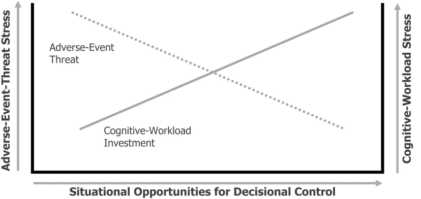
graphically represented in Figure 2.
As cognitive processing (and associated stress) increases, with increased potential
outcome-set size, so does the probability of engaging the lowest-tier element (ti).
Alternatively, as cognitive processing is reduced (with the inclusion of more N
Situational Opportunities for Decisional Control
Adverse
-Eve
nt
-Th
reat S
tr
ess
Cogn
iti
ve
-Workload
Stress
Cognitive-Workload Investment
Adverse-Event Threat
Figure 2. A simplified graphical representation of the hypothetical relationship between
conditions), the stress related to cognition decreases but the probability of engaging in a
higher-tier element increases. This reciprocal relationship between predictive judgement
investment (cognitive workload or “challenge”) stress and exogenous-event threat stress
is what is known in decisional science as an “incompatibility of criteria” (Tversky,
1972a; Tversky, 1972b). Individual differences in coping strategies may be influenced by
this dynamic interplay of sources of stress. Some individuals may prefer to adopt a
maximizing/maximax strategy in order to make the “best decisions” in their pursuit of
minimal ti, whereas other’s may be willing to tolerate ti values below t5 (for example) if it
requires less cognitive workload (weighing choices; an example of adopting a satisficing
strategy). Different susceptibilities to one form of stress or the other, as they interface
with prevailing DC conditions, represent person-environment fit examined here.
In defining a situation amenable to our above example, certain notation is used to
specify the combination of p and q parameters (the number of elements at the first and
second tiers of the DC architecture) and the pair of choice conditions from among C, U,
and N that were present (one at each tier). Typically, the encounter is denoted “ZDC
combination; pq”, so in the example of CU we would report that this encounter took the form of ZCU; 2,4. Let us revisit the NC example, but this time combine it with Figure 1. If we
assume that the DM was forced into attending social gathering 1 by that event’s host
(condition N, meaning an assigned element from the p elements composing the top tier,
the assignment being disclosed at the outset). Next, they are made aware of the location
of the four guests attending that could result in adverse social exchanges (and associated
stress) and are able to choose which one to sit beside (C, meaning choice applied to the q
elements of the lower tier). From Figure 1, we see that the DM can only choose from t3,
t4, t6, and t7. We assume that they will likely choose t3 as it is the act with the lowest
probability for an adverse stressful encounter. If this scenario were run a few times, the
number of times each ti value was engaged would be reported as nti. Since N is randomly
selected each time and there is a p of 2; one would expect that social gathering 1 and 2
would be assigned an equal amount of times. Since t1 is eligible for selection at social
gathering 2, one would predict, that if the scenario of ZNC; 2,4 was run 10 times, that nt1=5
and some combination of tis other than t1 = 5 (as the ti are shuffled each encounter; unlike
(Pr(t1) = 1/p). In fact, all the probabilities for ti can be readily computed for any
two-tiered encounter using the formulas located in Appendix A (Neufeld, 1999; Shanahan,
2016; Shanahan & Neufeld, 2010). Some probabilities require combinatorics, based on
whether t1 is able to be engaged by the DM. Upon further investigation of each, we can
see that certain combinations of conditional control are favorable to others (based on their
probabilities of achieving t1 and expectation of threat E[t], which again entails Pr[ti]ti
from Equation 3). It is important to note that C must be present at one level in the
scenario for DC to be available at all and that U at a subordinate level increases E(t)
significantly more than when it is positioned at the upper level (Shanahan et al., 2012;
Shanahan & Neufeld, 2010). Putting all of these elements together, it should be
self-evident that we have created a game-theoretic paradigm susceptible to testing. Each
participant assumes the role of the DM, they are given differing levels of information and
action at each node, and they are aware of (or learn) the differing payoffs (ti values)
related to each outcome. Unique to this DC normative model is the use of stochastic
outcomes (Osborne & Rubinstein, 1994). By integrating stochastic outcomes, the
environment has an active role in deciding the DM’s fate. This can be observed in
conditions where control is not present, such as when a node is either an N or U
condition. The environment either withholds information and choice or choice alone and
assigns the DM a random action. We have a normative framework (the architecture)
upon which we can test if participants conform to our predictions.
1.5Mixture Modelling
By fitting choices to a quantitative framework, we can disentangle the interplay of
different cognitive processes involved when judging environmental stressors. Through
the individual differences people display in similarly defined situations, we create a
normative model representing person-environment fit. Captured quantitatively, these
differences can illustrate differential dispositions towards engaging in presented
opportunities for choice (a descriptive model), which we can test against our normative
model of predicted probabilities (afforded by our closed-form equational system). As
coping strategies (and their underlying cognitive processes) are largely unique,
individuals will vary in their task performance in situations amenable to DC. At the same
model of DC performs with respect to a consensual, group-extracted, cognitive mapping.
As such, three separate models are required; a normative model (based on conditions
inherent in the environment), an individualized model (based on subjective appraisals of
the environment), and a group model (based on the averaged subjective appraisals across
the group).
One of the first requirements in setting up a mixture model is defining parameters.
Parameter estimation normally requires random sampling from a particular conjugate (i.e.
mathematically tractable) prior distribution that models the probability distribution of the
parameters (i.e. rate or probability) we are looking for. One advantage of our particular
setup is that we do not have to do this. We have our own discrete probabilities generated
from the ground up by our DC architecture. The base-distribution parameters which
pertain to the decision process itself are defined (ti values) and are subject to a probability
mixture, whose finite discrete probability mixing parameters are Pr(ti). We have already
discussed the hyper-parameters above which help define the base-distribution; they are C,
U, N and p and q. As we have already set up all of the architectures, including forming all
our combinations (j) in our set (J) and their resultant probabilities (probability of base
distribution parameter, Pr(ti)). As such, we already have what we need to form
multinomial likelihood functions involved in model testing. We are at an advantage
having created a closed form solution, as we are able to generate every single discrete
value. This can be likened to “samples” and “populations” in classical statistics.
Typically, one samples from a population to generate a representative group upon which
generalizations can be formed. In our case, we have the population of explicitly defined
values and do not need to sample. In order to validate the model using quantitative
predictions, engagements of particular ti and their related stochastically distributed ti,
whose Pr(ti) values are governed by the prevailing structure (j), are used to create
multinomial likelihoods.
1.6Model Testing and Fit
The multinomial likelihood (ML) of nti (the number of times each ti value was
engaged) is defined similarly to how an encounter (ZDC combination; pq) was defined; ML DC
(4)
In Equation 4, ZC,U,N; pq is the total number of times a particular encounter was
experienced, i.e. Nti is the number of ti engagements within that encounter, and Pr(ti) is
the model stipulated probability of engaging a particular tiwithin that encounter. Further,
the prior probabilities of each of j combinations, πj, within the J set of decisional
structures can be represented by the combined multinomial likelihood (Shanahan et al.,
manuscript in revision)
(5)
For the two-tiered DC structures, there are 9 unique combinations (j) possible within the
set of J. These unique structures are made of C, U, and N at the bin level, factorially
combined with C, U and N at the bin-element level (the J structure-combinations of j are
mutually exclusive and exhaustive; the πj sum to 1). Upon calculating a combined
multinomial likelihood for each participant, we will have the necessary values of the
descriptive model upon which to compare the theoretical predictions of our normative
model. In short, we will compare our generated normative predictions to the descriptive,
observed participant responding and determine how different element engagements (ti)
selectively conform to predictions from the prevailing j combinations (Shanahan et al.,
manuscript in revision). If we consider the prior case and apply our static CU example,
we would expect our participants to always select social gathering 2 (in attempt to
achieve t1). Due to the U nature of q, we would expect t1, t2, t5, and t8 to be engaged an
equal number of times (1/q = 1/4).
When we speak about model fit in the present case, we are referring to how well
the normative model-generated expected frequencies correspond to the actual observed
frequencies of participants (the descriptive model). Here, we would want to see if
possible within our Figure 1 example, would show an almost identical pattern of nti as we
would predict from our model assumptions. This equivalence is tested using the
likelihood ratio chi-square statistic G2. As no parameter estimates were necessary (due to
our architecture, as mentioned above), both Akaike and Bayesian Information Criteria
(which are both used to adjust G2 based on the number of parameters being estimated) are
not applied. As such, G2 is simply equal to -2 ln multiplied by the likelihood ratio.
To estimate fit of the different descriptive models (Group model and
Individualized model), we take the participant generated data and test its fit with our
DC-tendered model’s fit (Shanahan et al., 2012). To compute G2, a generic saturated model is
required to form the denominator of a likelihood ratio. In the latter case, the DC
predictions are replaced with observed engagements; instead of the probability of ti, the
actual number of ti engagements out of the total number of encounters are used. The
generic descriptive model is used as a normalizing factor to create a G2 value. This is
illustrated as
G2 = - 2 ln (Likelihood Function Likelihood Function DC model
generic saturated model)
= - 2 ln (Likelihood Ratio) (6)
≈ χ2, when n is large.
In contrast to our DC model used in the numerator, the generic, saturated model used in
the denominator replaces model predictions with observed proportions of ti selections
(Riefer & Batchelder, 1988). Additionally, to compliment the G2 value, a Pearson χ2
value (Cohen, 1988, Chapter 7) will also be computed as the two converge with a large
number of observations.
Based on results from a small simulation, the model of DC does perform as well
as the generic saturated model (Shanahan et al., manuscript in revision). If our predictions
and observations are close, we would expect a very good (low) G2 and Pearson χ2 value
for our tendered models, indicating their ability to accurately predict empirical
probabilities of responding. This serves as an estimate of model fit, whose sources of
change and whose psychometric correlates are the subject of the current thesis.
In order to quantify and empirically test this environmental framework of DC and
explore individual differences in responding, behavioral (e.g., choice selection and their
measures (e.g., verbal reports, numerical ratings) of stress are collected. Past research has
supported the use of these empirical measures quantifying DC composition (Shanahan &
Neufeld, 2010). Gathered empirically, the complex interplay of the above indicators of
stress can be disentangled to reveal differential dispositions in situational engagement
and should conform to predictions of fluctuating levels of stress created by the
environmental framework at both the group and individual level. However, the focus of
the present thesis squarely is on sources of model fit. Other collected responses, including
psychophysiological data, response times, and indices of stress generation will be
analyzed in the future.
Psychometric measures selected to explore individual differences in sources of
model fit include the Desirability of Control (DOC; Burger & Cooper, 1979), Need for
Cognition (NFC; Cacioppo, Petty, & Kao 1982), Intolerance of Uncertainty (IOC;
Freeston, Rheaume, Letart, Dugas, & Ladouceur, 1994) Uncertainty Tolerance Scale
(UTS; Dalbert, 1996), the General Decision-Making Style questionnaire (GDMS; Scott &
Bruce, 1995) and the Endler Multidimensional Anxiety Scale’s Trait scale (EMAS-T;
Endler, Parker, Bagby, & Cox, 1991). Selection of measures was informed by previous
DC research or exploratory in nature. Elaboration of the measures is provided within the
methods section.
1.7Aim of Current Research
Thus, one aim of the present study is to implement a game-theoretic infrastructure
upon which a probability mixture model can be built and tested using a normal
population (undergraduate students). This infrastructure/environmental framework will
allow the development of precise likelihoods of stress-relevant events and the ability to
test the model at both an individual and group level (Shanahan et al., manuscript in
revision). By implementing a self-contained model of DC, we can not only determine the
probabilities of how individuals within a DC amenable scenario should respond
(objective utility), but also use those computations to test our model (a combination of
top-down and bottom up approaches to validation). Candidate sources of departure from
the normative model (contingent/conditional-probability-based) predictions, notably
departures in the form of individual and group cognitive mapping of ti (subjective
model prescribed values (objective utilities and maximizing/maximax selection strategy)
and be correlated with psychometrics. This correlation encompasses the second aim of
the present research. Doing so will allow for estimation of ti values, to which the
maximizing/maximax-strategy component of the normative model potentially applies,
and also residual departure subsequent to allowing for individualized ti estimation.
In summary, the intended purposes of this study are two-fold: a) to test the normative
game-theoretic probability mixture model created for DC and b) to investigate sources of
departure from the normative model including through the use of psychometrically
profiling individual differences in DC “aptitude” (amenability).
The resultant model-based findings will provide empirical evidence that identifies
previously untapped model-testing predictions, including choice-selection behavior and
multinomial likelihood and Pearson χ2 implementation of DC. If the DC normative model
predictions align with empirical observations, the model could be adapted for use in
future studies with clinical populations with known cognitive and decisional difficulties.
This could allow theoretical and empirical exploration and interpretation of group
differences in navigating stressful situations, which could increase our knowledge of
aberrant or dysfunctional cognition leading to suboptimal, cognition dependant coping
strategies in clinical populations.
Chapter 2: Methodology
2.1Participants
Participants were recruited from Western University’s undergraduate Psychology
Research Participation Pool as partial fulfilment of course credit. Fifty-eight participants
were recruited and tested. Twelve participants were removed as a result of a significant
change in the paradigm (n = 8), a computer hard drive failing mid-experiment (n = 2), or
a lack compliance to the task/poor motivation (n = 2). The final participant sample
consisted of 20 males (Age M = 18.2, S.D. = 0.52, Min = 17, Max = 19, Mode = 18, and
Mdn = 18) and 26 females (Age M = 18.7, S.D. = 1.25, Min = 17, Max = 21, Mode = 18,
and Mdn = 18).
2.2Inclusion Criteria
In order to participate in the present study, individuals needed to be under 30
years of age, right-handed, and self-reported good English reading comprehension. Age is
positively correlated with diminished electrodermal activity (Boucsein, 2006), with
noticeable age-related skin changes posited to influence electrodermal activity beginning
at 30 years of age (Boucsein, 2006). The criteria for age was due to this phenomena, as
psychophysiological data was collected for future analysis and not as part of the present
thesis.
2.3Exclusion Criteria
The presence of a self-reported hearing problem is this study’s only exclusion
criteria.
2.4Apparatus
Equipment used for data collection consisted of three separate hardware
platforms, one for cognitive, psychometric, and psychophysiological collection.
2.4.1Cognitive research platform.
Cognitive data collection occurred on an internet-disabled desktop computer with
Windows 7 operating system. The participant and computer were in a room separated
from the experimenter by a one-way mirror. The participant was positioned so the
attention to the task, any discomfort with the adverse noise, choice selections, and time
spent on instructions. A bell located on the participant’s desk was used to signal task
completion or request assistance. Presentation of stimuli and collection of behavioral
responses were completed on the computer using behavioral experiment software
(E-Prime 2.0). Additional responding related to the learning paradigm was collected on
paper forms.
2.4.2Psychometric research platform.
The Measures phase occurred in the data collection area of the research laboratory
using an internet-enabled Gateway laptop running Windows 7. Paper-based
questionnaires were transferred to an online survey software platform (Qualtrics TM), and
this software was used to administer questionnaires electronically.
2.4.3Psychophysiological apparatus.
Psychophysiological data was collected using equipment manufactured by Biopac
(BIOPAC Systems, Inc., Goleta, CA). The MP-150 Data Acquisition System, in
conjunction with ECG-100C (electrocardiography) and EDA-100C (electrodermal
activity) modules, were used to collect heart rate and electrodermal activity. Heart rate
was measured using two adhesive, disposable, snap Ag/AgCl electrodes in a Lead II
configuration, one on the carotid artery above the right collarbone and the second located
medial above the left ankle. This Lead II configuration was incorporated to avoid
impeding responses and to decrease movement artifacts associated with the participants
making selections with their right hand. Electrodermal activity was measured using two
electrodes on the participant’s left hand, one on each on the first phalanges of the index
and middle finger (i.e., fingertips). The software package AcqKnowledge 4.1 was used to
record the signals associated with these electrodes and perform computations. Logitech
stereo desktop speakers were used to generate white noise at a controlled decibel level
(85 dB) for the informed consent sample and during the Learning and Testing phases.
2.5Measures
Published measures exploring a variety of personality and dispositional
platform (Qualtrics TM) and administered to participants using a laptop computer. The
measures selected explore concepts relevant to DC, including desire for control or
cognition, intolerance of uncertainty, decision-making style, and features of trait anxiety.
In addition, following probability learning trials (described below), a probability
rating sheet and a rank ordering sheet were used to measure a participant’s judgement of
the probability and the ordinal ranking that a particular letter would be followed by an
adverse noise respectively. These sheets were administered after each trial in the
Learning phase and at the conclusion of the Testing phase of the overall procedure.
2.5.1Desirability of Control.
The Desirability of Control scale (DOC; Burger & Cooper, 1979) was developed
to assess motivation to control of events in one’s life. It is a 20 item measure that uses a
seven-point Likert scale (1 = The statement does not apply to me at all; 7 = The statement
always applies to me). A factor analysis conducted by Burger and Cooper (1979) found
five factors accounting for 50.4% of DOC variance: General Desire for Control (e.g., “I enjoy having control over my own destiny”); Decisiveness (e.g., “There are many
situations in which I would prefer only one choice rather than having to make a
decision”); Preparation-Prevention Control (e.g., “I like to get a good idea of what a job is all about before I begin”); Avoidance of Dependence (e.g., “I try to avoid situations
where someone else tells me what to do”); and Leadership (e.g., “I would rather someone
else take over the leadership role when I’m involved in a group project”). The DOC scale
demonstrates good reliability and validity, with adequate construct validity and good
test-retest reliability (α =.78 and α =.76) according to McCutcheon (2000) and has been used
in previous DC research (Shanahan, 2016).
2.5.2Need for Cognition.
The Need for Cognition scale (NFC; Cacioppo, Petty, & Kao 1984; Cacioppo &
Petty, 1982) was developed to assess the tendency and enjoyment in using information
processing when presented with activities amenable to its use. The 34-item Likert scale
has nine anchors (-4 = very strong disagreement; 4 = very strong agreement). The NFC
has strong internal consistency (α =.90; Cacioppo et al., 1984) and measures a single
really enjoy a task that involves coming up with new solutions to problems”. The NFC
has been applied successfully in previous DC research to psychometrically profile
participants (Shanahan, 2016) and abdicate an ability-dependant view of DC in favor of a
personality-dependant view (Benn, 2001, 1995).
2.5.3Intolerance of Uncertainty Scale.
The Intolerance of Uncertainty Scale (IUS; Freeston, Rheaume, Letarte, Dugas, &
Ladouceur, 1994) is a 27-item measure initially constructed to evaluate emotional,
cognitive, and behavioral reactions to uncertainties implicit in situations, oneself, and the
future, as well as the resulting implications of uncertainty on the individual. Items such as
“It frustrates me not having all the information I need” and “I must get away from all uncertain situations” are rated using a five-point Likert scale (1 = not at all characteristic
of me; 5= entirely characteristic of me). While the scale is scored using a single summary
score, a recent review of factor analytical studies has noted a variety of underlying factors
measured by the IUS (Birrell, Meares, Wilkinson, & Freeston, 2011). In their review,
Birrell and colleagues (2011) identified two consistent factors tapped by the IUS
including the “desire for predictability and an active engagement in seeking certainty”
(IUSF1) and the “paralysis of cognition and action in the face of uncertainty” (IUSF2).
The IUS has been successfully used in recent DC research (Shanahan, 2016), correlating
significantly with measures related to DC and possessing a Cronbach’s alpha of 0.91.
2.5.4Uncertainty Tolerance Scale.
The Uncertainty Tolerance Scale (UTS; Dalbert, 1996, 1999) measures the
tendency to evaluate uncertain situations as a challenge or as a threat. Responses to the
eight items fall along a 6-point Likert-scale (1 = strongly agree; 6 = strongly disagree.
Sample items include “I like unexpected surprise” and “I like to let things happen”. The
scale has been used successfully in a number of studies by its creator (Dalbert, 1999,
1996a, 1996b; Otto & Dalbert, 2011) and others (Bardi, Guerra, & Ramdeny, 2009; Bude
2.5.5General Decision-Making Style.
The General Decision-Making Style (GDMS; Scott & Bruce, 1995) questionnaire
is a 25-item measure with five scales comprised of five questions each. Each scale refers
to conceptually independent, but not mutually exclusive, decision-making styles. They
are: Rational, Intuitive, Dependant, Spontaneous, and Avoidant (GDMS-R, -I, -D, -S, and
-A respectively). Scott and Bruce (1995) found that their results supported individuals
adopting a combination of decision-making styles when making important decisions and
reported internal consistency values (Cronbach’s alpha) for each style ranging from .68 to
.94. Items are endorsed along a five-point Likert scale ( 1 = strongly disagree; 5=
strongly agree) and include the following sample items: “My decision making requires
careful thought” (Rational), “When making decisions, I rely upon my instincts” (Intuitive), “I rarely make decisions without consulting other people” (Dependent), “I postpone decision making whenever possible” (Avoidant), and “I generally make snap decisions” (Spontaneous). One item reported missing by Appelt, Milch, Handgraaf, and
Weber (2011) from the original publication for the Rational scale was absent in our
conducted research as well. The 24-item GDMS has been used effectively in the past to
psychometrically profile participants (Shanahan, 2016).
2.5.6Endler Multidimensional Anxiety Scale – Trait scale.
The Trait scale of the Endler Multidimensional Anxiety Scale (EMAS-T; Endler,
Parker, Bagby, & Cox, 1991) is used to measure several facets of trait anxiety. It does so
along four situational dimensions: Physical Danger, Social Evaluation, Novel Situations,
and Daily Routine (EMAS-PD, -SE, -NS, and -DR respectively). Each dimension
describes a situation pertinent to what it is measuring and poses 15 identical statements
regarding the responder’s reactions and feelings. These statements are endorsed along an
intensity scale ranging from 1 (Not at all) to 5 (Very much) and sample statements
include “Seek experiences like this” (reverse scored), “Feel upset”, “Perspire”, and “Heart beats faster”. Coefficient alpha reliabilities reported by Endler et al. (1991) for a
Canadian undergraduate population on all subscales of the Trait scale are over .92 for
both men and women. The EMAS-T has been used successfully in past DC research to
psychometrically profile individual dispositions linked to its application (Benn 2001;
2.5.7Probability Rating sheet.
The probability rating sheet was modelled after one used by Lees and Neufeld
(1999) and consisted of a column of ten blank spaces to write a letter and adjacent 100
mm lines. Each 100 mm line was marked with an anchor at 0, 25, 50, 75, and 100
percent. The sheet is used by participants to demark the probability they believe a
particular learned letter will be followed by a stressor.
2.5.8Rank Ordering sheet.
The rank ordering sheet consisted of 10 blank spaces anchored on the left with the
word “lowest” and on the right with “highest”. A randomized ordering of the 10 letters
participants would learn to associate with a stressor adorned at the top. Participants were
instructed to fill in the 10 blank spaces with the letters in an ordering they believed went
from the lowest to highest probability of being followed by a noise (the stressor).
2.6Procedure
The experiment consisted of four separate phases hereafter referred to as the
Measures, Learning, Practice, and Testing phases (elaborated upon below). Learning and
testing phases were modelled after the general procedures outlined in Kukde and Neufeld
(1994) and Morrison et al. (1988). Prospective participants read and discussed a brief
description of the experiment with the experimenter and were exposed to a one-second
burst of 85 dB white noise from the computer speakers prior to obtaining informed
consent. All participants agreed to continue and none withdrew.
2.6.1Measures phase.
During the measures phase, participants completed the digitized measures (i.e. the
DOC, NFC, UTS, EMAS, IUS, and GDMS) using QualtricsTM software on a laptop
computer in the recording area of the laboratory. A research assistant was present to
answer questions and clarify wording for participants. The measures phase took
approximately 30 minutes to complete.
2.6.2Learning phase.
Following the Measures phase, participants were led to the recording area of the
presented with three rounds of learning trials, each followed by a probability judgement
trial. All instructions were presented on the computer screen and participant feedback
during the probability judgement trials was elicited through the use of the probability
rating sheet and ranked order sheet.
Each learning trial consisted of the same 104 presentations of capital, English
alphabetic letters paired with either an "innocuous event" or a "stressor". Each innocuous
event was a one-second computer screen presentation of a green screen (a non-significant
event) and each stressor was a one second burst of 85 dB white noise from the computer
speakers. The stressing properties of the stressor have been ascertained according to
Thurstonian and other scaled subjective and psychophysiological responses in previous
DC research and related studies (Kukde & Neufeld, 1994; Lefave & Neufeld, 1980;
Neufeld & Herzog, 1983; Neufeld & Davidson, 1974). The 104 letter-outcome pairs and
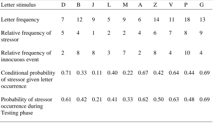
the conditional probabilities of a stressor given a letter are both included in Table 1. For
an example of a conditional probability, the letter D would appear seven times per trial,
two times with a green screen (innocuous event) and five times followed by the white
noise stressor (giving a conditional probability of 5/7=0.71%). Ordering of these
letter-outcome pairs was randomized across participants and between trials; all participants
received the same pairs, but in completely random order. The ten letters selected were
identical to those used in Kukde and Neufeld (1994) and Morrison et al. (1988). Their
selection was such that the probability of misidentifying one letter for another was less
than 0.10, as indicated by Townsend's (1971) confusion matrix. The paradigm used in
this study and the above mentioned studies is one pioneered by Estes (1976). Estes’
paradigm allows differential anticipatory stress to occur in response to the chosen letters
due to memory association mechanisms of probability learning (cf. Estes 1976). Unequal
letter frequencies are such that stressor and innocuous events are uncorrelated (r =.02),
but still amenable to Estes’ (1976) model of “categorical memory”. In essence, Estes’
paradigm is designed such that each letter possesses its own inherent probability of a
stressor and is implicitly separate from the probabilities of other letters. Past research has
evidenced that participants’ judgement rankings have a greater tendency to align with the
frequency of stressor occurrences than the conditional probabilities (Morrison et al.,1988;
probabilities from participants in past studies (Lees & Neufeld, 1999; Morrison et al.,
1988) were averaged with the conditional probability to create a hybridized probability.
This hybridized probability is given in Table 1 as the probability of stressor occurrence
during the Experiment phase. It dictates the probability of feedback during the Testing
phase to better align with participant expectations of stressor/innocuous event probability.
Table 1
Letters for Stimulus Presentation (During Learning and Testing phases) and Associated
Frequencies and Probabilities
Letter stimulus D B J L M A Z V P G
Letter frequency 7 12 9 5 9 6 14 11 18 13
Relative frequency of stressor
5 4 1 2 2 4 6 7 8 9
Relative frequency of innocuous event
2 8 8 3 7 2 8 4 10 4
Conditional probability of stressor given letter occurrence
0.71 0.33 0.11 0.40 0.22 0.67 0.42 0.64 0.44 0.69
Probability of stressor occurrence during Testing phase
0.61 0.42 0.21 0.41 0.33 0.62 0.50 0.63 0.48 0.69
During each learning trial, a letter appeared on the computer screen for two
seconds followed by a two-second delay and then a one-second innocuous or stressor
event. A three-second inter-trial interval would precede the subsequent letter presentation
to allow psychophysiological responding to return to baseline. Participants were
instructed to say aloud any letter paired with a stressor by saying the letter and the word
"noise". For example, if the letter Z was presented and followed by the stressor, a
participant would say "Z noise". If a letter was not followed by a stressor, they were
letter-outcome pairs from a modified Estes’ (1976) paradigm found to produce the
greatest salience to noise frequency by Neufeld and Herzog (1983) and to enhance traces
in categorical memory on which probability judgements were found to be determined
(Estes, 1976).
To lessen the cognitive demands of the task on memory and enhance learning,
participants were instructed to arrange ten physical blocks, each with a letter written on it,
in order from least to most likely to be followed by a stressor during inter-trial intervals.
Participants were requested to continue to order the blocks within and across all three
learning trials. Participants were informed that all learning trials contained the same
frequency of letter-outcome pairs with only the ordering randomized.
Participants completed a probability judgement trial following each learning trial.
During a judgement trial, participants were presented with a random letter on screen for
two seconds and given a six-second window to record on the Probability Rating sheet the
letter presented and demark on the line the probability of the letter being followed by the
stressor. Judgements were requested under a short timeframe of six seconds to encourage
participants to report their initial beliefs and not deliberate their answers. Participants
then completed a ranked ordering of the letters from least to most likely to be followed by
a stressor on the Rank Ordering sheet. Once all answers were recorded, participants were
given a two-minute break before the subsequent learning trial began. The Learning phase
took approximately 45 minutes to complete.
2.6.3Practice phase.
Following the Learning phase, participants were instructed on the rules of a DC
framework and practiced making selections as they would in the Experimental phase.
Participants were given a sheet containing a separate set of ten letters and their
hypothetical probability of being followed by a stressor. They were instructed to make
selections using these letters for the preliminary Practice phase and informed that the ten
letters they had previously learned to associate with stressor occurrences would be
present in the Testing phase. No stressor occurrences were provided during the Practice
phase trials and feedback was displayed for both correct and incorrect selections to
enhance rule learning. Electrodes and leads were connected at the beginning of this phase