Confidence Interval Estimation of Cumulative Incidence for Clustered Competing Risks

(1)

Western University Western University

Scholarship@Western

Electronic Thesis and Dissertation Repository

2-17-2017 12:00 AM

Confidence Interval Estimation of Cumulative Incidence for

Clustered Competing Risks

Atul Sivaswamy

The University of Western Ontario

Supervisor Neil Klar

The University of Western Ontario Joint Supervisor Merrick Zwarenstien

The University of Western Ontario

Graduate Program in Epidemiology and Biostatistics

A thesis submitted in partial fulfillment of the requirements for the degree in Master of Science © Atul Sivaswamy 2017

Follow this and additional works at: https://ir.lib.uwo.ca/etd Part of the Biostatistics Commons

Recommended Citation Recommended Citation

Sivaswamy, Atul, "Confidence Interval Estimation of Cumulative Incidence for Clustered Competing Risks" (2017). Electronic Thesis and Dissertation Repository. 4441.

https://ir.lib.uwo.ca/etd/4441

This Dissertation/Thesis is brought to you for free and open access by Scholarship@Western. It has been accepted for inclusion in Electronic Thesis and Dissertation Repository by an authorized administrator of

(2)

Abstract

In a cluster randomized trial studying a primary outcome patients are sometimes exposed to

competing events. These are risks that alter the probability of the primary outcome occurring.

Traditional methods of estimating the cumulative incidence for an outcome and its associated

confidence interval under competing risks do not account for the effect of clustering. This may

cause incorrect estimation of confidence intervals because outcomes among patients from the

same center are correlated. This thesis compared six nonparametric methods of confidence

interval construction for cumulative incidence, four of which account for clustering effect,

under competing risks via simulation study. Over the range of examined scenarios, if the

clustering effect is mild (i.e. ICC=0.01), estimators not accounting for clustering never have

significantly worse coverage than those that do. However, in cases with a large clustering

effect (i.e. ICC= 0.05), using confidence interval estimators accounting for clustering should

be considered.

Keywords: Competing Risks; Clustering; Cumulative Incidence Function.

(3)

Acknowledgments

First, I thank Dr. Klar and Dr. Zwarenstein for their guidance and support. In particular,

I would like to thank Dr. Klar for his careful assistance and insight during the preparation of

this thesis.

I thank the Eastern Cooperative Oncology Group for providing with me their data.

Thanks to the faculty, staff, and students in the Department of Epidemiology and

Bio-statistics, who helped me throughout the completion of my degree. I thank my friends in the

Department of Statistical and Actuarial Sciences. I thank the family of Allan Wilson for their

friendship.

Finally, I thank my parents.

(4)

List of Figures

5.1 Number of Patients per Center in EBMT Dataset . . . 56 5.2 Cumulative Incidence of Graft Versus Host Disease Accounting for Competing

Events due to Death or Relapse and associated 95% log-log Counting Process Confidence Intervals at Years 1 to 5 . . . 57 5.3 Number of Patients per Centre in Immediate Arm of ECOG Dataset . . . 59 5.4 Cumulative Incidence of Death due to Prostate Cancer in the Immediate

Treat-ment Arm Accounting for Other Causes of Death and Associated 95% log-log Counting Processes Confidence Interval at Year 10 . . . 61

(7)

List of Tables

2.1 Variance Estimators . . . 19

3.1 Simulation Parameters . . . 23

4.1 Percentage Bias for Variance Estimators Applied to Simulated Data Sample Size=100, ICC=0 . . . 36

4.2 Percentage Bias for Variance Estimators Applied to Simulated Data Sample Size=100, ICC=0.01 . . . 37

4.4 Percentage Bias for Variance Estimators Applied to Simulated Data Sample Size=400, ICC=0 . . . 39

4.7 Coverage of log-log Confidence Intervals Sample Size=100, ICC=0 . . . 42

4.8 Coverage of log-log Confidence Intervals Sample Size=100, ICC=0.01 . . . 43

4.10 Coverage of log-log Confidence Intervals Sample Size=400, ICC=0 . . . 45

4.13 Width of log-log Confidence Intervals Sample Size=100, ICC=0 . . . 48

4.14 Width of log-log Confidence Intervals Sample Size=100, ICC=0.01 . . . 49

4.16 Width of log-log Confidence Intervals Sample Size=400, ICC=0 . . . 51

5.1 Comparison of 95% log-log Confidence Interval Methods for Cumulative Inci-dence at 1 to 5 Years . . . 58

5.2 Comparison 95% log-log Confidence Interval Methods for Cumulative Inci-dence of Death due to Prostate Cancer at 10 Years . . . 60

(8)

List of Abbreviations

Definition First Used

KM Kaplan-Meier Estimator 2

CI(F) Cumulative Incidence (Function) 2

ICC Intracluster Correlation Coefficient 3

GVHD Graft Versus Host Disease 4

Mult Multinomial Based Variance Estimator 11

CP Counting Processes Based Variance Estimator 11

Lin Linearized Variance Estimator 14

Boot1 One-sample Bootstrap Variance Estimator 16

Boot2 Two-sample Bootstrap Variance Estimator 16

Jack Jackknife Variance Estimator 17

EBMT European Bone Marrow Transplant Group 55

(9)

Chapter 1 Introduction

1.1 The Competing Risks Setting

Competing risks data occur whenever study subjects are at risk of experiencing one of

several mutually exclusive events (Kalbfleisch and Prentice, 2002). This situation contrasts

with the classical setting of survival data where subjects are assumed to experience only one

type of event or where an event is composite (e.g. the event is death due to any cause).

Methodology to analyze competing risks data goes back at least to 1776 when Daniel

Bernoulli estimated the increase in life expectancy due to the elimination of smallpox mortality

(Dietz and Heesterbeek, 2002). A brief summary of clinical and methodological questions that

motivated the development of competing risks theory is provided by Birnbaum (1979). Prior to

Kalbfleisch and Prentice (1980), most competing risks methodology used latent failure models

that required specifying the degree of dependence between the hypothetical failure times of

each competing risk. Such assumptions cannot be checked from the data, which only contains

the failure time and the type of failure. Kalbfleisch and Prentice (1980) argued in favour of

modeling based on directly estimable quantities from observed data alone. In this thesis, all

modeling and estimation will follow this strategy.

In clinical studies with time-to-event data, one of the main interests is estimating the

(10)

Chapter 1. Introduction 2

T occurring by time t (Satagopan, 2004). In the traditional survival setting, when there is only one type of event and patients are followed until they experience it or are censored, an

estimator of P(T ≤ t) can be obtained using the Kaplan-Meier method (Kaplan and Meier, 1958). The Kaplan-Meier method can also be applied in a competing risks setting to determine

the cumulative distribution by treating outcomes other than the risk of interest as censored.

This is not always advisable. Indeed, several articles have been recently published cautioning

against this strategy in the statistical analysis of survival data both in medical (Bakoyannis and

Touloumi 2012, Koller et al. 2010, Wolkewitz 2014) and epidemiological research

(Ander-sen, 2011). The main reason is that use of the traditional methods of survival analysis, such

as the Kaplan-Meier method, for competing risks data, could lead to inconsistent estimators

of the probability of experiencing the event. Such methods consistently estimate cumulative

distribution under the assumption of the independence of the competing risks. This is not al-ways an unreasonable assumption. There may sometimes be valid reasons to assume risks are

independent. For example, when patients who enter a study at different times are

administra-tively censored, we need not assume this alters their probability of experiencing an outcome

of clinical interest. But there are many situations in which such an independence assumption

is unreasonable. Consider for example, a trial interested in an event such as death due to a

cancer occurring mostly in elderly patients. If patients enrolled in the trial die from some other

chronic disease (e.g. stroke), it would be inappropriate to still use the Kaplan-Meier estimator

and treat these deaths as censored, as the censoring is likely informative since both cancer and

stroke incidence increase with age. To treat death from illnesses caused by aging as censoring

would underestimate the probability of experiencing the event of interest (Wolkewitz, 2014).

There are also examples where treating a competing risk as censoring can underestimate the

probability of survival. Moeschberger (1995) points out as an example of this, the competing

risk of patients who drop out of a study and move because they have been experiencing success

with the therapy.

(11)

setting, in the competing risks setting one wishes to estimate the cumulative incidence function

(CIF) of a particular risk. If there arekpossible event types, the cumulative incidence for risk

iis defined asFi(t)=P(T ≤t,R=i), whereT denotes the random variable for the time to the

first event andRis a random variable specifying the event type that occurred ranging from 1 to

k. A nonparametric cumulative incidence estimator which accounts for competing events was proposed by Kalbfleisch and Prentice (1980).

Pocock (2007) observes that in the reporting of results from time-to-event studies, displays

of statistical uncertainty in plots of Kaplan-Meir curves are often absent. This may lead to

the over interpretation of treatment difference. Thus it should be encouraged when reporting

the results of a study where competing risks data are analyzed to have not only an estimate

of the cumulative incidence function, but also a value of the precision of the estimate. For

example, in a study on contraceptive use in developing countries, the competing risks examined

were three possible reasons for stopping contraceptives. It was of interest to estimate the

risk of, and a confidence interval for, each of the reasons of discontinuation one year after

administration of the contraceptive (Choudry, 2002). Methods for estimating the variance of

an estimate of the cumulative incidence (and thus for specifying confidence intervals) have

existed since at least Aalen (1978). However, only relatively recently have simulation studies

been conducted comparing the performance of variance estimators for the cumulative incidence

function (Choudry 2002, Braun and Yuan 2007, Iljon 2013). Iljon (2013) states that previous

work has not addressed the question of one-arm estimation because researchers usually focus

on comparing two treatment arms using tests that do not require estimation of cumulative

incidence.

Moreover, the methods developed to estimate the variance of the cumulative incidence

function assume that there is no correlation in the event times of observations, which may not

always be the case. Consider the following scenarios:

1. Antibiotic Treatment for Pneumonia in Stroke patients: Patients from different

(12)

treatment alone. Patients were followed until they are discharged from hospital or

expe-rience the competing risk death (Kalra et al., 2015).

2. Bone Marrow Transplantation for Leukemia: Patients with Leukemia from different

transplantation centres received a bone marrow transplant. Patients were followed until

the development of graft versus host disease (GVHD), the primary outcome, or death

from another cause, the competing event (Zhou et al., 2012).

3. Hormonal Therapy for Prostate Cancer: Patients from different centres are followed

until death from prostate cancer, the primary outcome, or death from another cause, the

competing event (Messing et al., 1999).

In cases where patients come from different centers, as in the examples above, there will

likely be a correlation in response between patients from the same center. This is because

individuals from the same center are more likely to be treated by the same clinician, or be from

the same geographical area, and thus share environmental and lifestyle factors. For binary and

quantitative outcomes, the degree of similarity among responses within a cluster, known as

within-cluster correlation, can be measured by a parameter called the intracluster correlation

coefficient (ICC) (Donner and Klar, 2000). For binary and quantitative outcomes, unbiased

ICC estimators are easily derived using analysis of variance (ANOVA). This may not be true

for time-to-event data however. Kalia (2015) showed ANOVA ICC estimators for time-to-event

data are negatively biased for clustered outcomes.

Clustering effects are also of significant concern in cluster randomized trials when intact

social units (e.g. hospitals, communities), called clusters, are randomized into treatment arms.

The results of this thesis are particularly important for cluster randomized trials with competing

risks endpoints, such as the antibiotic treatment for pneumonia in stroke patients trial described

in Kalra et al. (2015).

Adjustments to competing risks methods have been made to account for clustering in the

(13)

incidence function in a clustered setting has been developed (Chen et al., 2008). But very little

has been written on how to estimate the variance of the cumulative incidence function when

outcomes are clustered, and no study has been performed comparing methods of confidence

interval construction in a clustered competing risks setting. This is despite the extension of

the Consort statement (Campbell et al., 2012) to cluster randomized trials which stresses the

importance of reporting 95% confidence intervals for summary measures of primary outcomes

such as means, risks, and rates.

1.2 Focus of Thesis

We are concerned with confidence interval estimation of a cumulative incidence function

constructed for one sample under clustering. While parametric methods exist to estimate the

cumulative incidence function and confidence intervals, both in the presence and absence of

clustering, parametric estimators require possibly incorrect assumptions about the underlying

survival distribution. Thus the focus of this thesis will be limited to nonparametric methods of

estimation. Confidence interval estimates for a point in time on the cumulative incidence

func-tion will be constructed from a point estimate and variance estimate for the cumulative

inci-dence function. We focus on 95% intervals because these are frequently reported and Campbell

et al. (2012) recommend their reporting.

We will estimateFi(t), the cumulative incidence function for riski, using the nonparametric

estimator described by Kalbfliesh and Prentice (1980). It has the advantage of always being

less than the complement of the Kaplan-Meier estimator (1-KM) (Pintelle, 2006).

1.3 Objectives of Thesis

This thesis has two goals:

1. To compare methods of nonparametric variance estimation and methods of confidence

interval construction based on robust variance estimators for the cumulative incidence

function assuming clustered competing risks data. This comparison is based on a

(14)

estimators will be compared on coverage, percentage missed left and right of the interval,

and interval length. Parameter values for the data generated for the simulation study will

be informed by the example datasets: e.g. number of competing risks, the cluster size

and number of clusters, and the degree of within-cluster correlation.

2. To apply methods of confidence interval construction to the analysis of the Bone Marrow

Transplantation (Zhou et al., 2012) and Hormonal Therapy for Prostate Cancer (Messing

et al., 1999) datasets introduced above.

1.4 Organization of Thesis

This thesis includes six chapters. This first chapter provides the rationale and thesis

ob-jectives introducing the key competing risks challenges for clustered data. Additional context

and background for methods compared in the simulation study is provided in Chapter 2.

Chap-ter 3 outlines the design of the simulation study while the results of the simulation study are

described in Chapter 4. These results are illustrated in Chapter 5 using data from the trials

introduced in Section 1.1. Thesis results are summarized in Chapter 6, where the limitations of

(15)

Chapter 2 Literature Review

2.1 Introduction

This chapter describes in more detail the estimator for the cumulative incidence and

asso-ciated variance estimators to be compared via simulation study in Chapter 4. Including this

introductory section, there are six sections in this chapter. Section 2.2 describes the specific

study design to which the methods will be applied, while Section 2.3 introduces the

mathemat-ical notation used in the thesis. Next, Section 2.4 presents estimators of cumulative incidence

and variance estimators used to construct confidence intervals through the transformations

de-scribed in Section 2.5. Finally, Section 2.6 summarizes the chapter.

2.2 Thesis Setting

The aim of this thesis is to compare methods of confidence interval construction for the

one sample cumulative incidence function using competing risks data from patients treated

at different centers. Only administrative censoring is assumed to occur and between center

differences are assumed to vary at random (i.e. within-center times are positively correlated).

For the remainder of this thesis we will, for clarity of presentation, examine only estimating

the cumulative incidence function of the first risk (i.e. study outcome of interest), and will be

examining scenarios where there is a study outcome and one competing event. The discussion

is generalizable to more than one competing risk and to the cumulative incidence function of

(16)

Chapter 2. Literature Review 8

any event. Moreover, we make no assumptions about the dependence of the competing risks or

degree of correlation between responses from the same cluster. That is, our focus is limited to

nonparametric estimation of variance. We will exclude ANOVA estimators of variance which

attempt to estimate intracluster correlation as these have been found to be biased for

time-to-event data (Kalia, 2015).

2.3 Notation

Denoting the number of clusters in a studyC, we let the number of subjects in cluster cbe

Nc at study entry, forc∈ {1,...,C}. The total sample size at study entry is denotedN and thus,

N=N1+...+NC.

For i∈ {1,...,Nc}, the time-to-event and censoring variables for the ith subject from cluster c

is denoted: (tci,δci), where tci is the time at which an event is observed or the observation is

censored;δci=1 if the study outcome occurred, δci=2 if the competing event occurred, and

δci=0 if the event was censored.

LetMdenote the number of unique event-times when subjects failed from either cause. All subjects are assumed to enter the study at the same time, prior to random assignment, denoted

t0=0. Lett1<t2< ... <tj< ... <tM be the unique observed times at which (possibly more than

one) failure occurs.

For j∈ {1,...M},c∈ {1,...C}, andi∈ {1,...Nc}, letd1ci(tj)=1 if subjectiof clustercfails at

timetjof the study outcome andd1ci(tj)=0 otherwise;d2ci(tj)=1 if subjectiof clustercfails

at timetjof the competing risk andd2ci(tj)=0 otherwise;nci(tj)=1 if subjectiof clustercis

still at risk at (or immediately before) timetjandnci(tj)=0 otherwise.

Then at timetjthe number of failures from the study outcome isd1j=PC_c₌₁PN_i₌C₁d1ci(tj); the

number of failures from the competing risk is d2j=PC_c₌₁P_iN₌C₁d2ci(tj); the number of failures

of any type at time tj is dj = d1j+d2j; and the number of individuals still at risk is nj =

PC

c=1 PNC

i=1nci(tj).

Also note, the number of observations in the study isN=PC

c=1 PNC

(17)

failures from the competing risk,d2=PM_j₌₁PC_c₌₁P_iN₌C₁d2ci(tj). Note M≤d1+d2≤N.

2.4 Competing Risks Estimators

2.4.1 Estimating the Cumulative Incidence Function

In the absence of competing risks, the cumulative distribution function is defined as P(T ≤

t)=1−S(t), whereS(t) is the survival function. An estimator of the cumulative distribution function is 1-KM, where KM is the Kaplan-Meier survival estimator. We discussed in Chapter

1 that this estimator may be inappropriate in the presence of competing risks.

In a competing risks setting, the cumulative incidence function for the study outcome is

defined asF1(t)=P(T ≤t,R=1), where T is a random variable for the time to the first event andRis a discrete random variable specifying the type of event that occurred. R=1 denotes the event of interest occurred, andR=2 denotes the competing event occurred. Unlike a setting where there are no competing risks, the cumulative incidence function does not converge to 1

ast→ ∞, but instead, F1(∞)=P(R=1).

The cumulative incidence function may be written in terms of the subhazards of the study

outcome and competing risk (denotedλ1(t) andλ2(t) respectively). Fori=1,2, the subhazard for riski, the instantaneous event rate, is defined as:

λi(t)= lim

∆→0

P[t≤T <t+ ∆|T ≥t,R=i]

∆ (2.1)

The overall survival function, that is, the probability of being event free from any cause,

can then be written as:

S(t)=exp

−

Z t 0

λ1(v)+λ2(v)

dv

(2.2)

And the cumulative incidence function of the event of interest is:

F1(t)= Z t

0

(18)

Klein and Andersen (2005) note that the cause specific hazard and the cumulative incidence

function require no assumptions about the dependence structure of the competing risks and that

both can be estimated from the observed data, as opposed to being modeled from unverifiable

assumptions. Because the focus of this thesis is on nonparametric methods of estimation, we

will not discuss the model-based methods of estimating competing risks. For model-based

methods of estimating competing risks see, for example, Chapter 4 of Birnbaum (1979).

As shown in equation (2.3) the cumulative incidence can be written in terms of S(t), the event-free probability of survival, and λ1(t) the subhazard of risk 1, so an estimator for the cumulative incidence is given by an estimator for each function.

The formal derivation of these estimators is based on Aalen (1978) and Aalen and Johnson

(1982). However, Pintelle (2006) and Gooley (1999) both provide heuristic justifications. That

is, the Kaplan-Meier estimator can be used to estimate survival, and d1j/nj can be used to

estimate the hazard of the study outcome at timetj. Substituting these estimators into equation

(2.3) gives the following estimator for the cumulative incidence for the first competing risk:

ˆ

F1(tj)= j

X

p=1

d1p

np

ˆ

S(tp−1) (2.4)

where

ˆ

S(tj)= j

Y

p=1

1−d1p+d2p

np

(2.5)

and we define ˆS(t0)=1.

This estimator is consistent when there is no clustering and it is the nonparametric

maxi-mum likelihood estimator (Pintelle 2006; Section 4.2.2). The estimator is also available in

stan-dard statistical software (the R package “cmprsk”, SAS 9.4 under “PROC phreg”, and STATA

14.0 under “stcompet”). Chen et al. (2008) show that ˆF1(t) remains consistent for clustered event times, using the results of Speikerman and Lin (1998), as the number of clusters grows

large, for a fixed cluster size. Since the three examples motivating this thesis presented in the

introduction all have a large number of clusters relative to cluster size, we should not have

(19)

our purposes. However, it is well known that the Kaplan-Meier estimator is biased under

cen-soring, and thus the estimator shown in equation (2.4) is also biased, but Chen et al. (2008)

showed the bias of this estimator is under<0.02 absolute bias, under wide ranges of clustering

and for cumulative incidence values between 0.1 to 0.5.

2.4.2 Variance Estimators Under Independence

Braun and Yuan (2007) performed a simulation study comparing six variance estimators

for the cumulative incidence function where times to event were independent. Estimators

were classified into two groups: those derived by counting process theory developed by Aalen

(1978), and those based on the multinomial distribution. Explicit formulas of two estimators

of each type are provided by Pintelle (2006; Section 4.2.4).

A variance estimator of the cumulative incidence function at time tj (i.e. ˆF1(tj)) derived

using counting process theory is:

c

varcp( ˆF1(tj))= j

X

p=1

[ ˆF1(tj)−Fˆ1(tp)]2

dp

(np−1)(np−dp)

+

j

X

p=1 ˆ

S(tp−1)2

d1p(np−d1p)

(np−1)n2p

−2

j

X

p=1

[ ˆF1(tj)−Fˆ1(tp)] ˆS(tp−1)

d1p(np−d1p)

np(np−dp)(np−1)

(2.6)

while a variance estimator derived using a multinomial approach is:

c

varmult( ˆF1(tj))= j

X

p=1

[ ˆF1(tj)−Fˆ1(tp)]2

dp

np(np−dp)

+

j

X

p=1 ˆ

S(tp−1)2

d1p(np−d1p)

n3_p

−2

j

X

p=1

[ ˆF1(tj)−Fˆ1(tp)] ˆS(tp−1)

d1p

n2p

(2.7)

(20)

Equation (2.7) reduces to Greenwood’s formula for the variance of the survival function

when there are no competing risks (Pintelle, 2006). We notice only a slight difference in the

three terms on the right hand side of equations (2.6) and (2.7). The first and second terms of

equation (2.6) will always be greater than the first and second term in equation (2.7). This is

because 1/(np−1) is replaced by 1/(np) whenever it is found. This is also true of the third

term, but in equation (2.6) there is the added multiplicand (np−d1p)/(np−dp). This term is

always less than or equal to 1. These opposing scalar effects mean there is no statement we can

make comparing the third terms of equations (2.6) and (2.7), and thus about the equations in

general.

Past research comparing variance estimators favors those based on the counting processes

method for the following reasons:

1. The simulation study by Braun and Yuan (2007) found that the counting process

esti-mator given in equation (2.6) slightly overestimated the true variance of the cumulative

incidence, and the multinomial estimator slightly underestimated the true variance (both

estimations were within 6% of the empirical variance over all the scenarios they

con-sidered). Braun and Yuan (2007) denote these respectively as the Gray and Gaynor

estimators.

2. The computing packages SAS 9.4 and R 3.2.0 (package “cmprsk”) have implementations

of a counting processes estimator. Indeed, Braun and Yuan (2007) note the estimator

given in equation (2.7) is the only one available for general use.

However, because neither is computationally intensive, we will include both in our

simula-tion study.

2.4.3 Extending Williams’ Linearized Variance Estimator

In this section we derive a variance estimator for the cumulative incidence function. We

will use a Taylor series linearized values approach (i.e. delta method), which is meant to

(21)

for the Kaplan-Meier estimator applied to clustered time-to-event data. We will derive an

anal-ogous variance estimator for the cumulative incidence estimator given in (2.4) under clustered

competing risks.

Williams (1995) used a robust variance estimator derived in two steps:

1. Calculating Taylor series linearized values for each cluster.

2. Applying a variance estimator accounting for clustering to these calculated values.

For the first step, Williams (1995) uses a technique developed by Woodruff(1971), which

approximates a complex non-linear function (such as the Kaplan-Meier estimator or cumulative

incidence estimator in Section 2.3.1) with a linear function based on a first order Taylor series

expansion. This linear approximation is then used to estimate the variance of the non-linear

function. When data are clustered, the variance of the Kaplan-Meier estimator ˆS(tj) is given by

first calculating a linearized value of ˆS(tj) for each individual observation. Then, by linearity,

the linearized values are accumulated by cluster.

In the second step, a between-cluster variance estimator uses the linearized values for each

cluster to calculate the variance, by a cluster level variance estimator, as shown in equation

(2.8).

Williams (2000) shows that this cluster level variance estimator is unbiased for clustered

data for a linear statistic regardless of the setting, under the assumption that the C clusters were selected independently from a hypothetical infinite population of clusters. Rao and Colin

(1991) show the between-cluster variance estimator is consistent when the number of clusters

grows to infinity, for a fixed cluster size, when used with the Taylor series linearization of a

non-linear statistic.

Applying the method used by Williams on the Kaplan-Meier estimator for clustered

sur-vival data to the cumulative incidence estimator in a clustered competing risks setting results in

(22)

is found in Appendix A and its formula is:

c

varlin( ˆF1(tj))=

C C−1

C

X

c=1

(zc[ ˆF1(tj)]−¯z[ ˆF1(tj)])2 (2.8)

where

¯

z[ ˆF1(tj)]= C

X

c=1

zc[ ˆF1(tj)]/C

andzc[ ˆF1(tj)] are the linearized values of ˆF1(tj) accumulated for clustercdefined in Appendix

A.

This variance estimator has the advantage that it does not require any knowledge of the

within-cluster correlation structure. Chen et al. (2008) attain a robust variance for the

cumu-lative incidence function that accounts for within-cluster correlation based on William (1995),

but the details of his derivation were not provided, nor an explicit formula for the variance

esti-mator given. It is expected, but unknown if the estiesti-mator we derive is algebraically equivalent

to the one given by Chen et al. (2008).

It is worth noting, Williams (2000) remarks that the Taylor series linearization approach

used with a between-cluster variance estimator is closely related to the generalized estimating

equation (GEE) robust variance approach of Liang and Zeger (1986) and, in some situations,

the two approaches are the same when assuming working independence. The GEE approach

attempts to improve estimation by including assumptions about the within-cluster correlation

structure in the estimating equations. We forgo the inclusion of a GEE approach in the present

study.

2.4.4 Bootstrap Variance Estimators

The bootstrap is a general method introduced by Efron (1979) that can be used to estimate

variance for any study outcome. Several different bootstrap algorithms have been developed.

The bootstrap method we consider is nonparametric, so it has the advantage of making weak

distributional assumptions.

(23)

. . .(tn,n), wherei=1 if the event occurredi=0 if the event was censored, andtiis the time

of the event or censoring. Bootstrap samples, (t∗₁,₁∗),. . .(t∗_i,_i∗),. . .(t∗_n,_n∗) are then obtained and the Kaplan-Meier formula is applied to find a point estimate for each bootstrap sample. Then

the variance is estimated by determining the sample variance of the Kaplan-Meier estimates

across the bootstrap samples.

Bootstrap algorithms that account for clustering have been proposed by Davison and

Hinck-ley (1997), and their performance has been studied when applied to clustered survival data

by Xiao and Abrahamowicz (2010). Xiao and Abrahamowicz (2010) report the results of a

simulation study comparing two bootstrap methods of estimating the variance of Cox model

regression coefficients. They also constructed and compared Wald based confidence intervals

for estimated hazard ratios.

The two bootstrap approaches of estimating variance differed in how they built their

boot-strap samples. If there wereCclusters, the first method builds a bootstrap sample by resampling with replacement from theseC clusters, and including those observations from the sampled clusters in the bootstrap sample. For example, suppose there were 3 clusters and we sampled

clusters 1, 2, and 1. Then the bootstrap sample would include all the observations from cluster

1 twice, the observations from cluster 2 once, and no observations from cluster 3.

The second method however, resamples both at the cluster and individual level. One first

obtainsCclusters by sampling with replacement, then for each sampled cluster,c, one samples with replacement from the Nc observations, to obtain the final bootstrap sample. Thus the

second method is computationally more demanding than the first.

Xiao and Abrahamowicz (2010) found for both cases, non-informative right censoring does

not affect the large sample properties of either bootstrap estimator. They calculated Wald based

confidence intervals from each estimator. They found the second approach resulted in more

conservative coverage. We will include both methods of constructing bootstrap samples in

our simulation study. Xiao and Abrahamowicz (2010) did not notice a difference in

(24)

B1,. . . ,B200. Denoting the cumulative incidence estimator for bootstrap sampleiat a particular pointt, ˆF1(t)i, our bootstrap variance estimators will be:

c

varboot( ˆF1(t))= 1 199

200 X

i=1

[ ˆF1(t)i– ¯ˆF1(t)i]2 (2.9)

where

¯ˆ

F1(t)i=

200 X

i=1 ˆ

F1(t)i

200

.

When the first method of resampling is used, we will denote the estimator var_cboot1( ˆF1(t)) and when the second method of resampling is used, we will denote our estimatorvar_cboot2( ˆF1(t)).

One limitation of all bootstrap estimators is that they give different results with each

anal-ysis. Differences should be small with 200 samples however.

2.4.5 Jackknife Variance Estimator

Quenouille (1949) developed the Jackknife method to correct the bias of estimators, but it

was named and first used to calculate variance by Tukey (1956). Like nonparametric bootstrap

methods it makes no distributional assumptions, but unlike the bootstrap, it is not

computation-ally intensive.

Jackknife variance estimation is similar to bootstrap estimation in that the variance is

calcu-lated from point estimates applied to samples taken from an original dataset. Jackknife samples

select portions of the data from the sample. The Jackknife has also been applied to estimate

variance in settings where data is clustered (Gladen, 1979). In clustered data, withC clusters, there areC Jackknife samples, each includingC−1 of the available clusters.

The Jackknife has also been used to obtain variance estimates in correlated survival data.

Again, a theme in reviewing the literature on variance estimation of correlated survival data is

that much attention has been paid to the estimation of the variance of the regression coefficients

from the Cox model. For example, Lipsitz et al. (1994) derive variance estimates for these

(25)

use “a delete a group” Jackknife approach, described in Lipsitz et al. (1994) appropriate for

clustered data. The estimator is described below.

Let ˆF1(tj)−cbe the estimator ofF1(tj) using all the data except for that from clusterc. Then

the Jackknife variance estimator for ˆF1(tj) is:

c

varjack( ˆF1(tj))=

C−1

C

X

c=1

( ˆF1(tj)−c−Fˆ1(tj))2 (2.10)

2.5 Confidence Interval Estimates

We will limit attention to Wald based procedures for simplicity. As mentioned in the

intro-duction, we estimate 95% confidence interval estimates from the variance estimators described above. Two methods of confidence interval construction will be considered.

First, we can estimate a 1−αconfidence interval for the cumulative incidence function of

event of interest, F1(t), based on the consistency and asymptotic normality of the cumulative incidence estimator in Section 2.3.1 as:

ˆ

F1(t)±1.96 q

c

var( ˆF1(t)) (2.11)

We will denote this method as the linear confidence interval method, following the

termi-nology of the confidence interval options of PROC LIFETEST in SAS 9.2. It has the

advan-tage of being simple to construct and well-known. However, it may provide values outside the

possible range of F(t), [0,1]. Thus we will also consider the method of confidence interval construction developed by Kalbfleisch and Prentice (1980) termed the log-log method. Here,

the confidence interval will be given by ˆF1(t)exp[±A], whereAis:

A= 1.96

p c

var( ˆF1(t)) ˆ

F1(t) log( ˆF1(t))

(26)

2.6 Summary

This literature review shows relatively little work has been done on nonparametric methods

of variance estimation for the cumulative incidence in clustered competing risks data. Along

with two existing methods of variance estimation for the cumulative incidence function, we

have chosen four nonparametric methods of variance estimation used for correlated survival

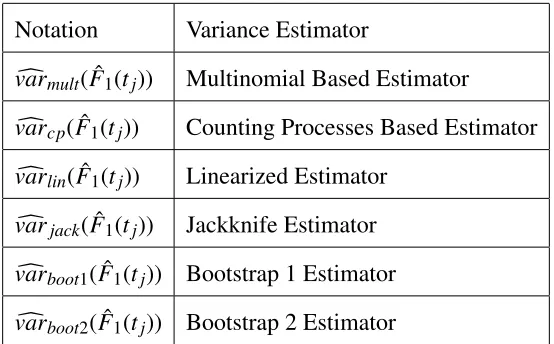
data and extended them to the clustered competing risks setting. The six variance estimators in

Table 2.1 along with confidence intervals constructed from them will be compared via

simula-tion study. The design of this study is described in Chapter 3 and the results are presented in

(27)

Table 2.1: Variance Estimators

Notation Variance Estimator

c

varmult( ˆF1(tj)) Multinomial Based Estimator

c

varcp( ˆF1(tj)) Counting Processes Based Estimator

c

varlin( ˆF1(tj)) Linearized Estimator

c

varjack( ˆF1(tj)) Jackknife Estimator

c

varboot1( ˆF1(tj)) Bootstrap 1 Estimator

c

(28)

Chapter 3 Design of the Simulation Study

3.1 Introduction

In this chapter we describe the design of the simulation study, making sure to include all the

relevant components discussed by Burton et al. (2006). There are seven sections in this chapter,

including this introduction. Section 3.2 justifies selection of parameters for the generation of

data used in the simulation study. Then Section 3.3 outlines the study design while Section 3.4

and 3.5 describe the model and method by which datasets are generated. Section 3.6 describes

the criteria used to evaluate the methods of confidence interval construction and finally, Section

3.7 briefly summarizes the key elements of study design.

3.2 Parameters

The simulated datasets are designed to replicate an arm from a cluster randomized trial

where patients from different centers are followed for 5 years until one of two competing

events occurs or they are administratively censored due to trial completion. That is, all clusters

and subjects are recruited prior to random assignment. This is done for simplicity of data

gen-eration and to avoid potential for selection bias. We are interested in estimating the cumulative

incidence of the event of interest at study completion along with variances and 95% confidence

intervals. Where possible, values for parameters will be motivated by data from the two studies

mentioned in the Introduction: bone marrow transplant data discussed by Zhou et al. (2012)

(29)

Chapter 3. Design of the Simulation Study 21

and prostate cancer data described by Messing et al. (1999). The parameters specified to

gener-ate the simulgener-ated datasets are: the cumulative incidence, the hazard rgener-ate for the event of interest

and for the competing risk, the percentage of patients censored, the intracluster correlation

co-efficient (ICC), the number of patients enrolled in the study, the size of each cluster. We will

generate datasets based on concrete values for these parameters and calculate the cumulative

incidence at 5 years.

The cumulative incidence is determined by specifying the hazards of the event and

com-peting risk and the percentage of censoring. Based on our choices for these parameters, the

simulation was conducted for cumulative incidence values of approximately: 0.25, 0.33, 0.37,

0.4, 0.54, and 0.6.

The hazard of a patient experiencing any event is determined by the percentage of events

censored, fixing the sum of the hazards of the study outcome and the competing event. In

specifying hazard rates of the event of interest and the competing risk, we wish to model

scenarios where, like our motivating datasets described in the introduction, the event of interest

occurs more often than the competing event. A constant hazard rate for both risks is also

assumed. This may not be a large disadvantage; Chen et al. (2008) conducted a simulation

study examining the bias of a cumulative incidence estimator under clustering and found the

results with time varying hazards didn’t significantly differ from those with fixed hazards. The

ratio of patients experiencing the event of interest to the competing risk is between 1 and 3 in

both motivating datasets and is completely determined by the ratio of their hazards. We will

consider scenarios where the ratio is either 1, 2, or 3.

Attention is limited to administrative censoring, that is, censoring due to not all patients

experiencing an event at 5 years when the cumulative incidence is calculated. We assume that

all clusters and patients within clusters are enrolled prior to the start of the study. We adjusted

the range of the censoring variable so that the percentage of observations censored is on average

20% or 50%.

(30)

are from different centers (Donner and Klar 2000). Recall an ICC=0 indicates no intracluster

correlation while an ICC=1 means total dependence between responses from the same cluster.

Thus we considered ICC values of 0.01, 0.05 and as a check an ICC of 0 as well.

We are interested in scenarios where there are either 400 or 100 patients enrolled in a

study. In the motivating studies described in the Introduction, because the diseases are rare

in the general population, the number of patients recruited per center is low and the number

of centers is high. For simplicity, we considered cases where the same number of patients is

recruited from each cluster. For the case when 100 patients are enrolled, cluster sizes of 5,

10, and 20 are chosen. This will give us scenarios where there are 5, 10, and 20 clusters from

which patients are recruited. For the case when 400 patients are enrolled, cluster sizes of 10,

40, and 80 will be used. This will give scenarios where there are 5, 10, and 40 clusters from

which patients are recruited.

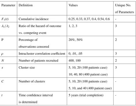
The values of the parameters to be investigated are summarized in Table 3.1. Using these

parameter values there are 3×2×3×2×3=3322=108, scenarios to investigate.

3.3 Simulation Procedures

For each scenario, 1000 independent datasets were generated and each of the methods of

variance construction are applied to each dataset. The estimated cumulative incidence and the

estimated variance estimators for each dataset were stored.

In the exceptional case that a dataset has only censored data (i.e. when there are no events

in a dataset), it will be replaced. The probability of this happening is less than (1/2)100because

the probability of an individual observation being censored is less than 1/2.

The simulation study was conducted using R version 3.2.0 (R Core Team, 2015). The

generation of random numbers was done using the “runif”, “rbin”, “rexp”, and “rgamma”

functions from the base package. A starting seed was specified for each scenario to ensure that

scenarios are independent of each other and can be replicated. To further aid in replication, the

(31)

Table 3.1: Simulation Parameters

Parameter Definition Values Unique No.

of Parameters

F1(t) Cumulative incidence 0.25, 0.33, 0.37, 0.4, 0.54, 0.6

-λ1/λ2 Ratio of the hazard of outcome 1, 2, 3 3

vs. competing event

P Percentage of 20%, 50% 2

observations censored

ρ Intracluster correlation coefficient 0, .01, .05 3

N Number of patients recruited 400, 100 2

s Cluster size 5, 10, 20 (100 patients case) 3

10, 40, 80 (400 patient case)

C Number of clusters 5, 10, 20 (100 patients case)

-5, 10, and 40 (400 patient case)

t Time confidence interval 5 years (trial completion)

(32)

3.4 Modeling the Data

We will model the clustering effect using a shared gamma frailty model. The relationship

between the ICC and the frailty parameter is given by Jeong and Jung (2006). For our purposes,

it suffices to note that givenC clusters, frailties v1,...,vC generated from a single-parameter

gamma distribution with shapeρand scale 1/ρ, model a within cluster correlation ofρ. Thus

we generateCfrailtiesv1,...,vC from the model shown in Equation (3.1).

f(v;ρ)= v ρ−1_eρv

Γ(ρ)(1/ρρ) v>0, ρ >0 (3.1) Then for each cluster c, independent event times follow an exponential distribution with hazardvc(λ1+λ2), conditional on the shared frailty.

3.5 Data Generation Procedure

Some investigators simulate competing risks data using a latent failure time model (e.g.

Illjon (2013), Braun and Yuan (2007)). As described in the Introduction, we use only

ob-servable quantities for the analysis of competing risks, to minimize model assumptions. Thus

we prefer the approach of Beyersmann (2009) over the latent failure approach. Beyersmann

(2009)’s approach is described in our data generation algorithm below.

The data are generated so observations from the same cluster are correlated. The procedure

for data generation based on the specified parameters is as follows:

1. Generate frailties, v1,...,vC, from a single-parameter gamma distribution with shape ρ

and scale 1/ρ, which implies a within cluster correlation with the ICC,ρ.

2. We wish to generate data so that at time t=5 years on average P percent experience neither event (i.e are censored). To do this, we must determine a value for the hazard

of experiencing either event (i.e. λ1+λ2). Because we have a fixed timet=5, a fixed probability that P percentage of events are greater than 5, and event times follow an exponential distribution, we can determine a value forλ1+λ2. Then we can determine

(33)

3. For each cluster cgenerate sevent times from an exponential distribution with hazard

vc(λ1+λ2). We now have observations (tc1,...,tcNc) wheretciis the time of the event, for

i∈ {1,...,Nc}.

4. After event times are generated for each cluster, assign to each event time an

asso-ciated risk δc1,...,δcNc, where these can either take the value 1 or 2 to indicate the time is associated with the event or the competing risk respectively. These are

gener-ated from a binomial random variable, with the event assigned probabilityλ1/(λ1+λ2)

and the competing event assigned probability λ2/(λ1+λ2). We now have observations

(tc1,δc1),...,(tcNc,δcNc).

5. If a timetci exceeds 5, replace its value with 5 and replace the value for δc1 with 0, to indicate it has been administratively censored.

6. Return observations (tc1,δc1),...,(tcNc,δcNc) forc∈ {1,...,C}.

3.6 Evaluation Criteria

The primary purpose of the simulation study is to evaluate the confidence interval

estima-tors constructed from the variance estimaestima-tors described in Section 2.3, but we will also test the

performance of the variance estimators, as these are the variable component of the different

methods of confidence interval construction.

3.6.1 Criteria to Assess Variance Estimators

Following Braun and Yuan (2007) and Chen et al. (2008), we compare the mean variance

of each estimator to the empirical variance.

3.6.1.1 Percentage Bias of Estimated Variance

Given 1000 simulated datasets, and the prespecified timet=5, we obtain estimators of the cumulative incidence ( ˆF1(t)i)1000_i₌₁ . The empirical variance will be given by the formula:

E MV := 1000

X

i=1

(34)

where ¯ˆF1(t)i=P1000_i₌₁

ˆ

F1(t)i 1000.

The percentage bias is then approximated by the percentage difference between the

empir-ical variance and the mean of a variance estimator over the different simulations. It is given

by:

[₁₀₀₀1 P1000

i=1 varc( ˆF1(t)i)]−E MV

E MV (3.3)

We consider a percentage bias of magnitude over 15% to be a poor performance by a

variance estimator.

3.6.2 Criteria to Assess Confidence Interval Estimators

We evaluate the confidence interval estimators on coverage and width. The latter is done by

examining the width of the estimated confidence intervals, and the former by whether the true

value of the cumulative incidence was in the confidence interval or missed to the left or right

of the interval. Because the confidence interval estimators are for the cumulative incidence

function, which in general is bounded by [0,1], if we estimate a lower bound below 0 or an

upper bound above 1 they will be truncated to 0 or 1 respectively. This will have to be done

with the linear method of confidence interval construction only, not the log-log method, which

always gives results within these bounds.

3.6.2.1 Coverage

The confidence interval estimators will be examined by determining the proportion of times

the confidence interval contained the true value of the cumulative incidence function at the

specified point in time. The true value of the cumulative incidence function will be given by

F1(t)= Z t

u=0

λ1S(u)du (3.4)

whereS(t)=exp−Rt

u=0(λ1+λ2)du

.

For a given scenario, variance estimator and method of confidence interval construction, let

(35)

of timesF1(t) is in the confidence interval is:

#{F1(t)∈[Li,Ui] :i=1,...,1000}

1000 (3.5)

A better performance is, all things equal, indicated by the proportion being closer to 95%.

More specifically, following the method of Bradley (1978), we consider coverage outside the

bounds set by 0.95±1.96√0.95×(0.05/1000), which is approximately between 93.5% and

96.5% to be poor.

We also consider the proportion of times the true value of the cumulative incidence function

misses to the left and to the right. These are respectively:

#{F1(t)<[Li,Ui] :i=1,...,1000}

1000 (3.6)

and

#{F1(t)>[Li,Ui] :i=1,...,1000}

1000 (3.7)

It is preferable to have symmetry in proportion of misses to the left and right.

3.6.2.2 Width

To assess the precision of the confidence interval estimators we calculate their average

length over the simulated datasets. This is:

1 1000

1000 X

i=1

(Ui−Li) (3.8)

The shorter the length of an estimator, the more precise the estimator will be. It is expected

that methods that account for clustering, due to this, will have greater coverage but also greater

width. If two estimators perform similarly in coverage, but one has a shorter width on average,

(36)

3.7 Summary

The simulation study to be performed compares six variance estimators of the cumulative

incidence, listed in Table 2.1, and the twelve confidence interval estimators built from these

variance estimators. It compares them over a range of scenarios described in Section 3.2. The

scenarios are motivated by the datasets described in Chapter 1 and analyzed in detail in Chapter

5.

Data will be simulated by the method given by Beyersmann (2009) to limit attention only

to the modeling of observable quantities.

The variance estimators are compared on their percentage bias and the methods of

(37)

Chapter 4 Results of the Simulation Study

4.1 Introduction

Section 4.2 provides general remarks about the simulation and describes the manner in

which the results are presented. Section 4.3 discusses the percentage bias performance of the

variance estimators while Section 4.4 discusses the performance of the confidence interval

estimators. Section 4.5 summarizes the main findings of this chapter and Section 4.6 contains

tables of the simulation results.

4.2 Description of Simulation Results

Recall that 1000 replications were performed for each of the 108 scenarios distinguished

by the parameters listed in Table 3.1. For each scenario, the cumulative incidence and the six

variance estimators summarized in Table 2.1 were estimated. These variance estimators were

the Multinomial Based Estimator, Counting Processes Based Estimator, Linearized Estimator,

Jackknife Estimator, a cluster-sample Bootstrap Estimator, and a two-step Bootstrap Estimator.

They are denoted Mult, CP, Lin, Jack, Boot1, and Boot2 respectively and are described in

Chapter 2.

The performance of these variance estimators and the confidence intervals formed from

them was evaluated as described in Section 3.6. First, the percentage bias of the variance

estimators was calculated. Then, for both the linear and log-log methods of confidence interval

(38)

Chapter 4. Results of the Simulation Study 30

construction, and each of the six variance estimators, coverage, left and right misses, and mean

confidence interval width were calculated. Recall from Section 3.3 that we would resimulate a

dataset in the event that it contained only censored observations, as this would make the use of

a cumulative incidence estimator impossible. This simulation had no occurrence of a dataset

containing only censored observations and thus no resimulation was needed.

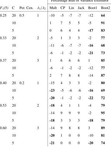
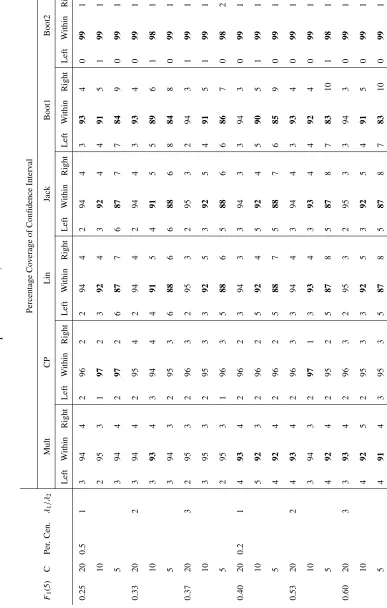
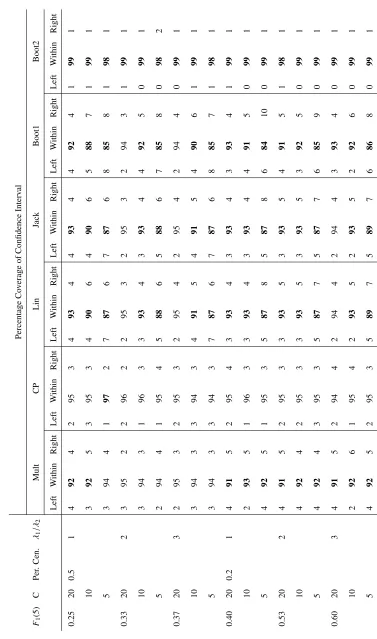
All simulation results are presented at the end of this chapter in Section 4.6. The simulation

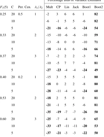
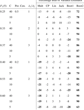
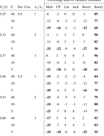
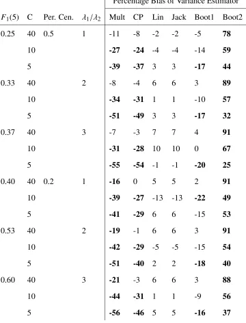
results for the percentage bias of the variance estimators are presented in Tables 4.1 to 4.6.

While we discuss both the linear and log-log methods of confidence interval construction in

this chapter, only the coverage of the confidence intervals (including left and right misses)

formed using the log-log method are presented. These are given in Tables 4.7 to 4.12. The

reason we do not present the tables for the linear method of confidence interval construction is

given in Section 4.4. We also present in Tables 4.13 to 4.18, the average width of the log-log

estimators.

Thus in Section 4.6, where we present the results of the simulation, there are three sets of

tables for the 108 scenarios: one set for the percentage bias results, one set for the coverage of

the log-log interval estimators, and one set for the width of the log-log interval estimators. For

readability, each set of results is presented in six tables containing 18 scenarios (6x18=108),

organized as follows: the first three tables are simulations where the total sample size was 100,

the latter three where the total sample size was 400. For a fixed total sample size, each table

presents the results for those scenarios where the ICC was 0, 0.01, or 0.05 respectively.

Thus a table contains, for a fixed total sample size and ICC, the results for the 18 scenarios

created by taking all possible values of the remaining parameters of data generation. These

were the value of the cumulative incidence att=5 (i.e. F1(5)), the number of clustersC, the percentage of observations censored, and the ratio of the hazards of the event of interest and

the competing risk (i.e.λ1/λ2).

Finally, we note one particularity of the results. Despite the Linearized and Jackknife

(39)

biases were indistinguishable and their coverage performance were identical regardless of use

of the linear or log-log method of confidence interval construction.

4.3 Percentage Bias Results

This section discusses the the percentage bias simulation results of the variance estimators.

These results are displayed in the tables Table 4.1 to Table 4.6. In these tables, those cases

where a method had above 15% absolute bias were bolded.

We first examine the number of scenarios in which a variance estimator has the lowest

ab-solute percentage bias. The Linearized and Jackknife variance estimators achieved the lowest

absolute percentage bias the most number of times, in 54 of the 108 scenarios, while the

Count-ing Process estimator achieved it the second most at 43. The Multinomial estimator achieved

it under 10 times and the Bootstrap 1 estimator 14 times. Bootstrap 2 never had the lowest

percentage bias.

Next we examine the percentage of scenarios for which an estimator has absolute

percent-age bias ≤15%. The Linearized and Jackknife estimator satisfy this 100% of the time. The

Counting Processes estimator 81% and Bootstrap 1 at 69%, and Multinomial estimator 44% of

times. Bootstrap 2 never achieves absolute bias under 15%.

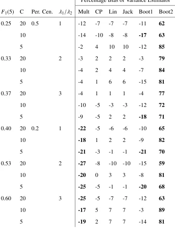
We now consider the influence varying each parameter has on the absolute percentage bias

of each variance estimator. As the ICC, ρ, increases the bias of Multinomial and Counting

Process estimators increase, which is to be expected as these estimators do not account for

clustering. The Linearized, Jackknife, and Bootstrap 1 estimators all have no noticeable change

in bias, while the bias of the Bootstrap 2 estimator decreases as clustering increases.

AsN, the total sample size, increases from 100 to 400, the Multinomial and Counting Pro-cess estimators increase in percentage bias, while other estimators show no noticeable change.

This is likely due to an increase in the clustering effect, as those cases whenN=400 generally have larger clusters.

(40)

As the number of clustersCincreases, the absolute percentage bias generally decreases for all but the Bootstrap 2 estimator. The bias for the Linearized and Jackknife estimators, seems

unaffected by the number of clusters increasing.

The percentage censored changing from 20% to 50%, appears not to have an effect except to

decrease the mean absolute percentage bias for the Multinomial estimator. Changing the ratio

of the hazards of the event of interest and competing risk has no clear effect on the percentage

bias results.

4.4 Confidence Interval Results

This section discusses the performance of the confidence intervals formed from the variance

estimators. First we compare the performance of the linear and log-log methods of confidence

interval construction. Because the log-log method provides better coverage, we will consider in

greater detail the coverage and width performance of the confidence interval estimators using

the log-log method.

The coverage of the log-log confidence intervals for all scenarios are displayed in Table 4.7

to Table 4.12. In these tables, as discussed in Section 3.6.2.1, those cases where the coverage

was approximately between 93.5% and 96.5% were thought to have good coverage. Instances

outside this range are bolded.

4.4.1 Di

ff

erence Between Linear and Log-Log Methods of Confidence

In-terval Construction

We compared the size of the difference in overall coverage between the linear and log-log

confidence interval methods, for each of the 108 scenarios and 6 variance estimators. Thus

there were 6×108=648 total comparisons of coverage performance. The difference in

cover-age between them exceeds 2% only 19 times in total (approx 3% of the cases). In no case did

the difference in coverage between the linear and log-log exceed 3%.

For each method of variance estimation, we compared the number of scenarios where a

(41)

interval is constructed using the linear versus using the log-log method. This nearly always

increased when the log-log method was used; increasing by 8 for the Multinomial estimator,

by 4 for the Linearized and Jackknife estimator and by 5 when Bootstrap 1 is used. The number

of scenarios with acceptable coverage decreased by 1 when Bootstrap 2 is used. Because of

it’s better performance, we only present tables of coverage and width for the log-log method

of confidence interval construction.

4.4.2 Confidence Interval Performance

We now examine in greater detail, for only the log-log method of confidence interval

con-struction, the performance of the different confidence interval estimators.

In 77 of 108 scenarios the Counting Process method provided coverage in our acceptable

range. It is the only method that had acceptable coverage in over 50% of the scenarios. Of

course, a third of our scenarios had no clustering effect whatsoever. Indeed, in scenarios with

ICC of 0.05, it often performs significantly worse than Bootstrap 2.

Thus we will consider the influence varying the parameters ICC, sample size, number of

clusters, and the value of the cumulative incidence has on the coverage of each variance

esti-mator.

When the ICC is 0 the Counting Process estimator should clearly be preferred over the

other estimators. Although when F1(5) is smaller, the Multinomial estimator has slightly bet-ter coverage. As the ICC, ρ, increases from 0 to 0.01, there is no great difference between

coverage in any of the estimators. However as the ICC increases from 0.01 to 0.05, the number

of scenarios with good coverage drops for both the Multinomial and Counting Processes

esti-mators, which is to be expected, as these do not account for clustering. Even whenρ=0.05, the

Linearized, Jackknife and Bootstrap 1 estimators never achieve the required number of clusters

and sample size to outperform the Counting Processes estimator when the sample size is 100.

However, when the sample sizeN=400 andρ=0.05, these estimators sometimes offer better coverage than Counting Process estimator. The Bootstrap 2 performs well in 4 scenarios where

(42)

andC=5. This suggests that in scenarios where there is a small number of large clusters and heavy clustering, the Bootstrap 2 may be the preferred estimator.

When the number of clusters C is less than or equal to 10, the Linearized, Jackknife and Bootstrap 1 estimators rarely have acceptable coverage, but when they are above 10, they have

good coverage a number of times comparable to the Counting Process method, even under no

clustering.

For estimators accounting for clustering there was no noticeable pattern that increasing the

value ofF1(5) had on coverage performance. However the Multinomial estimator performed better for lower values ofF1(5) and the Counting Process estimator performed better for higher values.

The coverage of the confidence interval estimators varied significantly. As such, diff

er-ences in left and right misses between estimators is not as valuable a consideration as if the

performance of estimators was closer.

The average width of estimators corresponds with the coverage performance of the esti-mators. As expected, increasing the number of clusters does not change the average width of

a confidence interval estimators not account for clustering. The width of the Bootstrap 2 had

the widest average width over all scenarios, whose coverage was also always the largest. The

Bootstrap 1 width was always lower than the Linearized and Jackknife widths.

4.5 Summary of Simulation Results

This simulation study found that the percentage bias of the Linearized and Jackknife

esti-mators was lowest, but this did not correspond to their having good confidence interval

cov-erage. This is perhaps because we examined many scenarios with a number of clustersC too small for their asymptotic performance to be noticeable.

The log-log method of confidence interval construction is to be preferred to the linear

method.

The Counting Process estimator was clearly the best performer under no clustering and

(43)

is 100. However, under clustering of 0.05 and a sample size of 400, methods accounting for

clustering showed better coverage. With a sample size of 400 and a low number of large

clusters (i.e. 5 clusters of 40 patients each), the Bootstrap 2 method performs the best.

Confidence Interval Estimation of Cumulative Incidence for Clustered Competing Risks

Scholarship@Western

Scholarship@Western

Confidence Interval Estimation of Cumulative Incidence for

Confidence Interval Estimation of Cumulative Incidence for

Clustered Competing Risks

Clustered Competing Risks

Abstract

Acknowledgments

Contents

List of Figures

List of Tables

List of Abbreviations

Chapter 1

Introduction

1.1

The Competing Risks Setting

1.2

Focus of Thesis

1.3

Objectives of Thesis

1.4

Organization of Thesis

Chapter 2

Literature Review

2.1

Introduction

2.2

Thesis Setting

2.3

Notation

2.4

Competing Risks Estimators

2.4.1

Estimating the Cumulative Incidence Function

2.4.2

Variance Estimators Under Independence

2.4.3

Extending Williams’ Linearized Variance Estimator

2.4.4

Bootstrap Variance Estimators

2.4.5

Jackknife Variance Estimator

2.5

Confidence Interval Estimates

2.6

Summary

Chapter 3

Design of the Simulation Study

3.1

Introduction

3.2

Parameters

3.3

Simulation Procedures

3.4

Modeling the Data

3.5

Data Generation Procedure

3.6

Evaluation Criteria

3.6.1

Criteria to Assess Variance Estimators

3.6.2

Criteria to Assess Confidence Interval Estimators

3.7

Summary

Chapter 4

Results of the Simulation Study

4.1

Introduction

4.2

Description of Simulation Results

4.3

Percentage Bias Results

4.4

Confidence Interval Results

4.4.1

Di

ff