Efficient Localization Algorithm of Mixed Far-Field and Near-Field
Sources Using Uniform Circular Array
Bing Xue1, 2, *, Guangyou Fang1, 2, and Yicai Ji1, 2
Abstract—An efficient algorithm based on high-order cumulant is addressed for the scenarios where both far-field and near-field narrow-band signals may exist synchronously. The first matrix built by four-order cumulant is utilized to estimate the two dimensional direction-of-arrivals (DOAs) using the orthogonal projection matrix of the signal subspace and the virtual steering matrix. Then, the second matrix built by four-order cumulant is decomposed to get the noise subspace using the eigen decomposition. Meanwhile, a virtual steering matrix is used to distinguish far-field signals (FFSs) from near-field signals (NFSs). And one-dimensional MUSIC algorithm is used to estimate the range of the NFSs. Compared to the TSMUSIC, the proposed algorithm can provide high resolution for the DOAs. In addition, there is higher accuracy for the DOA of NFS in the proposed algorithm than that in TSMUSIC and in TSMD. Simulation results are carried out to certify the performance of the proposed algorithm.
1. INTRODUCTION
There has been considerable interest in the passive sources localization with an array of spatially separated sensors, which has many important application areas such as radar, guidance systems and sonar [1]. Various high performance algorithms such as MUSIC [2] and ESPRIT [3] have been used to deal with the DOA estimation of the FFSs. However, the both DOA and range of the source that is localized at the Fresnel region of the array aperture need be considered in some practical applications like lightening localization and speaker guidance systems [4], each source may be in the near field or the far field of the sensor position. Hence, when the classical algorithms may fail in such scenarios, several solutions are available to process the mixed sources localization. Using two high dimensional cumulant matrices of the sensor outputs, Liang and Liu [4] provided a two-stage MUSIC algorithm to solve the mix sources localization problem of the high resolution, which has high computational complexity and cannot classify the FFSs and NFSs in similar DOA. Wang et al. [5] used the mixed-order MUSIC algorithm to decline the computational complexity and improved the accuracy. Jiang et al. [6] gave an algorithm that estimates DOAs of all FFSs and NFSs by ESPRIT, distinguishes the FFSs and NFSs and estimates the range of NFSs by MUSIC. Liu and Sun [7] used the spatial differencing technique to classify the NFSs from the mixed sources after the estimations of FFSs, which has the higher accuracy, classify the mixed signals successfully and lower computational load. The algorithm in [8] built the optimization problem to get the estimation function used to obtain the DOA and estimated the range of the source by the minimum variance distortionless response (MVDR). Yet, the aforementioned high resolution algorithms are all aimed at two dimensional localization (elevation DOA and range). For some three dimensional problems (azimuth angle, elevation angle and range), they may fail in mixed sources localization so that we need to have an increase for the performances.
Received 24 August 2016, Accepted 14 October 2016, Scheduled 30 October 2016
* Corresponding author: Bing Xue ([email protected]).
Recently, there is a significant amount of attention paid to the three dimensional localization (two dimensional DOA). Two parallel uniform linear arrays (ULAs) were used in [9] to estimate the two-dimensional direction (azimuth angle, elevation angle) for noncoherent and coherent signals by the orthogonal projector. An L-shaped ULA was used in [10] to estimate the two dimensional DOAs for noncoherent signals using a computational efficient subspace-based algorithm. Wu et al. [11] presented multiple near-field sources localization using the two-stage MUSIC (TSMUSIC) by UCA. And Jung and Lee [12] gave an easy way to calculate the three-dimensional information of a single source. UCA is preferable over uniform linear array because of its 360◦azimuthal coverage, additional angle information and unchanged directional pattern [11] for estimating mixed sources. So, in this paper, we choose the UCA to estimate the mixed source locations. The novel solution includes three stages: 1) UCA is used to estimate the mixed sources three dimensional localization. We give the mathematical model for this situation, which is similar to the model in [11–13]. 2) Two useful four-order cumulant matrices for UCA are built to distinguish the NFSs and FFSs, which can realize a more reasonable classification of the signals types than correlation function. 3) The virtual steering matrices are built to estimate the DOAs and the ranges, respectively. And the orthogonal projector is used in MUSIC, which can provide the great estimation accuracy and low computing complexity.
2. MIXED FAR-FIELD AND NEAR-FIELD SIGNAL MODEL
We consider the narrow-band signals (NF far-field signals and NN near-field signals) impinging on a UCA [11] with radius R and M identical omnidirectional sensors, and the array center is the phase reference point. Without loss of the propagation, all the sensors are employed on the xy-plane, while the FFSs are located at (θi, ϕi) and the NFSs located at (θi, ϕi, ri), whereθi ∈[0,2π) are the azimuth angles measured counterclockwise from the x axis; ϕi ∈ [0, π/2) are the elevation angles measured downward from the z axis; ri is the range measured from the UCA centre and i = 1,2, . . . , N. The received signal of the UCA by the k-th sensor can be expressed as
xk(t) =
NN
i=1
si(t)ej2λπ{ri−rk(θi,ϕi,ri)}+
NN+NF
i=1+NN
si(t)ej2λπRψk,i(θi,ϕi)+n(t) (1)
where k= 1,2, . . . , M, si(t) is the i-th source signal, n(t) the additive sensor noise, and ψk,i(θi, ϕi) = cos(γk−θi) sin(ϕi) with γk = 2πk/M being the angle of the k-th sensor measured counterclockwise from thex-axis. λis the wavelength of the source and rk(θi, ϕi, ri) the distance between thei-th source and thek-th sensor, which can be written as
rk(θi, ϕi, ri) =
r2
i −R2−2riRψk,i(θi, ϕi) (2)
According to the Taylor series expansion, Eq. (2) can be approximated as
rk(θi, ϕi, ri)≈ri−Rψk,i(θi, ϕi) +R 2
2ri
1−ψ2k,i(θi, ϕi) (3)
whereRr, substituting Eq. (3) into Eq. (1) yields
xk(t) =
NN
i=1
si(t)e j2πR
λ
ψk,i(θi,ϕi)−2Rri(1−ψk,i2 (θi,ϕi))
+
NN+NF
i=1+NN
si(t)ej2λπRψk,i(θi,ϕi)+n(t) (4)
In matrix form, Eq. (1) can be written as
x(t) =ANSN(t) +AFSF(t) +n(t) (5)
wherex(t) and n(t) areM×1 dimensional complex vectors.
AN = [aN(θ1, ϕ1, r1),aN(θ2, ϕ2, r2), . . . ,aN(θNN, ϕNN, rNN)] (6)
AF = [aF(θ1, ϕ1),aF(θ2, ϕ2), . . . ,aF(θNF, ϕNF)] (7)
aN(θ, ϕ, r) = [ej2λπR{ψ1(θ,ϕ)−2Rr(1−ψ12(θ,ϕ))}, . . . , ej2λπR{ψM(θ,ϕ)−2Rr(1−ψ2M(θ,ϕ))}]T (8)
where ψk(θ, ϕ) = cos(γk−θ) sin(ϕ), k= 1,2, . . . , M. Eqs. (8) and (9) represent the steering vector of NFSs and FFSs, respectively. And the superscriptT denotes the transpose operator. In addition, the assumptions are required to point out. The source signals are statistically independent processes, which are also independent from the source signals. For the rest of this paper, the following assumptions are need to hold:
1) The source signals are statistically mutually independent, uncorrelated narrowband stationary processes.
2) The sensor noise is spatially uniform white and independent from the signals.
3. THE PROPOSED ALGORITHM
In this section, we will give the algorithm which estimates DOAs of all FFSs and NFSs firstly, then classifies the FFSs and NFSs and estimates the ranges of NFSs lastly.
3.1. DOA Estimation of the Far-Field and Near-Field Sources
For the MUSIC algorithm using high-order cumulant to estimate DOAs of all signals, we should build a new cumulant of the sensor outputs. Assume that M is even, and the four-order cumulant is used to make the cumulant matrix, which can be shown in Eqs. (8)–(11):
C11 = cum
xp(n)x∗M/2+p(n)x∗q(n)xM/2+q(n)
=
NN+NF
i=1
C4,iej4πRλ {ψp,i(θi,ϕi)−ψq,i(θi,ϕi)} (10)
C12 = cum
xp(n)x∗p−M/2(n)x∗q(n)xM/2+q(n)
=
NN+NF
i=1
C4,iej4πRλ {ψp,i(θi,ϕi)−ψq,i(θi,ϕi)} (11)
C13 = cum
xp(n)x∗M/2+p(n)x∗q(n)xq−M/2(n)
=
NN+NF
i=1
C4,iej4πRλ {ψp,i(θi,ϕi)−ψq,i(θi,ϕi)} (12)
C14 = cum
xp(n)x∗p−M/2(n)x∗q(n)xq−M/2(n)
=
NN+NF
i=1
C4,iej4πRλ {ψp,i(θi,ϕi)−ψq,i(θi,ϕi)} (13)
where C4,i = cum{si(t)s∗i(t)s∗i(t)s(it)} is the four-order cumulant of the i-th signal; the superscript ∗ represents the complex conjugate; n= 1,2, . . . , Np represents snapshot number.
Here,p ∈[1, M/2] and q ∈[1, M/2] for Eq. (10), p ∈[1 +M/2, M] and q ∈[1, M/2] for Eq. (11), p∈[1, M/2] andq ∈[1 +M/2, M] for Eq. (12), p∈[1 +M/2, M] and q∈[1 +M/2, M] for Eq. (13).
We can only estimate the DOAs of the signals withoutr in Eqs. (10)–(13). C11,C12,C13andC14 that are all the (M/2)×(M/2) matrices are combined into a matrix. This M×M matrix C1 can be constructed as follows:
C1 =
C11 C13
C12 C14 =
G1
H1 (14)
whereG1 is a ¯K×M matrix, andH1 is a (M−K¯)×M matrix. We can use the virtual steering matrix to estimate the DOAs, which can be written as
AV1 = [a(θ1, ϕ1), . . . ,a(θNN+NF, ϕNN+NF)] (15)
a(θi, ϕi) =
ej4πRλ ψ1,i(θi,ϕi), . . . , ej4πRλ ψM,i(θi,ϕi)T (16)
AV1 is aM×(NF +NN) matrix. Using Eq. (15), Eq. (14) can be expressed as
C1=AV1CsAHV1= ¯
A1
¯ A2 Cs
¯
A1
¯ A2
H
¯
A1 is a ¯K×M matrix, andA¯2 is a (M−K¯)×M matrix. The superscriptH is the conjugate transpose operator. Equivalently,A¯2=PαnA¯1. Then,Pαn can be obtained.
ˆ
Pαn=G1GH1 −1
G1HH1 (18)
We can easily get
EαnAV1 =O (19)
where Eαn = [PˆTαn −IT]T,I∈CM−K×M−¯ K¯ is an identity matrix, and O is a zero matrix. Evidently, the columns of Eαn form a basis of the null space of AV1, so the orthogonal projector is expressed as
Uαn =EαnEHαnEαn−1EHαn (20)
which is used to obtainUHαnAV1=O. When the finite snapshots of array data are available, the DOAs of all signals can be estimated by the minimizing argument of the cost function:
f1(θ, ϕ) =aH(θ, ϕ)UαnUHαna(θ, ϕ) (21)
wherea(θ, ϕ) = [ej4πRλ ψ1(θ,ϕ), . . . , ej4λπRψM(θ,ϕ)]T.
3.2. Distinction of the Far-Field and Near-Field Sources
For distinguishing the FFSs and NFSs, we need to build the second cumulant matrixC2, which is used to estimate the ranges of the NFSs. To utilize signal information adequately, aM×M matrix is built using the four-order cumulant. Here,p∈[1, M] andq ∈[1, M] for Eq. (22).
C2 = cumxp(n)x∗M(n)x∗q(n)xM(n)
=
NN
i=1
C4,ie j2πR
λ
ψp,i(θi,ϕi)−ψq,i(θi,ϕi)−2R
ri(ψ2p,i(θi,ϕi)−ψ2q,i(θi,ϕi))
+
NN+NF
i=1+NN
C4,iej2λπR(ψp,i(θi,ϕi)−ψq,i(θi,ϕi)) (22)
Using eigenvalue decomposition,C2 can be written as
C2=Σs2UsΣHs2+Σn2UnΣHn2 (23)
where the (NF+NN)×(NF+NN) matrixUscontains the (NF+NN) signal subspace eigenvalues ofC2, and theM×(NF+NN) matrixΣs2 spans the signal subspace ofC2. In turn, theM×(M−NF−NN) matrixΣn2 spans the noise subspace ofC2. Generally, the eigenvalues of the signal subspace are larger than those of the noise subspace.
Before estimating the ranges of the NFSs, we should select the NFSs from all of the signals. Assume that all of the signals are the FFSs. Using the MUSIC algorithm, we put all of DOA estimated by Eq. (21) into Eq. (24). When f2(ˆθi,ϕˆi)0, thei-th signal is the FFS. On the contrary, this signal is the NFS.
Here,bsH(θ, ϕ) is the virtual steering matrix that is the same as Eq. (9).
f2θ,ˆ ϕˆ=bsH(ˆθ,ϕ)ˆ U
nUHnbs(ˆθ,ϕ)ˆ
−1
(24)
3.3. Range Estimation of the Near-Field Signals
It is clear that 1D-MUSIC algorithm like Eq. (25) can be used to estimate theri(i= 1,2, . . . , NN) since ˆ
θi and ˆϕi have been obtained.
f3θˆi,ϕˆi, ri=asHθˆi,ϕˆi, riUnUH
nas
ˆ θi,ϕˆi, ri
−1
(25)
4. COMPUTER SIMULATION RESULTS
In this section, some simulation results are given to evaluate the performance of the proposed algorithm. For the first and second examples, an eight-sensor symmetric UCA with R = λ is given. Two equal power narrowband signals (one NFS and one FFS) are impinging on this array. The additive noise is supposed to be spatial white complex Gaussian random process. And the signal-to-noise ratio (SNR) is defined relative to each signal. For the comparison, we execute the TSMUSIC [11] using Rk,l =E{xkxl∗}(k, l= 1,2, . . . , M) by eigen value decomposition (EVD), which estimates firstly DOAs of all FFSs and NFSs and then estimates the ranges of NFSs, execute the TSMD [7] that distinguishes firstly the FFSs and NFSs and then estimates the locations of FFSs and NFSs respectively, and execute the related Cramer-Rao Bound (CRB). The results shown next are evaluated by the estimated root man square error (RMSE) from the average results of 200 independent Monte-Carlo simulations.
In the first experiment, we consider the simulation that there are a NFS and a FFS incoming on the sensor array, and their DOAs are similar ((152.1◦, 33.2◦) and (160.3◦, 33.2◦, 6.1λ)). The SNR and the snapshot number are set at 20 dB and 1200, respectively. The spatial spectrum of the proposed algorithm and TSMUSIC [11] is shown in Fig. 1. From this figure, the proposed algorithm gives the two peaks for these two signals, which successfully yields DOA estimations for both NFS and FFS. However, the TSMUSIC [11] only gives a peak for these two signals, that is, which cannot give the right DOA for the NFS so that it is invalid for the similar DOAs of two signals. So, our algorithm can achieve a more reasonable classification for the signals than TSMUSIC [11].
50 100 150 200 250 300 350
-10 0 10 20 30 40 50
DOA in degree
S
pat
ia
l S
pec
tr
um
i
n
dB
the proposed method azimuth TSMUSIC azimuth
Figure 1. Spatial spectrum of azimuth estimation. (152.1◦, 33.2◦) and (160.3◦, 33.2◦, 6.1λ), SNR = 10 dB, the snapshot number is 2000.
0 2 4 6 8 10 12 14 16 18 20
-30 -25 -20 -15 -10 -5 0 5 10
SNR (dB)
RM
S
E
(d
egre
e) i
n
d
B
proposed method FFS azimuth proposed method NFS azimuth TSMUSIC FFS azimuth TSMUSIC NFS azimuth TSMD FFS azimuth TSMD NFS azimuth CRB FFS azimuth CRB NFS azimuth
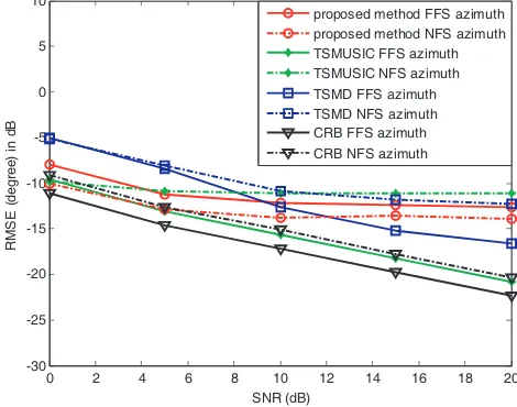
Figure 2. RMSEs of azimuth angles estimations for mixed NFSs and FFSs versus SNRs. (82.5◦, 33.2◦) and (160.3◦, 62.1◦, 6.1λ), the snapshot number is 2000. 200 independent trails.
0 2 4 6 8 10 12 14 16 18 20 -30 -25 -20 -15 -10 -5 0 5 10 15 SNR (dB) R M S E ( d egree) in d B
proposed method FFS elevation proposed method NFS elevation TSMUSIC FFS elevation TSMUSIC NFS elevation TSMD FFS elevation TSMD NFS elevation CRB FFS elevation CRB NFS elevation
Figure 3. RMSEs of elevation angles estimations for mixed NFSs and FFSs versus SNRs. (82.5◦, 33.2◦) and (160.3◦, 62.1◦, 6.1λ), the snapshot number is 2000. 200 independent trails.
0 2 4 6 8 10 12 14 16 18 20
-30 -25 -20 -15 -10 -5 0 5 10 SNR (dB) R M S E (range) in d B
proposed method NFS range TSMUSIC NFS range TSMD NFS range CRB NFS range
Figure 4. RMSEs of range estimations for mixed NFSs and FFSs versus SNRs. (82.5◦, 33.2◦) and (160.3◦, 62.1◦, 6.1λ), the snapshot number is 2000. 200 independent trails.
0 2 4 6 8 10 12 14 16 18 20
-30 -25 -20 -15 -10 -5 0 5 10 15 20 SNR (dB) R M S E (degree)
proposed method FFS azimuth 1 proposed method FFS azimuth 2 proposed method FFS azimuth 3 proposed method NFS azimuth 1 proposed method NFS azimuth 2 proposed method NFS azimuth 3
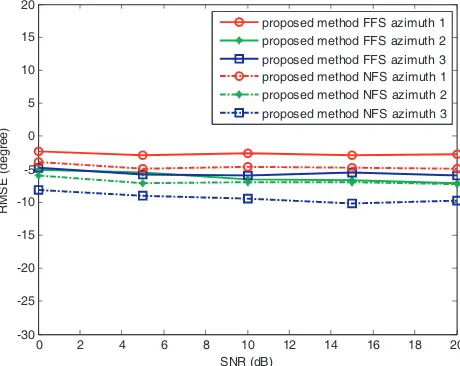
Figure 5. RMSEs of azimuth angles estimations for mixed NFSs and FFSs versus SNRs. (22.10◦, 33.20◦), (61.74◦, 41.06◦, 2.5λ), (101.38◦, 48.92◦, 3.2λ), (141.02◦, 56.78◦, 4.1λ), (180.66◦, 64.64◦) and (220.03◦, 72.50◦). The snapshot number is 2000. 200 independent trails.
0 2 4 6 8 10 12 14 16 18 20
-30 -25 -20 -15 -10 -5 0 5 10 15 20 SNR (dB) R M S E ( d egree) i n d B
proposed method FFS elevation 1 proposed method FFS elevation 2 proposed method FFS elevation 3 proposed method NFS elevation 1 proposed method NFS elevation 2 proposed method NFS elevation 3
Figure 6. RMSEs of elevation angles estimations for mixed NFSs and FFSs versus SNRs. (22.10◦, 33.20◦), (61.74◦, 41.06◦, 2.5λ), (101.38◦, 48.92◦, 3.2λ), (141.02◦, 56.78◦, 4.1λ), (180.66◦, 64.64◦) and (220.03◦, 72.50◦). The snapshot number is 2000. 200 independent trails.
0 2 4 6 8 10 12 14 16 18 20 -30
-25 -20 -15 -10 -5 0 5 10 15 20
SNR (dB)
R
M
S
E
(
range)
i
n
dB
proposed method NFS range 1 proposed method NFS range 2 proposed method NFS range 3
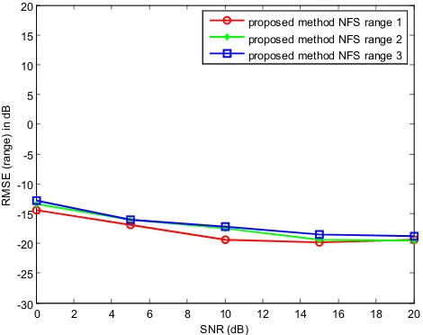
Figure 7. RMSEs of range estimations for mixed NFSs and FFSs versus SNRs. (22.10◦, 33.20◦), (61.74◦, 41.06◦, 2.5λ), (101.38◦, 48.92◦, 3.2λ), (141.02◦, 56.78◦, 4.1λ), (180.66◦, 64.64◦) and (220.03◦, 72.50◦). The snapshot number is 2000. 200 independent trails.
5. COMPUTATIONAL COMPLEXITY
For the computational complexity, we consider the major multiplications existing in matrix construction, EVD computation, and MUSIC spectrum search. The TSMUSIC method [11] contains one M ×M matrix, performs its EVD, and needs one two-dimensional DOA search and NN times range search. Hence, the multiplications are estimated by
O
M2N
p+43M3+360δ
θ 180
δϕ M 2+N
NLenδ
r M
2
(26)
whereNp represents the snapshot number;δθandδϕdenote the search step of DOA;δris the search step of range;Lenis the length of range search. The TSMD method [7] contains oneM×M matrices, builds one difference matrix, executes the EVD of two matrices, as well as performs twice two-dimensional DOA search andNN times range search. Hence, the multiplications are estimated by
O
M2N
p+ 2M2+83M3+ 2360δ
θ 180
δϕ M 2+N
NLenδ
r M
2
(27)
Similarly, the proposed method contains two M ×M matrices, executes the EVD of one matrix, as well as performs twice two-dimensional DOA search and NN times range search. Hence, the multiplications are estimated by
O
3M2Np+4 3M
3+ 2360 δθ
180 δϕ M
2+N
NLenδ
r M
2
(28)
We can find that the TSMUSIC method [11] has the lowest computational complexity, and the proposed method has higher computational complexity than the TSMUSIC method [11] and TSMD method [7].
6. CONCLUSIONS
REFERENCES
1. Krim, H. and M. Viberg, “Two decades of array signal processing research: The parametric approach,”IEEE Signal Processing Magazine, Vol. 13, No. 4, 67–94, 1996.
2. Schmidt, R. O., “Multiple emitter location and signal parameter estimation,” IEEE Transactions on Antennas and Propagation, Vol. 34, No. 3, 276–280, 1986.
3. Rot, R. and T. Kailath, “Esprit-estimation of signal parameters via rotational invariance techniques,” IEEE Transactions on Acoustics, Speech, and Signal Processing, Vol. 37, No. 7, 984– 995, 1989.
4. Liang, J. and D. Liu, “Passive localization of mixed near-field and far-field sources using two-stage music algorithm,”IEEE Transactions on Signal Processing, Vol. 58, No. 1, 108–120, 2010.
5. Wang, B., Y. Zhao, and J. Liu, “Mixed-order MUSIC algorithm for localization of far-field and near-field sources,”IEEE Signal Processing Letters, Vol. 20, No. 4, 2013.
6. Jiang, J., F. Duan, J. Chen, Y. Li, and X. Hua, “Mixed near-field and far-field sources localization using the uniform linear sensor array,”IEEE Sensors Journal, Vol. 13, No. 8, 3136–3143, 2013. 7. Liu, G. and X. Sun, “Two-stage matrix differencing algorithm for mixed far-field and near-field
sources classification and localization,” IEEE Sensors Journal, Vol. 14, No. 6, 1957–1965, 2014. 8. Xie, J., H. Tao, X. Rao, and J. Su, “Passive localization of mixed far-field and near-field sources
without estimating the number of sources,” Sensors, Vol. 15, No. 15, 3834–3853, 2015.
9. Tao, H., J. Xin, J. Wang, N. Zheng, and A. Sano, “Two-dimensional direction estimation for a mixture of noncoherent and coherent signals,” IEEE Transactions on Signal Processing, Vol. 63, No. 2, 318–333, 2015.
10. Wang, G., J. Xin, N. Zheng, and A. Sano, “Computationally efficient subspace-based algorithm for two-dimensional direction estimation with L-shaped array,” IEEE Transactions on Signal Processing, Vol. 59, No. 7, 3197–3212, 2011.
11. Wu, Y., H. Wang, Y. Zhang, and Y. Wang, “Multiple near-field source localisation with uniform circular array,”Electronics Letters, Vol. 49, No. 24, 1509–1510, 2013.
12. Jung, T. and K. Lee, “Closed-form algorithm for 3-D single-source localization with uniform circular array,”IEEE Antennas Wireless Propagation Letters, Vol. 13, No. 6, 1096–1099, 2014.