The Second Order Finite Element Analysis of Eddy Currents
Based on the T-
Ω
Method
Bo He*, Ping Zhou, Dingsheng Lin, and Chuan Lu
Abstract—Based on a proposed inexact Hodge decomposition, this paper describes a viable scheme using the second order finite elements in the T-Ω method considering multiply-connected regions for the eddy current problems. Several numerical examples have been presented to demonstrate the effectiveness of this scheme.
1. INTRODUCTION
The numerical simulations of eddy currents have a wide range of low-frequency electromagnetic applications which include induction furnaces, electrical machines, eddy-current brakes, magnetic levitation, electromagnetic launching, biomedicine, nondestructive testing, and so on [1]. Based on the finite element method, the T-Ω method is one of the most effective methods for the numerical analysis of eddy currents [2]. In this method, the magnetic field intensity is expressed as the sum of two parts: the gradient of a magnetic scalar potential Ω and electric vector potential T. In order to maintain tangential continuity, the electric vector potential can be interpolated by Whitney edge elements [3]. However, these elements are low-order vector basis functions and give a poor convergence to the induced eddy current density because the induced eddy current density, which is the curl of T, is only a piecewise constant vector in the finite element approximation. Better convergence can be achieved using higher-order vector elements. Although several higher-order vector elements have been developed in literature [4], it is still not a trivial task to construct a viable scheme for the T-Ω method using higher order vector elements. A T-Ω method using the higher order hierarchical scalar and vector basis functions has been proposed in [3], but assumes that the problem domain is only simply-connected. Since the magnetic scalar potential Ω may be multivalued, handling the multiply-connected domains in the T-Ω method is indispensable. Based on a proposed inexact Hodge decomposition, a viable scheme using the second vector order finite elements to interpolate the electric vector potential considering multiply-connected regions was described briefly in [5]. In this paper, we will discuss this scheme extensively, and demonstrate its effectiveness by presenting several numerical results.
2. THE T-Ω METHOD
In frequency domain, the equations for the eddy current problem can be written in terms of the magnetic field intensityH in the whole region
∇ ×H =J (1)
∇ ·μ H
= 0 (2)
Received 16 December 2014, Accepted 2 March 2015, Scheduled 10 March 2015
* Corresponding author: Bo He ([email protected]).
and the conducting region
∇ × 1
σ∇ ×H +jμω H= 0 (3)
where J is the impressed source current density, μ the permeability, ω the angular frequency, and σ
the conductivity. By introducing the electric vector potential for source currentHp, the electric vector potential for the induced current T and the magnetic scalar potential Ω, the magnetic field intensity can be expressed as following
H=∇Ω +T+Hp. (4)
Plugging (4) into (2) and (3) and moving the source terms to the right hand sides, we have the eddy current equations in terms of the electric vector potential and the magnetic scalar potential
∇ ·(μ∇Ω) =−∇ ·
μ Hp
(5)
∇ × 1
σ∇ ×T+jμω
∇Ω +T
=−∇ × 1
σ∇ ×Hp−jμω Hp (6)
The major advantages of the above formulation are (a) the computational cost is reduced with the use of the magnetic scalar potential in the whole domain and (b) it is easier to handle the moving objects thanA-phi formulation [1].
Now consider how to obtain the electric vector potential for source currentHp by the finite element method. The electric vector potential for source currentHp satisfies the Amp`ere’s law
∇ ×Hp =J (7)
In differential form language, the magnetic field intensity Hp is a 1-form, and the current density J
is a 2-form. Whitney forms are the basic interpolants for the different forms defined over tetrahedra. Whitney 1-form and 2-form can be expressed in terms of barycentric coordinates ςi, ςj, ςk associated with each tetrahedron vertex as [6, 7]
wij =ςi∇ςj−ςj∇ςi, (8)
wijk =ςi∇ςj× ∇ςk+ςk∇ςi× ∇ςj+ςj∇ςk× ∇ςi, (9)
In the above the interpolant wij is defined on the edge connecting vertices iandj, and the interpolant
wijk is defined on the face connecting vertices i, j and k, respectively. Accordingly, we use Whitney
1-form as the interpolant for the magnetic field intensityHp and Whitney 2-form as the interpolant for the current densityJ, i.e.,
Hp=
hijwij (10)
J =jijkwijk (11)
Plugging (10) and (11) into (7), we have the discrete version of (7)
[d] [Hp] = [J] (12)
3. HODGE DECOMPOSITION
Applying the Hodge decomposition to the magnetic field intensity 1-form H gives
H =dφ+δA+χ, (13)
where φis a magnetic scalar potential 0-form,A a 2-form, χ the harmonic field component, and dthe exterior derivative, andδ the codifferential operator, the adjoint ofd[9]. The codifferential δ operator can be expressed as [10]
δ =∗−1d∗, (14)
where∗ is the Hodge star operator. The operatorsdand δ satisfy
dd=δδ= 0 (15)
The finite element approximation of (14) gives the matrix formulation
[δ] = [∗]−1[d] [∗], (16)
where [d] is the incidence matrix and [∗] the mass matrix. Although [d] and [∗] are sparse matrices, [δ] is generally a full matrix because the inverse of [∗] is a full matrix. This implies that δ is not a local operator althoughdis a local operator. Correspondingly, it is not necessary for the basis of the electric vector potential T to be divergence-free. Instead, we will use rotational basis functions as introduced in [3, 11], which may not be exactly divergence-free, to interpolateT. Since the rotational basis functions are not necessarily divergence-free in a finite element setting, this decomposition of vector basis into the gradient of a scalar basis and the rotational vector basis is termed the inexact Hodge decomposition.
4. BASIS FUNCTIONS
The lowest vector basis function to interpolateT is the Whitney edge element. As a result, the induced eddy current density, which is the curl of T, is only a piecewise constant vector in the finite element approximation. In order to obtain a more accurate eddy current density distribution, higher order vector basis functions may be needed. In the literature there are two types of vector basis: the interpolatory basis and the hierarchical basis [4, 12]. The interpolatory vector basis functions are defined on a set of interpolation points on the element and their coefficients have a physical interpretation as components of the vector fields at the interpolation points [4]. However, the interpolatory vector basis functions with different orders cannot be used together since the interpolatory vector basis functions of a higher order are not explicitly constructed on those of the lower orders. The hierarchical vector basis functions are not defined on a set of interpolation points, but defined on the edges, faces and volumes of the element. Since the hierarchical vector basis functions of a higher order explicitly contain lower order basis functions, it allows mixing of different order vector bases. Because of the above property, it can handle the harmonic field component naturally. This will be detailed in the next section. The hierarchical second order vector basis functions are as follows [3, 13]:
w1ij =ςi∇ςj−ςj∇ςi, (17)
w2ij =ςi∇ςj+ςj∇ςi, (18)
fijk =ςkςj∇ςi, (19)
The basis functions (17) and (18) are defined on the edge connecting vertices i and j, and the basis function (19) is defined on the face connecting vertices i,j and k [13]. Note that although both vector basis functionsfijk and wijk are defined on faces, they are quite different. One is the interpolant for the
The basis function (18) can be expressed as the gradient of the scalar basis function
w2ij =∇(ςiςj) (20)
Since (20) is a pure gradient basis function, it can represent the first term of (13). The gradient of the second order scalar basis functions interpolating the magnetic scalar potential Ω also contain ∇(ςiςj). Therefore, the vector basis function (18) in the T-Ω method is redundant and can be recycled, and only the rotational basis functions (17) and (19) are needed to interpolate T.
5. MULTIPLY-CONNECTED REGIONS
In the T-Ω method, if the conductors contain holes, the region is connected. In the multiply-connected region, the harmonic field component χ will not be zero. The harmonic field component χ
has the properties
dχ= 0 (21)
δχ= 0, (22)
which means that the harmonic field is both curl-free and divergence-free. As discussed in [15], one cannot construct any vector basis that should be simultaneously curl-free and divergence-free. However, it is still possible to construct a vector basis that is locally divergence-free and globally curl-free. Since generally the interpolatory high order vector bases do not satisfy divergence-free condition, we shall choose candidates from the hierarchical high order vector basis functions. It can be shown that
∇ ·wij1 =∇ ·(ςi∇ςj−ςj∇ςi) = 0, (23)
∇ ·fijk =∇ ·(ςkςj∇ςi)= 0, (24)
That is, the Whitney edge element (17) is free while the face element (19) is not divergence-free. Therefore, the basis function for the harmonic field component should be the Whitney edge element. Once the Whitney edge element is chosen as the basis for the harmonic field component, (22) is automatically satisfied, and then only (21) should be satisfied. Precisely, in the finite element method, the discrete version of (21)
[d] [χ] = [0] (25)
should be satisfied. In (25), [χ] is the column vector and [d] is the incidence matrix. Note that the dimension of the column vector [χ], which is the degree of freedom (DOF) of the harmonic field component, is the number of loops, so it is independent of the mesh and orders of the basis functions.
There are several approaches to model (21), the topological property of the harmonic field component [15–23]. Reference [23] introduced an efficient cut-generating algorithm with computational complexityO(N2) whereN denotes the number of DOF’s in the finite element discretization. The
thick-cut, which is one layer of tetrahedral elements having their edges passing through cutting surfaces, as introduced in [15, 16] has the computational complexity O(N1.5) or less for most practical simulations.
Also, thick-cut can be naturally adapted to Hp assignment procedure. Therefore, in this paper the thick-cut will be applied to model the harmonic field component. The thick-cut can be generated by the following two steps [16]:
Step 1. Make surface cuts on the surface of conducting regions. Scan all triangles on the conductor surfaces and for each triangle examine whether each edge forms a loop or not. The triangle with all three edges connected will be added to the set of singly connected surfaces. This process is repeated until there are no more triangles to be added. The rest of the triangles that do not belong to the set of singly connected surfaces create surface cuts on the conductor surfaces.
6. NUMERICAL EXAMPLES
TEAM (Testing Electromagnetic Analysis Methods) [24] provides a list of test-problems, which can be used to validate the computational method and algorithm. Here we use two TEAM examples to verify the effectiveness of the proposed method.
6.1. TEAM 7
TEAM 7 is a thick conductor plate with a hole placed unsymmetrically in a non-uniform magnetic field. The field is generated by sinusoidal current with frequency 200 Hz. Since there is a hole in the thick conductor plate, it is a multiply-connected region problem. Figure 1 presents the generated mesh of plate which is used in the FEM calculations. Figure 2 presents the calculated induced eddy current densities. Note that the induced eddy current density calculated by the second order vector basis functions is much smoother than that calculated by the first order vector basis functions. Figure 3 presents the calculated induced eddy current densities along the lines A3-B3and A4-B4. Refer to [24, 25]
for the definition of those lines. The magnitudes displayed in Figure 3 are invariably the magnitudes of the complex functions, which may be positive or negative, indicating the direction of the currents [25]. Note that the magnitudes of Jy along the line A4-B4 drop rapidly because of the skin effect of eddy
currents. These results clearly demonstrate that the second order vector basis functions produce more accurate current density than the first order vector basis functions.
The Ohmic loss due to the induced eddy current can be calculated by
P =
vol
J ·J
2σ dv (26)
Figure 1. The mesh of the plate.
(a) (b)
(a) (b)
Figure 3. (a) Magnitude ofJy along the line A3-B3. (b) Magnitude of Jy along the line A4-B4.
Table 1. Losses and relative errors of the conductor plate of TEAM 7.
Number of tetrahedrons
Loss (W) (the first order )
Loss (W) (the second order)
Relative error (the first order)
Relative error (the second order)
3325 8.6980 9.4900 0.1180 0.0377
6325 9.0080 9.8150 0.0866 0.0047
11369 8.9200 9.5930 0.0955 0.0273
25578 9.3530 9.7700 0.0516 0.0093
62239 9.6570 9.8270 0.0208 0.0035
Table 2. Losses and relative errors of TEAM 21.
Models Measured Loss (W)
Loss (W) (the first order)
Loss (W) (the second order)
Relative error (the first order)
Relative error (the second order)
P21a-1 3.40 3.29 3.35 0.0324 0.0147
P21a-2 1.68 1.59 1.70 0.0536 0.0119
For this example, neither measured Ohmic loss nor analytical solution is available to compare. In order to calculate the relative errors of the Ohmic loss, we choose a reference loss as the accurate solution. This reference loss is calculated by using the first order vector basis functions with a very refined mesh with 443458 tetrahedrons for the conductor plate. The relative loss errors are obtained by calculated losses against the reference loss. Table 1 presents the calculated losses and relative errors of the conductor plate. The results show that the second order vector basis functions produce more accurate Ohmic loss than the first order vector basis functions.
Since the DOF of the vector basis functions is defined only on the induced eddy current region, the DOF of the whole computational domain using the second order vector basis functions does not increase significantly. For this example, the DOFs using the first order vector basis functions and using the second order vector basis functions are 20835 and 32671, respectively.
6.2. TEAM 21
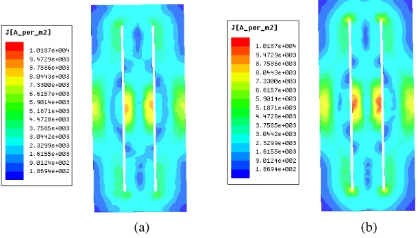
TEAM 21 includes 15 member models. Here we only choose two models, P21a-1 and P21a-2, which are linear eddy current problems and multiply-connected region problems since they have slots on the plates. In these models, the exciting source is composed of two identical coils with the electric currents flowing in opposite directions. The exciting current is set to 3000 A (rms, 50 Hz). Figure 4 presents the calculated induced eddy current densities of P21a-2.
(a) (b)
Figure 4. (a) The induced eddy current density calculated by the first order vector basis functions (Whitney elements). (b) The induced eddy current density calculated by the second order vector basis functions.
7. CONCLUSIONS
In this paper, in order to construct a viable scheme of a second order T-Ω method, we propose an inexact Hodge decomposition. With the help of the inexact Hodge decomposition, we propose a second order T-Ω method, which can be applied to handle the multiply-connected regions naturally. In this method, the hierarchical second order vector basis functions are used to interpolate the electric vector potential of induced eddy current; the Whitney edge elements are used to interpolate the harmonic field component; the Whitney edge elements are used to interpolate the electric vector potential of the impressed source currents; the second order interpolatory basis functions are used to interpolate the scalar potential Ω. The numerical results have verified the effectiveness of the second order T-Ω method.
REFERENCES
1. Kriezis, E. E., T. D. Tsiboukis, S. M. Panas, and J. A. Tegopoulos, “Eddy currents: Theory and application,”Proceedings of the IEEE, Vol. 80, No. 10, 1559–1589, Oct. 1992.
2. Prenston, T. W. and A. B. J. Reece, “Solution of 3-D eddy current problems: The T-Omega method,”IEEE Trans. Magn., Vol. 18, 486–491, 1982.
3. Webb, J. P. and B. Forghani, “A T-Omega method using hierarchal edge elements,” Proc. Inst. Elec. Eng. Sci. Meas. Technol., Vol. 142, No. 2, 133–141, Mar. 1995.
4. Jin, J., The Finite Element Method in Electromagnetics, Wiley-IEEE Press, 2002.
5. He, B., P. Zhou, D. Lin, and C. Lu, “High order finite elements in T-Ω method considering multiply-connected regions,” Compumag Conference, 5–20, 2013.
6. Bossavit, A., “Whitney forms: A class of finite elements for three-dimensional computations in electromagnetism,” IEE Proc., Vol. 135, No. 3, 179–187, 1988.
7. He, B. and F. L. Teixeira, “Compatible diecretizations for Maxwell equations,” VDM Verlag, 28, 2009.
8. Webb, J. P. and B. Forghani, “A single scalar potential method for 3D magnetostatics using edge elements,” IEEE Trans. Magn., Vol. 25, 4126–4128, 1989.
9. He, B. and F. L. Teixeira, “On the degree of freedom of lattice electrodynamics,” Phys. Lett. A, Vol. 336, 1–7, 2005.
11. Lee, S., J. Lee, and R. Lee, “Hierarchical vector finite elements for analyzing waveguiding structures,”IEEE Trans. on Microwave Theory and Techniques, Vol. 51, No. 5, 1897–1905, 2003. 12. Ren, Z., “Application of differential forms in the finite element formulation of electromagnetic
problems,” ICS Newsletter, Vol. 7, No. 3, 6–11, 2000.
13. Webb, J. P. and B. Forghani, “Hierarchal scalar and vector tetrahedra,” IEEE Trans. Magn., Vol. 29, 1495–1498, 1993.
14. Zienkiewicz, O. C., R. L. Taylor, and J. Z. Zhu, The Finite Element Method: Its Basis and
Fundamentals, Butterworth-Heinemann, 2006.
15. Kettunen, L., K. Forsman, and A. Bossavit, “Discrete spaces for div and curl-free fields,” IEEE Trans. Magn., Vol. 34, 2551–2554, 2002.
16. Ren, Z., “T-Ω formulation for eddy current problems in multiply connected regions,” IEEE Trans. Magn., Vol. 38, 557–560, 2002.
17. Demenko, A. and J. K. Sykulski, “Network representation of conducting regions in 3D finite element description of electrical machines,” IEEE Trans. Magn., Vol. 44, No. 6, 714–717, 2008.
18. Wojciechowski, R. M., A. Demenko, and J. K. Sykulski, “Inducted currents analysis in multiply connected conductors using reluctance-resistance networks,” COMPEL: The International Journal for Computation and Mathematics in Electrical and Electronic Engineering, Vol. 29, No. 4, 908–918, 2010.
19. Dlotko, P. and R. Specogna, “Lazy cohomology generators: A breakthrough in (co)homology computations for CEM,”IEEE Trans. Magn., Vol. 50, No. 2, 577–580, 2014.
20. Simkin, J., S. C. Taylor, and E. X. Xu, “An efficient algorithm for cutting multiply connected regions,”IEEE Trans. Magn., Vol. 40, No. 2, 707–709, 2004.
21. Phung, A. T., O. Chadebec, P. Labie, Y. Le Floch, and G. Meunier, “Automatic cuts for magnetic scalar potential formulations,” IEEE Trans. Magn., Vol. 41, No. 5, 1668–1671, 2005.
22. Crager, J. C. and P. R. Kotiuga, “Cuts for the magnetic scalar potential in knotted geometries and force-free magnetic fields,” IEEE Trans. Magn., Vol. 38, No. 2, 1309–1312, 2002.
23. Gross, P. W. and P. R. Kotiuga, “Finite element-based algorithms to make cuts for magnetic scalar potentials: Topological constraints and computational complexity,” Geometric Methods for Computational Electromagnetics, Vol. 32, 207–245, 2001.
24. http://www.compumag.org/jsite/team.html.
25. Biro, O., K. Preis, W. Renhart, K. R. Ritcher, and G. Vrisk, “Performance of different vector potential formulations in solving multiply connected 3D eddy current problems,” IEEE Trans. Magn., Vol. 26, 438–441, 1990.