A Virtual Space-Time Adaptive Beamforming Method
for Space-Time Antijamming
Fulai Liu1, *, Ruiyan Du1, *, and Xiaoyu Bai2
Abstract—Space-time antijamming problem has received significant attention recently in the passive radar systems, such as Global Navigation Satellite Systems (GNSS). The space-time beamformer contains two adaptive filters, i.e., spatial filter and temporal filter for canceling interference signals. However, most of the works on space-time antijamming problem presented in the literature require multiple antennas and delay taps. In this paper, a virtual space-time adaptive beamforming method is proposed. The temporal smoothing technique is utilized to add a structure of the received data model for the implementation of the proposed method without delay taps. Compared with the previous works, the presented method offers a number of advantages over other recently proposed algorithms. For example, the space-time weight vector can be obtained by simple algebraic operations with lower computational complexity, since the matrix inversion is avoided. Furthermore, the system overhead can be reduced obviously since the temporal smoothing technology is used instead of multiple delay taps. Simulation results are presented to verify the effectiveness of the proposed method.
1. INTRODUCTION
Adaptive beamforming is a method for receiving the interested signal of specific direction while
suppressing the jamming signals of other directions through an array of antennas. The minimum
variance distortionless response (MVDR) algorithm is one of the popular approaches, which minimizes the array output power while maintains a distortionless mainlobe response [1]. Unfortunately, the MVDR beamformer may have unacceptably high sidelobes, which may lead to significant performance degradation in the case of unexpected interfering signals [2]. A large number of robust beamforming methods based on MVDR have been presented later [2–9]. For example, covariance matrix tapers and derivative constraints are used in [2]. White noise gain constraint is considered in [3]. Space-time averaging techniques and rotation techniques of the steering vectors are proposed in [4]. A new method based on amplitude-only perturbations is given in [5]. A multi-parametric quadratic programming method is presented in [6], and a blind adaptive beamforming method called power inversion is proposed in [7] for low signal-noise-ratio (SNR) scenario. Additionally, the genetic algorithm (GA) is considered in [8] and [9]. The algorithm in [8] aims at adaptively eliminating interfering signals, and an enhanced GA method is proposed in [9] to synthesize planar, sparse and aperiodic arrays.
However, in general, the adaptive beamforming method above can only process N −1 jamming
signals using an N-element array. To overcome the shortcoming, temporal degrees of freedom are also employed, and a space-time processor is introduced, leading to the space-time adaptive processing (STAP) technique [10]. In STAP, multiple delay taps, which can be regarded as a finite impulse response (FIR) filter, are placed after each sensor, and it can process many more narrowband interference sources than the number of sensors via the temporal degrees of freedom [11, 12]. In STAP, the dimension equals
Received 3 May 2017, Accepted 8 July 2017, Scheduled 19 July 2017
* Corresponding author: Fulai Liu ([email protected]), Ruiyan Du ([email protected]).
1 Engineer Optimization & Smart Antenna Institute, Northeastern University at Qinhuangdao, China.2School of Computer Science
the product of the number of antenna elements and the order of the FIR filter. The STAP methods have found numerous applications in modern systems encountered in communications [13], radar [14], and navigation [15–17].
Numerous algorithms with different tradeoffs between performance and complexity for designing STAP have been proposed [18–24]. A STAP method with sub-band structure, called sub-band adaptive
array (SBAA) is put forward in [18, 19]. The SBAA can make parallel processing at high speed
and reduce the computational complexity. A rank-reducing STAP algorithm is proposed in [20].
The rank-reducing STAP method does not require matrix inversion and has a lower computational complexity. Another method to reduce the computational complexity without severely affecting the performance is spatial frequency adaptive processing, which transfers the temporal domain processing to frequency domain processing through the Fourier transform or bandpass filter [21]. A robust space-time beamforming based on second-order cone programming is presented in [22]. In the presented method, all the line-of-sight signals are pointed by the array, and the temporal reference of the signal is exploited. The work also presents an extension of this beamforming that takes into account the incertitudes in the steering matrix due to pointing errors or array miscalibration. A multiple constraints space-time beamformer is given by [23]. The proposed space-time beamformer can be operated in multiple linear constraints mode to combat the angle mismatch problem. The antijamming performance of the spatial adaptive processing and STAP is discussed in [24].
However, all of the above space-time beamforming methods require multiple antennas with delay taps which incur high system overhead. In this paper, an effective virtual space-time beamforming method is proposed. The temporal smoothing technique is utilized to add a structure of the received data model for the implementation of proposed method based on multiple antennas without delay taps. The proposed approach makes use of the Frame method to obtain the inverse matrix to avoid the complexities of matrix inversion. The rest of the paper is organized as follows. The data model is described in Section 2. Section 3 introduces the presented method. Section 4 shows some simulation results. Finally, the conclusion is given in Section 5.
2. DATA MODEL
Consider a uniform linear array (ULA) ofM elements equispaced by d. Employing the first element of the ULA as the phase reference, the array manifold can be written as
aM(f, θ) =
1, ejμ, . . . , ej(M−1)μ
T
(1)
where μ = (2πf /c)dsin(θ) with f and θ denoting the frequency and direction of arrival (DOA), respectively. c stands for the velocity of light. dis equal to the interelement spacing.
Suppose that there are q narrowband sources of interest, with complex baseband representations si(t), for i= 1, . . . , q. Suppose that theith source has a carrier frequency of fi. The signal received at thekth antenna is [25]
xk(t) = q
i=1
ak(fi, θi)ej2πfitsi(t) +wk(t) (2)
whereak(fi, θi) is the antenna response of thekth antenna to the signal from the directionθi, andwk(t)
represents the output of the additive noise of thekth sensor. The observed signals at the ULA are given by
x(t) =As(t) +w(t) (3)
The matrices and vectors in Eq. (3) have the following forms
x(t) = [x1(t),· · · , xM(t)]T
A = [aM(f1, θ1),· · ·,aM(fq, θq)] s(t) = [s1(t),· · ·, sq(t)]T
wherexk(t) andwk(t) (k= 1, . . . , M) denote the output signal and the additive noise of the kth sensor, respectively. aM(fk, θk) (k = 1, . . . , q) is the steering vector for the kth source, which is defined by
Eq. (1). The superscript (·)T represents the transpose operation. Assume that wk(t) is a complex
Gaussian random process with zero-mean and variance σn2, and the noise wk(t) is uncorrelated with si(t).
Under the above assumptions, it can be easily seen that E{w(t)wH(t)} = σn2IM where E{·} represents the statistical average operation, and the superscript (·)H denotes the Hermitian operation.
IM is theM ×M identity matrix.
Assume that P is the sample rate, which is much higher than the data rate of each source. The data samples at the receiver are
x n P = q i=1
a(fi, θi)ej(2π/P)finsi
n P +w n P (4)
In matrix form, it can be written as
x n
P
=AΦns n P +w n P (5)
where Φ = diag{(φ1, . . . , φq)} with φi = ej(2π/P)fi for i = 1, . . . , q, which includes the information of
the frequencies of incident signal sources, e.g., we refer matrixΦas time factor matrix and its diagonal element as time factor. Assume that we have collected N samples of the array outputx(t) at a rateP into theM ×N data matrix, i.e.,
X n P =A
s(0),Φs
1
P , . . . ,Φ N−1s
N −1
P +W (6)
whereW is a matrix collecting N samples of the M×1 array noise vector.
3. ALGORITHM FORMULATION
3.1. Temporal Smoothing
Consider a data stacking technique, which is referred as temporal smoothing. An m-factor temporal smoothed data matrix is constructed by stacking m temporally shifted versions of the original data matrix. This results in the followingmM ×(N−m+ 1) matrix
Xm=
⎡ ⎢ ⎢ ⎢ ⎢ ⎢ ⎢ ⎢ ⎢ ⎢ ⎢ ⎣ A
s(0),Φs
1
P , . . . ,Φ
N−msN −m P AΦ s 1 P ,Φs
2 P , . . .
.. .
AΦm−1
s
m−1
P ,Φs
m P , . . . ⎤ ⎥ ⎥ ⎥ ⎥ ⎥ ⎥ ⎥ ⎥ ⎥ ⎥ ⎦
+Wm (7)
where Wm represents the noise term constructed from W in a similar way as Xm obtained from X. Assume that the signals are narrow band, i.e.,s(t)≈s(t+ 1/P)≈. . .≈s(t+ (m−1)/P). In this case, all the block rows in the right-hand term of Eq. (7) are approximately equal, which means thatXm has the following factorization
Xm ≈ ⎡ ⎢ ⎢ ⎣ A AΦ .. .
AΦm−1 ⎤ ⎥ ⎥ ⎦
s(0),Φs
1
P , . . . ,Φ
N−msN −m P
+Wm
whereFs= [s(0),Φs(P1), . . . ,ΦN−ms(N−Pm)]. Am is given by
Am =
⎡ ⎢ ⎢ ⎣
A AΦ
.. .
AΦm−1 ⎤ ⎥ ⎥
⎦=AG
= [aM(f1, θ1)⊗gm(f1), . . . ,aM(fq, θq)⊗gm(fq)] (9)
where A = [aM(f1, θ1), . . . ,aM(fq, θq)], G = [gm(f1), . . . ,gm(fq)] with gm(fk) = [1, φk, . . . , φ(km−1)]T, and ⊗denotes Kronecker product.
3.2. Virtual Space-Time Manifold
Similar to the array response vector aM(f, θ), we can define the virtual space-time response vector
umM(f, θ) as
umM(f, θ) =aM(f, θ)⊗gm(f) (10)
ThismM-dimensional vectorumM(f, θ) is the response of the array to a incoming signal with direction θ and frequencyf. As θ and f vary over the dimensions of angle and frequency, the vector umM(f, θ) traces a multidimensional space-time manifold, which is the combination of the array manifoldaM(f, θ) and the time manifold gm(f), and it is determined by the array geometry, signal frequency and the sampling rate jointly.
Thus, Equation (8) can be rewritten as
Xm =UFs+Wm (11)
whereU=Am= [umM(f1, θ1), . . . ,umM(fq, θq)]. In other words,Uis referred as the virtual space-time
array steering matrix.
Hence, the covariance matrix of them-factor temporal smoothed data matrixXm can be expressed as
Rm=EXmXHm=URsUH +σ2nImM (12)
where the signal covariance matrix Rs =E{s(t)sH(t)}. For the sake of convenience, Rs is assumed to be a full rank matrix, i.e., all sources are not fully correlated.
3.3. The Virtual Space-Time Weight Vector
The virtual space-time beamformer output is given by
y(k) =wHxm(k) k= 1, . . . , N−m+ 1 (13)
wherewis the mM ×1 weight vector, and xm(k) is the kth column vector ofXm.
The MVDR beamformer minimizes the array output power while keeping the unit gain in the desired direction and frequency of the interesting signal
min
w w
HR
mw subject to wHu(f0, θ0) = 1 (14)
whereu(f0, θ0) is the mM×1 virtual space-time steering vector of the desired signal. A closed-form solution to Eq. (14) is given by
wMVDR=
1
u(f0, θ0)HR−m1u(f0, θ0)R
−1
3.4. Frame Method
As discussed above, the inverse R−m1 of Rm is required for calculating the virtual space-time weight vector w. In this subsection, we consider the inverse problem. To reduce the computation cost of the inverse matrix, we use the following Frame algorithm [26].
Summary of Frame method
A1 =Rm, p1= trace(A1), B1 =A1−p1ImM
A2 =A1B1, p2 = 12trace(A2), B2 =A2−p2ImM ..
. ... ...
An=A1Bn−1, pn= n1trace(An), Bn=An−pnImM
⎫ ⎪ ⎪ ⎬ ⎪ ⎪ ⎭
(16)
From the Frame algorithm, it is easy to know that if Rm is a nonsingular matrix, then R−m1 = 1
pnBn−1.
3.5. Summary of the Proposed Method
Step.1 Collect the sample data matrixX according to Eq. (6).
Step.2 Form them-factor temporal smoothed data matrixXm by Eq. (7).
Step. 3 Estimate the covariance matrix ˆRm given by
ˆ
Rm= 1
N−m+ 1
N−m+1
k=1
xm(k)xHm(k)
wherexm(k) denotes thekth volume vector ofXm.
Step. 4 Compute the inverse ˆR−m1 of ˆRm by the Frame method.
Step. 5 Compute the virtual space-time wight vector waccording to Eq. (15).
4. SIMULATION RESULTS
In this section, simulation results are provided to illustrate the performance of the proposed method.
Consider an ULA with M = 5 antenna elements and equispaced by d = 0.125 m. Assume that there
are four far-field signals impinging on the antenna array. Their DOAs are θ1 =−60◦, θ2 = 0◦, θ3 = 30◦, θ4 = 0◦, respectively. Their corresponding center frequencies are f1 = 0.9 GHz, f2= 1 GHz, f3 =
-100 -50
0 50
100
0.5 1
1.5 -60 -50 -40 -30 -20 -10 0 10
DOA(degree) Frequency(GHz)
Response Gain(dB)
Frequency (GHz)
DOA(Degree)
0.6 0.7 0.8 0.9 1 1.1 1.2 1.3 1.4
-80 -60 -40 -20 0 20 40 60 80
interference signal interference signal
desired signal
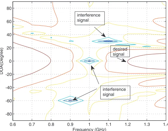
Figure 2. The contour plot of the proposed method.
-100 -80 -60 -40 -20 0 20 40 60 80 100
-60 -50 -40 -30 -20 -10 0 10
DOA (Degree)
Directional pattern (dB)
(0.9,-60) (1.0,0) (1.1,30) (1.2,0)
Figure 3. Direction patterns for different frequency withN = 128, m= 3, andM = 5.
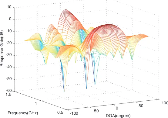
1.1 GHz, f4 = 1.2 GHz, respectively. Their SNRs are equal to snr1 = 25 dB, snr2 = 30 dB,snr3 = 25 dB, snr4 =−10 dB. The sampling rate is set to 4.8 GHz. The number of samples N and temporal smoothing factor mare set to N = 128 andm= 3, respectively.
Figure 1 shows a three-dimensional mesh diagram for space frequency response. In the simulation, the direction and center frequency of the desired signal areθ4 = 0◦ and f4= 1.2 GHz, respectively. The other three signals are interferer signals. As shown in the figure, the weight vector calculated by the proposed method can achieve satisfactory space frequency response performance, such as deeper nulling level.
respectively. That is, the proposed method can suppress the interferer signals effectively and maintain a distortionless response for the desired signal located at (θ4, f4) = (0◦,1.2 GHz).
Figure 3 shows the space response of the proposed approach for different frequency. From this figure, we can observe that a distortionless space response is obtained only at the desired DOA θ4 = 0◦ for the center frequency f4 = 1.2 GHz and three space nulls located at (θ1 =−60◦, θ2= 0◦, θ3 = 30◦), for the center frequencies (f1 = 0.9 GHz, f2= 1GHz, f3 = 1.1 GHz), respectively.
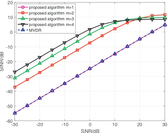
Figure 4 plots the output SINR of the proposed method when the temporal smoothed factor m
varies from 2 to 4. Obviously, (1) the output SINR of the virtual space-time beamforming method is much higher than MVDR. (2) The difference between the performances of the two algorithms is
-30 -20 -10 0 10 20 30
SNR/dB
-60 -50 -40 -30 -20 -10 0 10 20
SINR/dB
proposed algorithm m=1 proposed algorithm m=2 proposed algorithm m=3 proposed algorithm m=4 MVDR
Figure 4. The output SINR versus input SNR for the proposed algorithm and MVDR withN = 128
and M = 5.
0 100 200 300 400 500 600 700 800 900 1000
snapshots
0 2 4 6 8 10 12 14 16 18 20
SINR/dB
proposed algorithm m=1 proposed algorithm m=2 proposed algorithm m=3 proposed algorithm m=4 MVDR
Figure 5. The output SINR versus snapshots for the proposed algorithm and MVDR with input
relatively larger for lower input SNR and becomes smaller when the input SNR is high. (3) The temporal smoothed factor m impacts the output SINR of the proposed method significantly, when the input SNR is low, a larger factormwill bring a better result, but the tendency is just contrary when the input SNR is high. (4) The performance of the virtual space-time beamforming method tends to the
performance of MVDR when m becomes less and less. When m= 1, the two methods are equivalent.
So, the virtual space-time beamforming method can be regarded as the extended version of MVDR at the two dimensions of space and time. In brief, the virtual space-time beamforming method is an improved method based on the MVDR, and it is more appropriate for relatively lower SNR scenario. Additionally, for different input SNRs, the optimal temporal smoothed factor mis different.
Figure 5 shows the influence of snapshots on the output SINR with inputSN R= 30 dB. Evidently, (1) the output SINR of the virtual space-time beamforming method is much higher than MVDR when snapshotsN >50, and the difference between the output SINRs of the two methods becomes larger and larger with the increasing snapshotsN. (2) The temporal smoothed factormimpacts the performance of the virtual space-time beamforming method significantly, and for SN R = 30 dB, smaller factor m brings a better performance, which is consistent with Figure 4. (3) The performance of the virtual
space-time beamforming method with m = 1 is the same as the performance of MVDR, which is also
similar to Figure 4.
5. CONCLUSIONS
In this paper, we present a virtual space-time beamforming method for space-time antijamming problem. The temporal smoothing technique is utilized to add a structure of the received data model such that a virtual space-time array response data can be formed without delay taps. Additionally, the proposed approach makes use of the Frame method to obtain the inverse matrix of the covariance matrix of the temporal smoothed data matrix, so that it avoids the complexities of matrix inversion. Simulations are presented in order to illustrate the performance of the proposed method. It is shown that the presented approach has better space-time antijamming performances than the conventional MVDR method.
ACKNOWLEDGMENT
This work was supported by the Program for New Century Excellent Talents in University (NCET-13-0105), the Support Program for Hundreds of Outstanding Innovative Talents in Higher Education Institutions of Hebei Province, under Grant No. BR2-259, the Natural Science Foundation of Hebei Province (No. F2016501139), the Specialized Research Fund for the Doctoral Program of Higher Education of China (No. 20130042110003), and the Fundamental Research Funds for the Central Universities under Grant (No. N142302001).
REFERENCES
1. Joseph, R. G., “Theory and application of covariance matrix tapers for robust adaptive beamforming,” IEEE Transactions on Signal Processing, Vol. 47, No. 4, 977–985, 1999.
2. Liu, F. L., C. Y. Sun, J. K. Wang, and R. Y. Du, “A robust adaptive beamforming optimization
control method via second-order cone programming for bistatic MIMO radar systems,” ICIC
Express Letters, Vol. 4, No. 5(B), 1823–1830, 2010.
3. Cox, H., R. Zeskind, and M. Owen, “Robust adaptive beamforming,” IEEE Transactions on
Acoustics, Speech, and Signal Processing, Vol. 35, No. 10, 1365–1376, 1987.
4. Liu, F. L., R. Y. Du, J. K. Wang, K. Wang, and B. Wang, “A robust adaptive control method for widening interference nulls,” IET International Radar Conference, 2009.
5. Zeng, Y. B., “Array pattern nulling by amplitude-only perturbations,”Journal of Electronics and Information Technology, Vol. 28, No. 11, 2073–2076, 2006.
7. Wang, Y. D., F. Q. Chen, J. W. Nie, and G. F. Sun, “Optimum reference element selection for GNSS power-inversion adaptive arrays,” Electronics Letters, Vol. 52, No. 20, 1723–1725, 2016. 8. Massa, A., M. Donelli, F. De Natale, S. Caorsi, and A. Lommi, “Planar antenna array control with
genetic algorithms and adaptive array theory,”IEEE Transactions on Antennas and Propagation, Vol. 52, No. 11, 2919–2924, 2004.
9. Donelli, M., S. Caorsi, F. De Natale, D. Franceschini, and A. Massa, “A versatile enhanced genetic algorithm for planar array design,” Journal of Electromagnetic Waves and Applications, Vol. 18, No. 11, 1533–1548, 2004.
10. Gao, G. X., M. Sgammini, M. Lu, and N. Kubo, “Protecting GNSS receivers from jamming and interference,” Proceedings of the IEEE, Vol. 104, No. 6, 1327–1338, 2016.
11. Zhang, X. Y., X. H. Wang, and G. Z. Fan, “Research on knowledge-based STAP technology,”IET International Radar Conference, 2009.
12. Zhao, X., L. Zhao, and M. Wen, “A novel GPS space-time anti-jamming scheme,” Journal of
Harbin Engineering University, Vol. 32, No. 3, 322–327, 2011.
13. Paulraj, A. J. and C. B. Papadias, “Space-time processing for wireless communications,” IEEE Signal Process Magazine, Vol. 14, No. 6, 49–83, 1997.
14. Setlur, P. and M. Rangaswamy, “Waveform design for radar STAP in signal dependent interference,” IEEE Transactions on Signal Processing, Vol. 64, No. 1, 19–34, 2016.
15. Xiong, P., M. Medley, and S. Batalama, “Spatial and temporal processing for global navigation satellite systems: The GPS receiver paradigm,” IEEE Transactions on Aerospace and Electronic Systems, Vol. 39, No. 4, 1471–1484, 2003.
16. Azaro, R., F. De Natale, M. Donelli, A. Massa, and E. Zeni, “Optimized design of a multifunction/multiband antenna for automotive rescue systems,”IEEE Transactions on Antennas and Propagation, Vol. 54, No. 2, 392–400, 2006.
17. Azaro, R., F. De Natale, M. Donelli, E. Zeni, and A. Massa, “Synthesis of a prefractal dual-band monopolar antenna for GPS applications,”IEEE Antennas and Wireless Propagation Letters, Vol. 5, No. 1, 361–364, 2006.
18. Yao, H. C., H. L. Wang, and K. Hu, “Design and implementation of navigation anti-jam terminal based on subband array processing technology,” Fire Control Command Control, Vol. 37, No. 3, 617–622, 2012.
19. Firoozabadi, A. D. and H. R. Abutalebi, “Combination of nested microphone array and subband processing for multiple simultaneous speaker localization,” IEEE International Symposium on Telecommunications, 907–912, 2012.
20. Goldstein, J. S., I. S. Reed, and L. L. Scharf, “A multistage representation of the wiener filter based on orthogonal projections,” IEEE Transactions on Information Theory, Vol. 44, No. 7, 492–496, 1997.
21. Gupta, I. J. and T. D. Moore, “Space-frequency adaptive processing (SFAP) for RFI mitigation in spread spectrum receivers,” IEEE Antennas and Propagation Society International Symposium, No. 4, 172–175, 2003.
22. Fern´andez-Prades, C. and J. A. Fern´andez-Rubio, “Robust space-time beamforming in GNSS by means of second-order cone programming,”IEEE International Conference on Acoustics, 2004. 23. Deng, J. H., J. K. Wang, C. Y. Lin, and S. M. Liao, “Adaptive space-time beamforming technique
for passive radar system with ultra low signal to interference ratio,”IEEE International Conference on Wireless Information Technology and Systems, 2010.
24. Zhao, H. W., Y. F. Shi, B. Q. Zhang, and M. M. Shi, “Analysis and simulation of interference
suppression for space-time adaptive processing,” IEEE International Conference on Signal
Processing, 2014.
25. Liu, F. L., J. K. Wang, and R. Y. Du, “Unitary-JAFE algorithm for joint angle-frequency estimation based on Frame-Newton method,”Signal Processing, Vol. 90, No. 3, 809–820, 2010.