Scholarship@Western
Scholarship@Western
Electronic Thesis and Dissertation Repository
7-30-2015 12:00 AM
The Effect of Diversification on the Dynamics of Mobile Genetic
The Effect of Diversification on the Dynamics of Mobile Genetic
Elements in Prokaryotes: The Birth-Death-Diversification Model
Elements in Prokaryotes: The Birth-Death-Diversification Model
Nicole E. Drakos
The University of Western Ontario Supervisor
Dr. Lindi M. Wahl
The University of Western Ontario
Graduate Program in Applied Mathematics
A thesis submitted in partial fulfillment of the requirements for the degree in Master of Science © Nicole E. Drakos 2015
Follow this and additional works at: https://ir.lib.uwo.ca/etd
Part of the Applied Mathematics Commons, and the Biology Commons
Recommended Citation Recommended Citation
Drakos, Nicole E., "The Effect of Diversification on the Dynamics of Mobile Genetic Elements in
Prokaryotes: The Birth-Death-Diversification Model" (2015). Electronic Thesis and Dissertation Repository. 2995.
https://ir.lib.uwo.ca/etd/2995
This Dissertation/Thesis is brought to you for free and open access by Scholarship@Western. It has been accepted for inclusion in Electronic Thesis and Dissertation Repository by an authorized administrator of
The Birth-Death-Diversification Model
(Thesis Format: Integrated-Article)
by
Nicole E. Drakos
Graduate Program in Applied Mathematics
A thesis submitted
in partial fulfillment of the requirements for
Master of Science
The School of Graduate and Postdoctoral Studies
Western University
London, Ontario, Canada
c
Mobile genetic elements (MGEs) are ubiquitous among prokaryotes, and have
im-portant implications to many areas, such as the evolution of certain genes,
bioengi-neering and the spread of antibiotic resistance. In order to understand the complex dynamics of MGEs, mathematical models are often used. One model that has been
used to describe the dynamics of mobile promoters (a class of MGEs) is the
birth-death-diversification model. This model is unique in that it allows MGEs to diversify
to create new families. In this thesis, I analyze the dynamics of this model; in
par-ticular, I examine equilibrium distributions, extinction probabilities and mean time
until extinction for MGE lineages. I find that diversification indirectly increases MGE
propagation through increased horizontal gene transfer rates; therefore,
diversifica-tion increases populadiversifica-tion growth rates and decreases extincdiversifica-tion probability. Overall,
this work indicates that diversification of elements should be considered in order to fully understand the dynamics of MGEs in prokaryotes.
Keywords: mobile genetic elements, markov chains, mobile promoters, extinction probability, extinction times
The work in Chapter 2 has been submitted for publication:
Nicole E. Drakos and Lindi M. Wahl, 2015. Extinction probabilities and stationary
distributions of mobile genetic elements in prokaryotes: the birth-death-diversification
model. Under revision for Theoretical Population Biology.
First, I would like to thank my supervisor, Dr. Lindi Wahl, for her support during
my degree. She is one of the most encouraging, inspiring people I have had the
pleasure to know, and I am very grateful for her guidance. I would also like to thank the administrative staff in the Department of Applied Mathematics, Cinthia MacLean
and Audrey Kager. They are always available to answer questions, and help create
an excellent working environment. I am also indebted to the many professors who
have taught me throughout my undergraduate and graduate degree, and to my fellow
graduate students for their support and helpful discussions. Finally, I would like to
thank the Ontario Graduate Scholarship program for their financial support.
Abstract ii The Co-Authorship Statement iii
Acknowledgments iv
List of Figures vii
List of Symbols viii
1 Introduction 1
1.1 Mobile Genetic Elements . . . 1
1.1.1 Transposons . . . 2
1.1.2 Plasmids . . . 3
1.1.3 Bacteriophages . . . 3
1.1.4 Self-splicing Molecular Parasites . . . 3
1.2 Regulatory Elements as Mobile Genetic Elements . . . 4
1.2.1 Transcriptional Rewiring . . . 4
1.2.2 Mobile Promoters . . . 5
1.3 Mathematical Models of Mobile Genetic Elements . . . 6
1.3.1 Eukaryotic Models . . . 6
1.3.2 Prokaryotic Models . . . 7
1.4 Markov Processes . . . 9
1.4.1 An Example: The Classic Birth-Death Model . . . 9
Bibliography . . . 12
2 Extinction probabilities and stationary distributions of mobile ge-netic elements in prokaryotes: the birth-death-diversification model 16 2.1 Introduction . . . 16
2.2 Methods . . . 19
2.2.1 The Birth-Death-Diversification Model . . . 19
2.2.2 Extinction Probability . . . 25
2.2.3 Extinction Times . . . 28
2.2.4 Equilibrium Solution . . . 30
2.3 Results . . . 35
2.3.1 Extinction Probability . . . 35
2.4 Discussion . . . 46 2.5 Conclusion . . . 50 Bibliography . . . 50
3 Conclusion 53
Bibliography . . . 55
Curriculum Vitae 57
1.1 Promoter diagram. . . 5
1.2 The classic birth-death model. . . 10
2.1 The birth-death-diversification model. . . 22
2.2 2-D birth-death-diversification model . . . 24
2.3 Extinction probabilities of lineages that start with one copy. . . 36
2.4 Extinction probabilities of lineages that start withn copies. . . 37
2.5 Extinction probabilities for the 2-D model. . . 39
2.6 Histogram of extinction times for copy-level model. . . 40
2.7 Expected extinction times for copy-level model. . . 41
2.8 Copy-level model vs. time. . . 42
2.9 Longterm growth rate of MGE families for the copy-level model. . . 43
2.10 Longterm growth rate of MGE families for the 2-D model. . . 44
2.11 Equilibrium solution of family-level model. . . 45
2.12 Anecdotal data from mobile promoter study. . . 46
n – number of members in a population
λn – rate a population moves from state n to n+ 1 in a classic birth-death process µn – rate a population moves from staten ton−1 in a classic birth-death process πn – steady state proportion of populations of size n
Xn – extinction probability of a population of sizen
Pn(t) – probability a population that starts with n members at time zero will be extinct before time t
Tn – expected extinction time of a population of size n given that it will go extinct
Chapter 2
u – rate of duplication for the copy-level model w – rate of deletion for the copy-level model v – rate of diversification for the copy-level model
η – rate of horizontal gene transfer for the copy-level model
ηc – critical value of horizontal gene transfer at which the population will not change in size
ˆ
w, vˆ, ηˆ – rates normalized by the duplication rate, u (for example, ˆw=w/u) ˆ
wp, vˆp, ηˆp – best fit values found for mobile promoter data
Xn – extinction probability for a lineage of mobile genetic elements with n copies Pn(t) – probability a population that starts with n members at time zero will be
extinct before time t
Gn(t) – cumulative distribution function for extinction times of a family that has n copies at time zero
gn(t) – probability density function for extinction times of a family that has ncopies at time zero
Tn – expected extinction time of a population of size n given that it will go extinct Ci(t) – the expected number of families with icopies at time t
¯
Ci – the expected number of families with icopies at equilibrium ci – the expected proportion of families with i copies at equilibrium
ρ – the probability that a new mobile genetic element that arrives either through a duplication or HGT event will be inserted in the coding region
u1, w1, v1 – duplication, deletion and diversification rates in coding region for 2-D
copy-level model
u2, w2, v2 – duplication, deletion and diversification rates in non-coding region for
2-D copy-level model
˜
u1, w˜1, v˜1, u˜2, w˜2, ˜v2– rates normalized by HGT rate, η (for example, ˜u1 =u1/η)
Xn1,n2 – extinction probability for a lineage of mobile genetic elements withn1 copies
in the coding region, andn2 copies in the non-coding region
Pi,j(t) – probability a population that starts with i copies in the coding region, and j copies in the non-coding region at time zero will be extinct before time t
Ri,j – the expected number of families with icopies in the coding region,andj copies in the non-coding region
ri,j – the proportion of families with i copies in the coding region, and j copies in the non-coding region
p – rate of diversification for the family-level model q – rate of loss for the family-level model
µ – rate of horizontal gene transfer for the family-level model ˆ
q, µˆ – rates normalized by the growth rate,p (for example, ˆq =q/p) ˆ
qp, µˆp – best fit values found for mobile promoter data
Fm(t) – the expected number of genomes with m families at timet ¯
Fm – the expected number of genomes with m copies at equilibrium fm – the expected proportion of genomes with m families
¯
f – average number of families per genome G – the total number of genomes
MGE – Mobile genetic element
HGT – Horizontal gene transfer
TE – Transposable element
IS – Insertion sequence
MP – Mobile promoter
CDF – Cumulative distribution function
PDF – Probability density function
Introduction
1.1
Mobile Genetic Elements
Mobile genetic elements (MGEs) are segments of the genome that are involved with
the movement of DNA, and are universally present in both eukaryotes and
prokary-otes [21]. Movement of DNA can either be intracellular (within a cell), or intercellular
(between cells). Prokaryotes have three main mechanisms for obtaining DNA
intercel-lularly: transformation, transduction and conjugation. Collectively, these processes of
exchanging genes between organisms are known as horizontal gene transfer (HGT).
Transformation is when a cell acquires DNA from its surroundings, and is often a
side-effect of nutrient uptake. The other two mechanisms involve bacteriophages and
plasmids respectively, and will be discussed in greater detail in later sections.
The dynamics of MGEs have important implications for evolution and also have
applications in other areas such as the spread of antibiotic resistance [18].
Addition-ally, MGEs known as transposable elements (TEs) can be used in a laboratory setting;
for instance TEs can be used to help determine the function of DNA sequences [5] or
in recombinant DNA techniques [33]. Furthermore, transposable elements may have
been crucial in the evolution of specific genes, such as telomerase [39] and RAG genes
[1]. Finally, MGEs have been linked to numerous diseases, including: hemophilia [56],
colon cancer [42], breast cancer [37], and muscular dystrophy [28].
MGEs can be categorized into four classes: transposons, plasmids, bacteriophages
and self-splicing molecular parasites [53].
1.1.1
Transposons
Intracellular movement in DNA is often caused by transposable elements (TEs).
Re-ferred to as “jumping genes”, TEs can be divided into three classes: insertion sequence
elements (ISs), Class 1 transposable elements and Class 2 transposable elements.
Class 1 transposable elements are present only in eukaryotes, while Class 2 elements
and ISs are present in both prokaryotes and eukaryotes.
ISs are the simplest of these three classes, as they only encode for genes which
mediate their own movement. This is in contrast to Class 1 and 2 elements which
also carry accessory genes. Generally, ISs consist of a transposase gene that is flanked
by inverted repeat sequences. Although ISs do not contain accessory genes, they
can cause the movement of other genes through a phenomenon known as composite
transposition. In this process, two nearby ISs transpose together, along with the
genetic material that lies between them.
As mentioned previously, Class 1 and 2 transposable elements also contain
acces-sory genes. Class 1 transposable elements, retrotransposons, create an RNA copy of
themselves, and then use this RNA intermediate to insert a DNA copy somewhere
else in the genome. On the other hand, Class 2 transposable elements, DNA
trans-posons, are excised from their current location and then inserted elsewhere using
transposase. These two mechanisms are called “copy and paste” and “cut and paste”
methods respectively [34]. Insertion sequences are more similar to DNA transposons,
and generally use a “cut and paste” method as well.
It should be noted that although some TEs act by a “cut and paste” mechanism,
transposition can still cause increased copy numbers of the transposable element.
recombination [17, 20]. Duplication can also happen if transposition occurs during
certain phases of the cell cycle; for instance, if a segment of the genome transposes
from a replicated portion of the genome to a region that has not yet been duplicated
it will result in an extra copy of the transposon [12].
Overall, transposons cause most of the intracellular genetic movement in
prokary-otes. Additionally, these genetic elements are able to transfer to plasmids, or become
incorporated in bacteriophages. Hence, they are also involved in intercellular
move-ment.
1.1.2
Plasmids
Plasmids are self-replicating pieces of DNA, that are usually circular and double
stranded. Plasmids can be transferred intercellularly using a process called
conjuga-tion. In this process, the donor cell forms a pillus that connects to the recipient cell,
and then plasmids are passed from the donor to the recipient. Bacterial cells often
use this method to transfer antibiotic resistance genes to each other [18].
1.1.3
Bacteriophages
Bacteriophages are viruses that infect bacterial cells. They inject their DNA into the
host cell, and begin to make copies of themselves. Sometimes, the phage accidentally
incorporates host DNA into one of its capsids, and this new phage will consequentially
transfer bacterial DNA to a new host. This phenomenon is termed transduction.
1.1.4
Self-splicing Molecular Parasites
Finally, we will briefly mention self-splicing molecular parasites. This category of
MGEs describes genetic elements that are able to splice themselves into the genome
elements as Group I and II introns and inteins.
1.2
Regulatory Elements as Mobile Genetic
Ele-ments
A more recent topic in mobile genetics is the role of regulatory elements as MGEs.
Traditionally, HGT is thought of as the movement of genes between organisms.
How-ever, there is evidence that non-coding regions of the genome can also be transferred
through HGT [35, 49]. It is possible that cells can use this mechanism to transfer
regulatory regions of DNA, and thus alter gene expression. This is known as
tran-scriptional rewiring.
1.2.1
Transcriptional Rewiring
Gene expression involves reading DNA and using it to create a gene product, such as
a protein. The first step in this process is gene transcription, in which a cell’s DNA
is converted into RNA. Next, RNA is translated into protein molecules, which are
involved in cell functions. A region of DNA called the promoter is the signal for the
initiation of transcription.
Promoters often have specific characteristics that allow the initiation of
transcrip-tion; for instance, in essential “housekeeping” genes inEscherichia coli approximately
10 base pairs (bps) before the start of the gene is the sequence “TATAAT”, and then
around -35 bps upstream is the sequence “TTGACA”. On average, these sequences
are 17 bps apart. This is shown in Figure 1.1.
Since promoters are needed to initiate transcription, they are crucial in gene
reg-ulation. Cells respond to their external environment by changing gene expression,
and there are many mechanisms by which cells achieve this. Transcription factors
Figure 1.1: Diagram of a promoter. Polymerase binds to the promoter, and transcribes the gene. The top strand is the template strand, and the bottom strand is the coding strand. The arrow indicates the direction of transcription.
repressors bind to a region of DNA termed the operator and prevent transcription
and activators bind to a region of DNA termed enhancers and increase transcription
[36]. Transcriptional rewiring occurs when gene expression is altered through changes
in transcription factors, promoters, operators or enhancers.
There has been plenty of speculation that regulatory regions of DNA are mobile,
and this mobility is used to alter gene expression [50]. For instance, there is anecdotal
evidence that recruitment of promoters can be used to activate silenced genes [32,
55]. Additionally, Oren et. al [49] recently found that HGT of regulatory regions of
DNA is common to prokaryotes, and can indeed cause rapid transcriptional rewiring.
Therefore it is reasonable to suspect that regulatory elements can act as a class of
MGEs.
1.2.2
Mobile Promoters
One proposed class of mobile regulatory elements are mobile promoters (MPs). In a
recent study of 1362 prokaryotic genomes, more than 4000 families of putative MPs
were identified [35, 41]. To identify possible MPs, the authors looked for homologous
should be located. Presumably, if these sequences are the same, one explanation is
that the promoters have moved at some point in evolution. By widening the search
criteria, this dataset was increased to 40,000 promoter sequences [57].
1.3
Mathematical Models of Mobile Genetic
Ele-ments
Many models have been developed to describe the dynamics of MGEs. Authors
commonly compare the equilibrium distribution of their models to data to determine
which processes are important in MGE dynamics; the processes considered include
du-plication, excision, selection, HGT, drift, mutation and recombination. Additionally,
models have been developed to address specific questions regarding MGE dynamics,
as discussed in the sections to follow.
1.3.1
Eukaryotic Models
The focus of this thesis is the dynamics of MGEs in prokaryotic genomes. Nonetheless,
it is valuable to mention models that have been developed to describe eukaryotic
populations. Much work has been done modeling MGEs in eukaryotes [6–10, 14, 19,
22, 24, 25, 27, 29, 30, 40, 43–48, 54] (for reviews see [11, 31]).
Most of these models explore how different factors such as mutation, selection,
re-combination, gene conversion and genetic drift affect the equilibrium states of MGEs
[6, 8, 9, 22, 27, 29, 30, 43, 45, 48]. Other studies examine divergence of TE families,
to gain insight on why TE families tend to be homogeneous [7, 25, 46, 47, 54].
Addi-tionally, many studies consider more specific evolutionary questions [10, 14, 19, 24];
for instance, it is possible that TEs were involved in sexual differentiation [14, 24].
It is also speculated that TEs may be responsible for some speciation and extinction
1.3.2
Prokaryotic Models
Prokaryotic MGEs are often simpler to model since prokaryotes reproduce asexually
and only possess one chromosone; therefore recombination and gene conversion
be-tween homologous chromosomes do not have to be considered. Most authors have
taken a population biology approach, and modeled the dynamics of MGEs as
branch-ing processes [2–4, 13, 15, 23, 38, 51, 57], though game theory approaches have also
been employed [58]. In their simplest form, these models allow the number of MGEs
present in a genome to grow through transposition/duplication, while growth is
lim-ited due to deletion events and/or through selection. One important factor that is
particularly important in prokaryotic models is the consideration of HGT, which has
been included in [2–4, 23, 38, 57].
Sawyer and Hartl created multiple models to describe the distribution of TEs in
prokaryotes [51]. They assumed that cells without TEs acquire them at a constant
rate, and fitness of the host is reduced as a function of TE copy number. Deletion of
TEs was ignored, since there is evidence that the rate of deletion is much lower than
the rate of transposition [16]. In further work, some of these models were applied
to data from 6 strains of ISs in E. coli [52]. Selection was incorporated by either
assuming a slower growth rate or increased death rate in cells carrying TEs. The
authors found that fitness reduces very slightly with increased copy number.
In the above work, authors assumed that MGEs either decreased the fitness of
their host, or were selectively neutral in order to determine the factors involved in
MGE dynamics. However, there is some debate as to whether MGEs are ubiquitous
among species because they somehow increase fitness of their hosts, or if they are
simply “selfish” elements, and are able to persist despite their harmful effects. This
is addressed directly in [2, 13, 38], where they explore whether it is possible for MGEs
to persist even if they are purely “selfish”. These papers model the evolution of TEs
through mutation or HGT) can allow TEs to establish, even if they are detrimental
to their hosts’ fitness. This is also examined in [3, 4] where the authors found similar
results when the approach was applied to ISs. Additionally, these authors suggested
that ISs do not have a large effect on host fitness, and may in fact be selectively
neutral.
Prokaryotic models have also been used to address specific questions regarding
MGEs. For instance, Hartl and Sawyer examined why the presence of unrelated ISs
is correlated in E. coli, and suggested that this is because they are often transferred
together on plasmids [23]. Further, Edwards and Brookfield studied the effect of
fluctuating environments on MGE populations [15]. Additionally, Wagner used a
game theory approach to determine whether composite transposition provides an
evolutionary advantage [58]. The author considered “selfish” ISs that only transpose
themselves, and “cooperative” ISs that also transpose accessory genes. He found
that “cooperation” is not an evolutionarily stable strategy, and thus predicted that
composite transposition only exists now due to pressure from antibiotics, but will
eventually disappear.
Finally, we will mention the birth-death-diversification model [57], which is the
focus of this thesis. This model was originally developed to describe the evolution of
families of MPs, however it can be applied to other classes of MGEs, such as TEs or
ISs. A detailed description of this model can be found in Chapter 2, but its unique
feature is that it considers genetic diversification of families of MGEs. The authors
defined families to be sequences in the promoter regions that shared 80% identity over
at least 50 nucleotides. Genetic diversification is defined to have occurred when the
MP sequence is sufficiently different from the original to be considered a new family.
In this thesis we demonstrate that diversification is important to consider, because of
its indirect effect on HGT; diversification can influence the equilibrium distribution,
1.4
Markov Processes
A Markov process is a stochastic system that satisfies the Markov property. This
property simply means that the system is “memoryless”; any predictions about the
future state of the system can be made solely based on the current state. Some
of these states can be absorbing states, which means the probability of leaving the
state is zero. For biological models, absorption states often correspond to extinction.
Some properties of Markov processes that are of interest are equilibrium distributions,
absorption probabilities and mean time until absorption.
A Markov chain is a Markov process in which the object can move from one state
to another with specific probabilities. Alternatively, in a continuous-time Markov
chain, the object moves with a constant probability per unit time, which yields
exponentially-distributed waiting times. In the next section, we will illustrate how to
derive the equilibrium distribution, extinction probability and mean extinction time
for a simple continuous-time model.
1.4.1
An Example: The Classic Birth-Death Model
Consider the classic birth-death model used to model a population of sizen, illustrated
in Figure 1.2. In this model, there aren members in the population, withn ≥0. The
system can move from state n to n+ 1 with rate λn, and from n to n−1 with rate
µn. A state n is absorbing if λn =µn= 0.
First, we will derive the equilibrium distribution for this general model, πn, which
is defined for n ≥ 0. An equilibrium distribution gives a steady-state proportion of
population sizes; when a set of populations is in this steady-state, the distribution will
not change in time. Sinceπn is defined as a proportion, it is required that P n=0
πn = 1.
The equilibrium solution can be calculated by using the fact that at equilibrium the
Figure 1.2: The birth-death process. The population size increases from n to n+ 1 members at rate λn, and decreases from nton−1 members at rateµn.
λn−1πn−1 +µn+1πn+1. Using this, it can be shown (see [26]) that the equilibrium
distribution of the birth-death process is given by:
π0 = 1 +
∞ X
k=1
λk−1λk−2· · ·λ0
µkµk−1· · ·µ1
!−1
πn =
λn−1λn−2· · ·λ0
µnµn−1· · ·µ1
π0 .
(1.1)
Next, consider the extinction probability of this system. In order for extinction
to be possible,n = 0 needs to be an absorbing state. Therefore, for this example we
will consider the linear birth-death process for which birth and death rates are given
bynλandnµ respectively. Note that there is no non-zero equilibrium distribution in
this case—the population will either become extinct or grow to an infinite size.
It is straightforward to calculate the extinction probability for the linear
birth-death process. If there arenmembers in the population, a birth event will happen first
with probability λ
µ+λ, and similarly a death event will happen first with probability µ
Xn = λ
µ+λXn+1+
µ
µ+λXn−1 . (1.2)
For extinction probabilities, X0 = 1. In cases where there is a non-zero survival
probability, we also have the constraint that limn→∞Xn = 0+. If no solutions exist
that satisfy these boundary conditions, the solution is simply Xn = 1 for alln, which
is clearly a solution to Equation (1.2). Therefore, the extinction probabilities are
given by:
Xn =
µ
λ
n
, if µ < λ
1 otherwise.
(1.3)
Finally, we will calculate the expected extinction time for the linear birth-death
process. For this, we will define Pn(t) as being the probability that a family with n
members at time 0 will be extinct before time t. In the first infinitesimal amount of
time, ∆t, there are three possibilities: there is a birth event with probability nλ∆t,
a death event with probability nµ∆t, or the population does not change size with
probability 1−n(λ+µ)∆t. Therefore, we can express the following:
Pn(t+ ∆t) = nλ∆tPn+1(t) +nµ∆tPn−1(t) + [1−n(λ+µ)∆t]Pn(t) . (1.4)
If we take the limit as t →0 this equation becomes an ordinary differential
equa-tion (ODE). Further, it is clear that P0(t) = 1 and Pn(0) = 0 for n 6= 0. Therefore,
the probability the population will be extinct before time t is summarized in the
dPn(t)
dt =nλPn+1(t) +nµPn−1(t)−n(λ+µ)Pn(t) for n >0
P0(t) = 1
Pn(0) = 0 for n >0.
(1.5)
From here, the cumulative distribution function (CDF) for extinction time can be
found by dividing the probability of going extinct before time t, P(t), by the overall
probability of going extinct, Xn. The probability distribution function (PDF) is the
derivative of the CDF. Then, the mean extinction time for a population of size n,
Tn, is simply the expectation value found by integrating over the product of the PDF
and time, t. This is summarized in the following equation:
Tn=
1
Xn
Z ∞
0
tdPn(t)
dt dt , (1.6)
where Xn and Pn(t) are given in Equations 1.3 and 1.5 respectively.
In conclusion, for this simple example we have illustrated techniques to solve for
equilibrium distributions, extinction probabilities and extinction times. In this thesis
we will apply the same techniques to a more complicated model that describes the
dynamics of MGEs in prokaryotes.
Bibliography
[1] A. Agrawal, Q.M. Eastman, and D.G. Schatz. Transposition mediated by RAG1 and RAG2 and its implications for the evolution of the immune system. Nature, 394(6695):744–751, 1998.
[2] C.J. Basten and M.E. Moody. A branching-process model for the evolution of trans-posable elements incorporating selection. J Math Biol, 29(8):743–61, 1991. [3] M. Bichsel, A.D Barbour, and A. Wagner. The early phase of a bacterial insertion
sequence infection. Theor Popul Bio, 78(4):278–288, 2010.
[4] M. Bichsel, A.D. Barbour, and A. Wagner. Estimating the fitness effect of an insertion sequence. J Math Biol, 66(1):95–114, 2013.
[5] D. Botstein and D. Shortle. Strategies and applications of in vitro mutagenesis.
[6] J.F. Brookfield. Interspersed repetitive DNA sequences are unlikely to be parasitic.
J Theor Biol, 94(2):281–299, 1982.
[7] J.F. Brookfield. A model for DNA sequence evolution within transposable element families. Genetics, 112(2):393–407, 1986.
[8] J.F. Brookfield. The population biology of transposable elements. Philos Trans R Soc Lond B Biol Sci, 312(1154):217–26, 1986.
[9] B. Charlesworth and D. Charlesworth. The population dynamics of transposable elements. Genet Res, 42:1–27, 1983.
[10] B. Charlesworth and C.H. Langley. The evolution of self-regulated transposition of transposable elements. Genetics, 112(2):359–383, 1986.
[11] B. Charlesworth and C.H. Langley. The population genetics ofDrosophila transpos-able elements. Annu Rev Genet, 23(1):251–287, 1989.
[12] J. Chen, I.M. Greenblatt, and S.L. Dellaporta. Molecular analysis of Ac transposition and DNA replication. Genetics, 130(3):665, 1992.
[13] R. Condit, F.M. Stewart, and B.R. Levin. The population biology of bacterial trans-posons: a priori conditions for maintenance as parasitic DNA. Am Nat, pages 129–147, 1988.
[14] E.S. Dolgin and B. Charlesworth. The fate of transposable elements in asexual pop-ulations. Genetics, 174(2):817–27, 2006.
[15] R.J. Edwards and J.F. Brookfield. Transiently beneficial insertions could maintain mobile DNA sequences in variable environments. Mol Biol Evol, 20(1):30–7, 2003. [16] C. Egner and D.E. Berg. Excision of transposon Tn5 is dependent on the inverted repeats but not on the transposase function of Tn5. Proc Natl Acad Sci U S A, 78(1):459–463, 1981.
[17] W.R. Engels, D.M. Johnson-Schlitz, W.B. Eggleston, and J. Sved. High-frequency P element loss in Drosophila is homolog dependent. Cell, 62(3):515–525, 1990. [18] T.J. Foster. Plasmid-determined resistance to antimicrobial drugs and toxic metal
ions in bacteria. Microbiol Rev, 47(3):361, 1983.
[19] L.R. Ginzburg, P. M. Bingham, and S. Yoo. On the theory of speciation induced by transposable elements. Genetics, 107(2):331–341, 1984.
[20] G.B. Gloor, N.A. Nassif, D.M Johnson-Schlitz, C.R. Preston, and W.R Engels. Tar-geted gene replacement in Drosophila via P element-induced gap repair. Science, 253(5024):1110–1117, 1991.
[21] J.P. Gogarten and J.P. Townsend. Horizontal gene transfer, genome innovation and evolution. Nat Rev Microbiol, 3(9):679–687, 2005.
[22] G.B. Golding, C.F. Aquadro, and C.H. Langley. Sequence evolution within popula-tions under multiple types of mutation. Proc Natl Acad Sci U S A, 83(2):427–31, 1986.
[23] D.L. Hartl and S.A. Sawyer. Why do unrelated insertion sequences occur together in the genome of Escherichia coli? Genetics, 118(3):537–41, 1988.
[25] R.R. Hudson and N.L. Kaplan. On the divergence of members of a transposable element family. J Math Biol, 24(2):207–15, 1986.
[26] D.L. Isaacson and R.W. Madsen. Markov Chains: Theory and Applications. John Wiley and Sons, 1976.
[27] N. Kaplan, T. Darden, and C.H. Langley. Evolution and extinction of transposable elements in Mendelian populations. Genetics, 109(2):459–480, 1985.
[28] K. Kobayashi, Y. Nakahori, M. Miyake, K. Matsumura, E. Kondo-Iida, Y. Nomura, M. Segawa, M. Yoshioka, K. Saito, M. Osawa, et al. An ancient retrotrans-posal insertion causes Fukuyama-type congenital muscular dystrophy. Nature, 394(6691):388–392, 1998.
[29] C.H. Langley, J.F. Brookfield, and N. Kaplan. Transposable elements in mendelian populations. I. A theory. Genetics, 104(3):457–71, 1983.
[30] A. Le Rouzic, T.S. Boutin, and P. Capy. Long-term evolution of transposable ele-ments. Proc Natl Acad Sci U S A, 104(49):19375–80, 2007.
[31] A. Le Rouzic and G. Deceliere. Models of the population genetics of transposable elements. Genet Res, 85(3):171–81, 2005.
[32] D. Lee and O. Bernard. Adaptive evolution ofEscherichia coli K-12 mg1655 during growth on a nonnative carbon source, l-1,2 propanediol.J Appl Environ Microbiol, 76(13):4158–4168, 2010.
[33] V.A. Luckow, S.C. Lee, G.F. Barry, and P.O. Olins. Efficient generation of infec-tious recombinant baculoviruses by site-specific transposon-mediated insertion of foreign genes into a baculovirus genome propagated in Escherichia coli. J Virol, 67(8):4566–4579, 1993.
[34] M. Lynch. The Origins of Genome Architecture. Sinauer Associates, Inc., 2007. [35] M. Matus-Garcia, H. Nijveen, and M.W. van Passel. Promoter propagation in
prokaryotes. Nucleic Acids Res, 40(20):10032–40, 2012.
[36] W.R. McClure. Mechanism and control of transcription initiation in prokaryotes.
Annu Rev Biochem, 54(1):171–204, 1985.
[37] Y. Miki, T. Katagiri, F. Kasumi, T. Yoshimoto, and Y. Nakamura. Mutation analysis in the BRCA2 gene in primary breast cancers. Nature Gen, 13(2):245–247, 1996. [38] M.E. Moody. A branching process model for the evolution of transposable elements.
J Math Biol, 26(3):347–57, 1988.
[39] T.M. Nakamura, G.B. Morin, K.B. Chapman, S.L. Weinrich, W.H. Andrews, J. Lingner, C.B. Harley, and T.R. Cech. Telomerase catalytic subunit homologs from fission yeast and human. Science, 277(5328):955–959, 1997.
[40] V. Nanjundiah. Transposable element copy number and stable polymorphisms. J Genet, 64(2-3):127–134, 1985.
[41] H. Nijveen, M. Matus-Garcia, and M.W. van Passel. Promoter reuse in prokaryotes.
Mob Genet Elements, 2(6):279–281, 2012.
and Alu-mediated recombination in hereditary colon cancer.Nat Med, 1(11):1203– 1206, 1995.
[43] T. Ohta. Population genetics of selfish DNA. Nature, 292, 1981.
[44] T. Ohta. Theoretical study on the accumulation of selfish DNA.Genet Res, 41(01):1– 15, 1983.
[45] T. Ohta. Population genetics of transposable elements. Math Med Biol, 1(1):17–29, 1984.
[46] T. Ohta. A model of duplicative transposition and gene conversion for repetitive DNA families. Genetics, 110(3):513–24, 1985.
[47] T. Ohta. Population genetics of an expanding family of mobile genetic elements.
Genetics, 113(1):145–159, 1986.
[48] T. Ohta and M. Kimura. Some calculations on the amount of selfish DNA. Proc Natl Acad Sci U S A, 78(2):1129–1132, 1981.
[49] Y. Oren, M.B. Smith, N.I Johns, M.K. Zeevi, D. Biran, E.Z. Ron, J. Corander, H.H. Wang, E.J. Alm, and T. Pupkol. Transfer of noncoding DNA drives regulatory rewiring in bacteria. Proc Natl Acad Sci USA, 111(45):16112–16117, 2014. [50] J.C. Perez and E.A. Groisman. Evolution of transcriptional regulatory circuits in
bacteria. Cell, 138(2):233–44, 2009.
[51] S. Sawyer and D. Hartl. Distribution of transposable elements in prokaryotes. Theor Popul Biol, 30(1):1–16, 1986.
[52] S.A. Sawyer, D. E. Dykhuizen, R.F. DuBose, L. Green, T. Mutangadura-Mhlanga, D.F. Wolczyk, and D.L. Hartl. Distribution and abundance of insertion sequences among natural isolates of Escherichia coli. Genetics, 115(1):51–63, 1987.
[53] J.L. Siefert. Defining the mobilome. In Horizontal Gene Transfer, pages 13–27. Springer, 2009.
[54] M. Slatkin. Genetic differentiation of transposable elements under mutation and unbiased gene conversion. Genetics, 110(1):145–58, 1985.
[55] D. Stoebel and C. Dorman. The effect of mobile element IS10 on experimental regu-latory evolution in Escherichia coli. Mol Biol and Evol, 27(9):2105–2112, 2010. [56] E. Sukarova, A.J. Dimovski, P. Tchacarova, G.H. Petkov, and G.D. Efremov. An
Alu insert as the cause of a severe form of hemophilia A. Acta Haematologica, 106(3):126–129, 2000.
[57] M.W. van Passel, H. Nijveen, and L.M. Wahl. Birth, death, and diversification of mobile promoters in prokaryotes. Genetics, 197(1):291–299, 2014.
Extinction probabilities and
stationary distributions of mobile
genetic elements in prokaryotes:
the birth-death-diversification
model
2.1
Introduction
Mobile genetic elements (MGEs) are regions of DNA that are involved with the
move-ment of genetic material within and between genomes, typically containing the
ge-netic code for a protein that mediates their own movement. These elements are
nearly universally present throughout the domains of life, but are particularly active
in prokaryotes. Consistent with the “selfish DNA” hypothesis, MGEs often reduce
the fitness of their hosts [81]. For instance, transposable elements have been linked
to hybrid dysgenesis in Drosophila [82] and to deleterious mutations in bacteria and
yeast [71]. However, they can also be beneficial to an organism, as in the case of
plas-mids conferring antibiotic resistance [66]. Due to their ubiquitousness and impact on
cellular function, MGEs are of immense importance in genetics.
The dynamics of MGEs within genomes have been previously studied using a
range of theoretical approaches. For transposable elements in eukaryotes, models
that consider factors such as mutation, recombination and drift have successfully
predicted the number of transposable element copies within a genome [63, 72], and the
relatedness between copies in a family [62, 70, 79, 84]. The effects of selective pressures
in limiting copy number have also been studied in some detail [63, 65, 67, 69, 73], as
have the complex histories of transposable element lineages within genomes [73, 74].
For MGEs in prokaryotes, both branching process and Markov chain approaches
have been used to predict the distribution of copy number within genomes ([60, 61, 68,
77, 83, 88], but also see [64, 89]). These models explicitly include a “birth” process,
duplication or transposition, which increases the number of MGE copies, as well as
a “death” term, excision or deletion, which reduces copy number. For prokaryote
lineages, horizontal gene transfer (HGT) is clearly an important process and this
is reflected in several approaches [61, 68, 88]. These techniques have allowed us to
infer, for example, the relative importance of HGT and selection in maintaining and
limiting insertion sequences in bacterial genomes [61, 68].
Mobile promoters (MPs) are a newly proposed class of MGEs [76]. The extreme
plasticity of prokaryotic genomes implies that transcriptional rewiring is of major
importance in prokaryotic evolution. New genes acquired through horizontal gene
transfer (HGT) can be silenced by the recipient cell [59], and there is anecdotal
evidence of rewiring of silent genes through the recruitment of promoters [75, 86].
Additionally, promoter sequences are highly conserved even between distantly related
species [76, 78] indicating they may have the same origin. Furthermore, a recent study
[80]. This lends credence to the theory that transcriptional rewiring may be achieved
through the recruitment of MPs [78].
While there is no direct evidence that a class of promoters act as MGEs, nearly
40,000 potential MPs have been identified by sequence analysis [76, 78, 88]. To
de-scribe the distribution of these MPs both within and among genomes, a mathematical
model of the dynamics of MGEs was developed. A dataset collected from all available
prokaryotic genomes [88] and statistical model selection were used to reduce the model
and determine which terms and processes were necessary to describe the distribution
of MPs in prokaryotes.
The resulting birth-death-diversification model is similar to a classical birth-death
Markov chain, but has two key differences. First, it was necessary to include the
process of genetic diversification of MGEs in order to obtain a satisfactory description
of the MP data. Diversification occurs when the sequence of an element changes
so that it is substantially different from the original sequence; if we consider an
evolutionary lineage of MGEs, with diversification a new lineage of related MGEs
branches from the original family. Since genome sequencing is continually improving
our ability to identify multiple related families of MGEs within genomes, accounting
for diversification may become increasingly important in describing MGE dynamics.
Second, model selection concluded that all rate terms were best described by linear
processes, except HGT, which was best fit at a constant rate. In other words, the
probability that a MGE is transfered to a new genome by HGT does not increase
linearly with the number of copies of the MGE in the donor genome. A constant
HGT term was likewise suggested in a rigorous model selection exercise describing the
dynamics of the insertion sequence IS5 [61], and is reasonable considering the large
number of external factors influencing HGT. For example, a phenomenon termed
surface exclusion prevents the transfer of genes to recipient cells that already carry
We thus expect that both diversification, and HGT at a constant rate, may be
critical to modeling the distributions of MPs, insertion sequences, and other MGEs
in prokaryotic genomes. However, the influence of these processes on the longterm
fate of MGE lineages has not yet been elucidated. In particular, it is unknown how
diversification and HGT affect the extinction probability of an extant lineage, nor
how they affect the expected distribution of copy number within MGE families, or
the distribution of MGE families among genomes.
In the sections to follow, we derive extinction probabilities, extinction times and
stationary distributions for the birth-death-diversification model, and illustrate how
these measures of the longterm fate of MGEs depend on both diversification and HGT.
We find that the interplay of these two processes is subtle; while diversification does
not increase the number of MGEs in the lineage, it can nonetheless increase both
survival probability and longterm growth rates, but only in the presence of HGT.
We also derive similar results for an extension of the model which allows MGEs in
different regions in the genome, for example coding and non-coding regions, to be
described by different rates.
2.2
Methods
2.2.1
The Birth-Death-Diversification Model
In [76] the promoter regions of all available prokaryote genomes were compared, and
sequence similarities were used to identity families of closely related promoters within
each genome. A model to describe these data was developed in [88]. Statistical model
selection techniques were used to determine which processes should be included in the
model, and whether the rates for these processes were constant or varied linearly with
the number of MGEs in the genome. The resulting model and rates are described
We model a collection of prokaryote genomes, each of which may contain a number
of MGE families. A family is defined as elements with very similar sequences; for
example, 80% sequence identity over 50 nucleotides was used as a threshold in [88],
where MP families were found to have on average over 95% sequence identity. These
families may be of different sizes, that is, each family contains some integer number
of (nearly identical) copies of the MGE.
The copy-level model describes the number of MGE families, Cn, out of all the
MGE families within this collection of genomes, that have ncopies. In the copy-level
model, an MGE family can gain a copy by a duplication (birth) event, which occurs at
ratenu for a family withncopies. Similarly, a copy may be lost lost due to a deletion
(death) event, which occurs at rate nw. Additionally, new families are created if
a copy within the family diversifies. Diversification includes mutational processes
that would make this copy sufficiently different from the other copies in the family,
for example if one copy of the MGE sequence obtains an insertion. In this case the
original family loses a copy and a new family of one copy, a singleton family, is created.
Thus, we make the reasonable assumption that the newly diversified sequence is not
similar to any pre-existing MGE family.
The final process included in the model is HGT. We assume that HGT occurs
through replicative transfer, that is, the donor cell does not lose a copy through this
event. We further assume that the probability that the recipient genome already
contains a copy of the transfered MGE is negligible. This assumption is justified
for MPs, since each genome in this dataset contains on average three out of over
4000 distinct families. Since the model describes the overall number of MGE families
with n copies, the net effect of HGT is thus to add singleton families. Each family,
irrespective of the number of copies in the family, contributes a HGT event at rateη.
The genome-level model describes the number of genomes,Fm, that carrymMGE
to a family of n −1 copies and a new singleton family. Thus each diversification
event adds a family to the genome. At the genome level, diversification is therefore
analogous to a birth event. For a genome with m families, the rate of diversification
is mp. Similarly, deletion as described above could result in the loss of a family; this
occurs at ratemq. Finally, a new family is created if a new element enters the genome
through HGT, which occurs at rateµ, independent of the number of families already
carried by the genome.
The resulting model is shown in Figure 2.1. Both the copy-level and the
genome-level models can be expressed as an infinite system of ordinary differential equations
(ODEs) as shown in Equations (2.13) and (2.19).
We should also note that the two levels are linked. As derived in detail in [88], we
can calculate the genome-level rates given the copy-level rates and distribution. New
families are created when any families with more than one copy have a diversification
event. Families are lost when a one copy family has a deletion event. Finally, new
families enter a genome through HGT whenever any families have an HGT event.
Since µ is the HGT rate per genome, this is dependent on the average number of
families per genome, ¯f. Therefore, the genome-level rate parameters can be expressed
as follows, where cn is the proportion of families with n copies:
p=
∞ X
n=2
nvcn
q=c1w
µ= ¯f
∞ X
n=1
ηcn = ¯f η
.
(2.1)
On the copy-level this process is similar to a classic birth-death model, but has
the important difference that the process is non-conservative. A family can start in
branching process rather than a birth-death process. We also note that n = 0 is an
absorbing state, and that η is nonlinear. In contrast, while the genome-level model
also has a nonlinear term, µ, the process is conservative, has no absorbing state, and
can be described by a nonlinear birth-death model.
We note that these models do not include selection. Although it seems
unreason-able to expect that MGEs have no effect on fitness, analyses of the mobile promoter
data [88] and of the insertion sequence IS5 [61] both considered selection, and found
that selection parameters were not statistically justified in describing the available
data. This issue is discussed in greater detail in [88].
Despite these findings, we still expect that the location of MGEs should affect
their dynamics. Therefore, we have extended the copy-level model into a 2-D model,
that describes the number of copies in two different classes, such as regions of the
genome. In this paper we will illustrate the use of the 2-D model by describing MGEs
in coding and non-coding areas, but the model can be used for any classes of interest.
For instance, MP sequences have been identified in both promoter and non-promoter
regions of prokaryote genomes [76, 78]. The 2-D model is shown in Figure 2.2.
In the 2-D model, n1 is the number of copies per family in the coding region, and
n2 is the number of copies in the non-coding region. The rates of duplication, deletion
and diversification can differ between regions: in the coding regions these rates areu1,
w1 and v1, while in the non-coding region they are u2,w2 and v2. As before, η is the
HGT rate. Finally,ρis the probability that a new MGE that arrives either through a
duplication or HGT event will be inserted in the coding region. This model allows us
to explore, for example, whether the dynamics of MGEs are more rapid in the coding
or non-coding regions of the genome. We can also test for selective effects that were
not justified in the 1-D model. For example, in the coding region of the genome, the
Figure 2.2: 2-D model for families withn1 copies in the coding region, andn2copies in the
non-coding region. The rates for duplication, deletion, and diversification are u1, w1 and
v1 in the coding region, and u2, w2 and v2 in the non-coding region. Each family creates
lethal insertions. System (2.18) gives the formal expression of the 2-D model as an
infinite system of ODEs.
We wish to examine extinction probabilities, extinction times and equilibrium
states for MGEs. For the copy-level model we are interested in the probability that a
new family will go extinct, and how this probability changes with diversification and
HGT. For both levels, we wish to determine an equilibrium solution, and then make
predictions regarding the longterm behavior of the distributions currently found in
prokaryotic genomes. Finally, we will specifically consider the implications of these
model predictions for mobile promoters.
2.2.2
Extinction Probability
We would like to compute the probability that a novel MGE lineage is ultimately
lost. When a novel MGE first appears, by somede novomutation process, it appears
as a single copy in a single genome in the population, forming a new singleton family.
In this section, we compute the probability that this family, including all branches of
the family that arise through diversification and HGT, ultimately goes extinct. Since
extinction involves losing every copy of the novel MGE, we address this question at
the copy level.
1-D Model
Let Xn denote the extinction probability of a lineage of MGEs that starts with n
copies. The probabilities that a duplication, deletion, diversification or HGT event is
the first to occur are given by nu
δ ,
nw
δ ,
nv
δ and
η
δ respectively, whereδ =n(u+w+ v) +η. Therefore, an expression for Xn is given by:
Xn=
nu
δ Xn+1+
nw
δ Xn−1+
nv
δ Xn−1X1+
η
Boundary conditions and (2.2) lead to the the following recurrence relation:
nuXn+1−(n(u+w+v) +η(1−X1))Xn+n(w+vX1)Xn−1 = 0 n≥1
X0 = 1
lim
n→∞Xn = 0
+ .
(2.3)
It should be noted that solutions satisfying the boundary conditions of Equation
(2.3) do not always exist; then, the extinction probabilities are simply Xn = 1 for
all n. Closed form solutions of (2.3) can be found for two cases: (i) η = 0 and
(ii) a linear η term (i.e. replace η with nη). Interestingly, the second case is also
asymptotic in the sense that as v approaches infinity, any family with more than 1
copy will instantaneously split into different families. Therefore all families will be
linear with respect to η. These asymptotic solutions were found by using an ansatz
of the form Xn =an.
Case i: In the η = 0 case, the solution is the same as the linear birth-death model:
Xn=
w u n
, if w < u
1 otherwise.
(2.4)
This case is an upper limit, sinceη acts as a birth term and hence reduces extinction
probability. Additionally, asnapproaches infinity, terms includingηin equation (2.3)
become negligible, so this is also the approximate solution for large n, even when η
is non-zero.
Case ii: In the second case,ηacts as a linear birth term, and the solution becomes:
Xn =
w
u+η
n
, if w < u+η
1 otherwise.
(2.5)
gives a lower bound on solutions to equation (2.3).
The extinction probability for non-asymptotic cases was calculated numerically
from equation (2.3) and verified using Monte Carlo simulation. Note that the
recur-rence relation (2.3) has a single degree of freedom, such that a value ofX1 determines
all the Xi. To obtain numerical solutions to this infinite system of equations, a
straightforward approach is to impose a maximum family size, N, and determineX1
such that XN = 0; N is then increased until the value of X1 converges. In the Monte
Carlo simulation, a MGE family is initiated withn copies of MGEs, and duplication,
deletion, diversification or HGT events are simulated with probabilities nu/δ,nw/δ,
nv/δ and η/δ, until the family becomes extinct, or reaches a threshold size at which
the probability of further extinction is negligible. In the figures to follow, we use an
initial system size of N = 100, a convergence tolerance of 10−4, and a conservative
threshold size of 500 copies. Simulation data are shown for 105 replicates for each
data point.
2-D Model
A similar analysis was performed for the 2-D model. We letXn1,n2 be the probability
that a family will go extinct if it has n1 copies in the coding region, andn2 copies in
the non-coding region. Then:
(n1u1+n2u2)ρXn1+1,n2+ (n1u1+n2u2)(1−ρ)Xn1,n2+1
+(ηρX1,0+η(1−ρ)X0,1−(n1(u1+w1+v1) +n2(u2+w2+v2) +η))Xn1,n2
+n1(w1+v1X1,0)Xn1−1,n2 +n2(w2+v2X0,1)Xn1,n2−1 = 0 n1, n2 ≥0, n1+n2 6= 0
X0,0 = 1
lim
n1→∞Xn1,n2 = limn2→∞Xn1,n2 = 0
+ .
(2.6)
w1 = w2 and v1 = v2), these equations are equivalent to the system derived for the
1-D model, (2.3), with Xn1,n2 =Xn1+n2.
If the rates in the two regions differ, the solution to (2.6) can be found
numeri-cally and verified using Monte Carlo simulation. In this case, the numerical solution
was found iteratively. First, we created a matrix of size N = 50 where each entry
represented an extinction probability. Using equation (2.6), we expressed Xn1,n2 as
a function of the other extinction probabilities, and recalculated each Xn1,n2 until
the solution converged with tolerance 10−4. The matrix size N was then increased,
until the final set of solutions converged within the same tolerance. The Monte Carlo
simulation was performed as described for the 1-D model.
2.2.3
Extinction Times
1-D Model
To determine the extinction times, we will first definePi(t) as the probability a family
that has i copies at time 0 will be extinct before time t. Consider the probability
that a family is extinct by time t + ∆t. If ∆t is small, the probabilities that a
birth, death, diversification or HGT event happened within time ∆t are iu∆t,iw∆t,
iv∆t and η∆t respectively. The probability that no event happened in this time is
1−(i(u+w+v) +η)∆t. Therefore, we obtain the following expression:
Pi(t+ ∆t) =iu∆tPi+1(t) +iw∆tPi−1(t) +iv∆tPi−1(t)P1(t) +η∆tPi(t)P1(t)
+[1−(i(u+w+v) +η)∆t]Pi(t) i≥1
P0(t) = 1 .
(2.7)
dPi
dt =i(w+vP1)Pi−1−[i(u+w+v) +η(1−P1)]Pi+iuPi+1 i≥1
P0(t) = 1 .
(2.8)
Additionally, we can use the initial condition that Pi(0) = 0 for i≥1.
Note that if we set dPi
dt = 0 we recover the expression for the extinction probability. That is, as time increases, the probability that the family will go extinct by time t
approaches the total extinction probability.
First, we can obtain the cumulative distribution function (CDF), Gi(t):
Gi(t) = Pi(t)
Xi
, (2.9)
where Xi is the extinction probability, described in (2.3).
By definition, the probability density function (PDF) , gi(t), can be found from
the derivative of the CDF.
gi =
dGi
dt =
1
Xi
dPi
dt (2.10)
Finally, we can calculate the expected extinction time of a family that starts with
i copies, Ti as follows:
Ti =
Z ∞
0
tgi(t)dt (2.11)
Extinction times were solved both numerically and through Monte Carlo
simula-tion. Equation (2.8) was integrated with a Runge Kutta routine (ODE45 in Matlab),
and the integral from (2.11) was approximated with a trapezoidal rule. The Monte
Carlo simulation was performed as described for extinction probabilities; the time
step, ∆t, was chosen such that the probability of an event happening at each step
2-D Model
The extinction times for the 2-D copy level can be derived in the same way as for
the 1-D level. The probability that a family that starts with i copies in the coding
region, and j copies in the non-coding region will be extinct by time t is represented
byPi,j, which satisfies the following equation:
dPi,j
dt = (iu1+ju2)ρPi+1,j+ (iu1+ju2)(1−ρ)Pi,j+1
+[ηρP1,0+η(1−ρ)P0,1−i(u1 +w1+v1)−j(u2+w2+v2)−η]Pi,j
+i(w1+v1P1,0)Pi−1,j+j(w2+v2P0,1)Pi,j−1 i, j ≥0, i+j 6= 0
P0,0(t) = 1
Pi,j(0) = 0 i, j ≥0, i+j 6= 0
.
(2.12)
This system can be solved numerically, as described for the 1-D model.
2.2.4
Equilibrium Solution
1-D Copy-Level Model
The birth-death-diversification model can be expressed as an infinite system of
ordi-nary differential equations (ODEs), whereCi is the expected number of families with
i copies at time t:
dC1
dt =−(u+w+v)C1+ 2(v +w)C2+
∞ X
i=1
(iv+η)Ci
dCi
dt = (i−1)uCi−1−i(u+w+v)Ci+ (i+ 1)(v +w)Ci+1, i≥2 .
(2.13)
We seek an equilibrium solution, ¯C, in which the number of families with i ele-ments does not change in time, d
¯
C
dt = 0. Using an ansatz of the form ¯Ci ∝
1
recover solutions given by:
¯
Ci =A
1 i
u
w+v
i
, (2.14)
which exists under the conditions:
η=ηc=
ln
w+v
w+v −u
−1
u(w−u)
(w+v−u)
u < w+v ,
(2.15)
whereAis a constant that is determined from the initial condition. We can normalize
this solution to give the proportions of families with i copies,ci.
ci =
ln
w+v
w+v−u
−1
1 i
u
w+v
i
, (2.16)
As this model requires that η be nonnegative, this restricts our solution further to
u≤w.
Note that the equilibrium solution (2.16) only exists when the rate constants are
precisely balanced as described in (2.15). As this situation is unlikely in reality, we
can also look for stationary distributions, that is, solutions in which the total number
of copies are changing in time, but their proportions remain the same. These solutions
will be given by:
dC
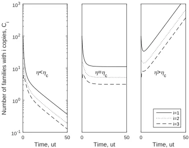
dt =kC , (2.17)
wherek is a constant. Clearlyk is an eigenvalue of the coefficient matrix of the ODE
system (2.13), and gives the longterm exponential growth rate; its corresponding
eigenvector gives the longterm distribution. While ηc corresponds to k = 0, the
condition η > ηc implies an increasing population and η < ηc implies a decreasing
population, where ηc is defined in (2.15).
We obtained the longterm growth rate, k, when k 6= 0 by finding the eigenvalue
con-vergence criteria outlined above, the eigenvalue was determined numerically with a
finite matrix size, N, and N was increased until the eigenvalue converged.
2-D Copy-Level Model
For the two dimensional model, Ri,j is the number of families with i copies in the
coding region, and j copies in the non-coding region. This can also be expressed as
dR1,0
dt =−(u1+w1 +v1)R1,0+ 2(v1+w1)R2,0
+(v2+w2)R1,1+
∞ X
i=0
∞ X
j=0
i+j6=0
(iv+ρη)Ri,j
dR0,1
dt =−(u2+w2+v2)R0,1+ 2(v2 +w2)R0,2+ (v1+w1)R1,1
+ ∞ X
i=0
∞ X
j=0
i+j6=0
(jv+ (1−ρ)η)Ri,j
dRi,0
dt =ρ(i−1)u1Ri−1,0−i(u1+w1+v1)Ri,0+ (i+ 1)(w1+v1)Ri+1,0
+(w2+v2)Ri,1, i≥2
dR0,j
dt = (1−ρ)(j −1)u2R0,j−1−j(u2+w2+v2)R0,j + (j+ 1)(w2+v2)R0,j+1
+(w1+v1)R1,j, j ≥2
dRi,j
dt =ρ((i−1)u1+ju2)Ri−1,j + (1−ρ)(iu1+ (j−1)u2)Ri,j−1
−(i(u1+w1 +v1) +j(u2+w2+v2))Ri,j
+(i+ 1)(w1+v1)Ri+1,j+ (j+ 1)(w2+v2)Ri,j+1, i, j ≥1 .
(2.18)
To estimate the longterm growth rate of the system, we integrate (2.18)
numeri-cally.
Genome-Level Model
We can similarly solve for an equilibrium solution to the genome-level model. When
condition (2.15) is not met, however, one of the parameters of the genome-level model,
µ, will not be constant. This HGT rate scales with the average number of families
per genome, ¯f. Intuitively, if the number of families with n copies is growing, for
all n, in a finite population of genomes, the mean number of families per genome
is likewise growing. Thus the equilibrium distribution derived for the genome-level
model is valid only when the copy-level model is at equilibrium.
Similar to our previous approach, the genome-level can be expressed as a system
as ODEs:
dFm
dt = ((m−1)p+µ)Fm−1−(m(p+q) +µ)Fm+ (m+ 1)qFm+1, m≥0 (2.19)
where Fm is the number of genomes containing m families of MGEs (and we define
F−1 = 0). Using the software package Maple, we are again able to find an analytic
solution in the case of dF¯
dt = 0, under the constraintp < q:
¯
Fm =
G
m!
p q
m Γ(m+ µ
p) Γ(µp)
1−p
q
µ/p
, (2.20)
where G is the number of genomes and Γ(x) is the gamma function.
Then, the proportion of genomes with m families, fm, is given by:
fm =
1
m!
p q
m Γ(m+µ
p) Γ(µp)
1− p
q
µ/p
. (2.21)
Unlike the copy-level model, we do not have to consider stationary solutions. In
this model there are no absorbing states, and the system will approach this equilibrium
as long as the condition p < q holds, and the parameters p, q and µ are constant. If
2.3
Results
It should be noted that it is the ratios of the parameters, rather than their actual
values, that affect the extinction probabilities and equilibrium state of the system.
We chose to normalize the 1-D copy-level and genome-level parameters by u and p
respectively, using notation ˆw=w/ufor example, or ˆq =q/p. For the 2-D copy-level
model, because the parameterηis shared by both regions of the genome, we normalize
by η, for example ˜w1 =w1/η. In previous work, best fit values for MPs were found
to be w/u = 0.9810, v/u = 0.0424, η/u = 0.0965, q/p = 1.24 and µ/p = 1.09 [88].
We will refer to these values from the promoter dataset as ˆwp, ˆvp, ˆηp, ˆqp and ˆµp,
respectively.
An important interaction occurs in this model between diversification and HGT.
Since HGT is not dependent on copy number, there is more HGT when there are
many families with few copies, as compared to few families with the same number of
total copies. Therefore, diversification acts indirectly to increase the amount of HGT.
2.3.1
Extinction Probability
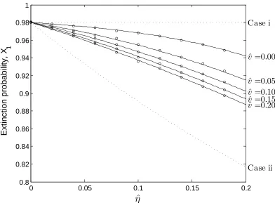
For the 1-D copy-level model, the extinction probability for a family of size 1, X1, is
illustrated in Figure 2.3. We find that increasing HGT, η, promotes survival, which
is reasonable since each HGT event adds a MGE copy. We also find, however, that
increasing diversification, ˆv, increases survival, but only in the presence of HGT. Since
a diversification event has no net effect on copy number, this is an interesting result
(see Section 2.4). Finally, we note that the parameters estimated for MPs, ˆwp, ˆvp and
ˆ
ηp, predict an extinction probability of X1 = 0.96.
In Figure 2.4, we examine the extinction probability for larger families, finding
that increasing family size,n, reduces the extinction probability as expected. In both
0 0.05 0.1 0.15 0.2 0.8
0.82 0.84 0.86 0.88 0.9 0.92 0.94 0.96 0.98 1
ˆ
η
Extinction probability, X
1
ˆ v =0.00
ˆ v =0.05
ˆ v =0.10
ˆ v =0.15
ˆ v =0.20 Case i
Case ii
Figure 2.3: Extinction probabilities of one member families,X1, for varying diversification
(ˆv) and horizontal gene transfer (ˆη) rates. The value of the deletion rate parameter is ˆ
respect to n. More generally, however, the solution to equation (2.3) does not obey
an exponential law as seen in the figure inset. In particular, for small families, the
extinction probability is lower than would be predicted by an exponential law.
0 1 2 3 4 5 6 7 8 9 10
0.2 0.3 0.4 0.5 0.6 0.7 0.8 0.9 1
Number of copies, n
Extinction Probability, X
n ˆ v =0.00 ˆ v =0.05 ˆ v =0.10 ˆ v =0.15 ˆ v =0.20 Case i Case ii 1 10 0.88 1
Figure 2.4: Extinction probabilities of nmember families,Xn, for varying diversification
rates (ˆv). Values used for HGT and deletion rates are ˆη = 0.1 and ˆw = 0.98 respectively. Results are shown for both the numerical solution (solid line), and Monte Carlo simulation (circles). Asymptotic cases are described in equations (2.4) and (2.5), and depicted as dotted lines. The inset shows the same data but with √n
Xn on the y-axis. With the exception of the asymptotic cases, the solutions do not obey an exponential law. All solutions are forn integer; lines are plotted continuously to guide the eye.
For the 2-D model, we compare the extinction probability of one member families
if they are initially present in the coding region to those in the non-coding region in
Figure 2.5. When ρ = 0, the extinction probability for one member families in the