Determining Real Permittivity from Fresnel Coefficients in GNSS-R

Progress In Electromagnetics Research M, Vol. 79, 159–166, 2019

Determining Real Permittivity from Fresnel Coefficients in GNSS-R

Patrizia Savi1, *, Silvano Bertoldo1, and Albert Milani2, 3

Abstract—Global Navigation Satellite System Reflectometry (GNSS-R) can be used to derive information about the composition or the properties of ground surfaces, by analyzing signals emitted by GNSS satellites and reflected from the ground. If the received power is measured with linearly polarized antennas, under the condition of smooth surface, the reflected signal is proportional to the modulus of the perpendicular and parallel polarization Fresnel coefficients, which depend on the incidence angle

θ, and on the dielectric constant ε of the soil. In general, ε is a complex number; for non-dispersive soils, the imaginary part of ε can be neglected, and a real value of ε is sought. We solve the real-valued problem explicitly giving formulas that can be used to determine the dielectric constant ε and we compare the analytical solution with experimental data in the case of sand soil.

1. INTRODUCTION

Global Navigation Satellite System Reflectometry (GNSS-R) is a technique for sensing the Earth surface, based on the principle of detecting GNSS signals reflected off the ground, and processing them to monitor its properties remotely (see [1]). This application is a key input in the areas of ocean observation (see e.g., [2]), ice (see e.g., [3, 4]) and land remote sensing (see e.g., [5–7]), altimetry (see e.g., [8, 9]), climate modeling and weather prediction [10]. The passive bi-static radar configuration used in this technique requires no transmitters except GNSS satellites, thus enabling the system to be light and compact (see e.g., [11–14]). The Signal to Noise (SNR) data recorded by GNSS receivers are related to the direct signals and those reflected by the ground. Under the assumption that the surface be flat, and considering a receiving antenna either vertically or horizontally polarized, the SNR is related to the Fresnel reflection coefficients for vertical and horizontal polarization, which are functions of the relative permittivity of the soil and of the incident angle [15]. The relative permittivity of the soil is generally obtained by solving the Fresnel coefficient equations numerically; then, the soil moisture can be obtained by applying several well established models (see for example the semi-empirical models of [16, 17]). These models may be useful for the monitoring of a field of known characteristics in terms of sand, clay percentage, etc. In more general cases, i.e., for non-flat surfaces, more powerful techniques of inverse scattering should be used [18].

2. STATEMENT OF THE PROBLEM

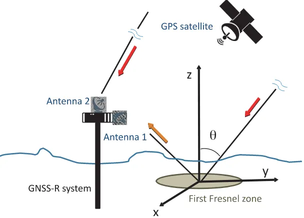
The total electromagnetic field received by the down-looking antenna is the sum of various signals, scattered by the Earth’s surface (see Fig. 1). These are essentially of two kinds: coherent and incoherent [19]. If the surface is approximately smooth, the non-coherent component is negligible, and the total power received by the antenna can be approximated by the coherent part only [5].

Received 7 December 2018, Accepted 11 March 2019, Scheduled 15 March 2019

* Corresponding author: Patrizia Savi (patrizia.savi@polito.it).

1 _{Department of Electronics and Telecommunications, Politecnico di Torino, Corso Duca degli Abruzzi 24, Torino 10129, Italy.} 2 _{Department of Mathematics, Politecnico di Torino, Corso Duca degli Abruzzi 24, Torino 10129, Italy.} 3 _{Botswana International}

Figure 1. GNSS reflectometry geometry.

The coherent component in the GPS bistatic radar is given by

Ppol, coh =Rpol PtGtGrλ 2

(4π)2₍r1₊r2₎2, (1)

where the productP_tG_t is the Equivalent Isotropic Radiated Power (EIRP) of the transmitted signal;

Gr is the receiver antenna gain; λis the wavelength (λ= 19.042 cm for GPS L1 signal);r1 and r2 are, respectively, the distance between the receiver and the specular point, and that between the specular point and satellite; R_p is the power reflectivity of the reflecting surface at a specified polarization (pol). For smooth surfaces, the reflectivity can be approximated by

Rpol =|Γpol|2, (2)

where Γ_pol is the Fresnel reflection coefficient. In the case of perpendicular (or horizontal, or TE) polarization and parallel (or vertical, or TM) polarization, the corresponding Fresnel reflection coefficients can be written, respectively, as:

Γ_n= cosθ−

ε−sin2θ cosθ+ε−sin2θ,

Γ_p= εcosθ−

ε−sin2θ

εcosθ+ε−sin2θ.

(3)

Progress In Electromagnetics Research M, Vol. 79, 2019 161

3. THE FRESNEL INVERSE PROBLEM

We look for real solutions ε >1 (to signify that the medium is denser than air) to either the equation

cosθ−ε−sin2θ cosθ+ε−sin2θ

=|Γn|=:γn, (4)

or

ε

cosθ−ε−sin2θ

εcosθ+ε−sin2θ

=|Γp|=:γp, (5)

with θ ∈ [0,π₂[ and, correspondingly, 0 < γ_p ≤ γ_n < 1 (these conditions are necessarily satisfied if Eqs. (4) and (5) do have a common solution). Then, Equation (4) has a unique solutionε_n>1, given by

εn= 1 +4γncos 2_θ

(1−γ_n)2. (6)

This solution is constant under certain compatibility conditions between γ_n and θ similar to Eq. (15), in the sense that εis independent of the particular angleθ at which the values ofγ_n is measured. The determination of an explicit, constant solution of Eq. (5) is more complicated. We assume that there is

θB ∈]π₄,π₂[, corresponding to which γ_p = 0 (θ_B is the Brewster angle; this too is a necessary condition for solvability). We define

λp := 1 +₁₋γ_γp

p ≥1, (7)

and note that λ_p = 1 only whenγ_p = 0. We define further

μp :=

⎧ ⎨ ⎩

λp if 0≤θ≤θ_B, 1

λp if θB≤θ < π

2

(8)

(recall that λ_p = _λ1

p = 1 at θB), and

θ1 := ⎧ ⎪ ⎨ ⎪ ⎩ π

2 if tan

2_θ B ≥2,

arcsin

1 √

2tanθB if tan

2_θ B <2.

(9)

Then, Equation (5) has a solutionε_p>1, given by

εp = μp 2 cos2_θ

μp+ sgn(θ1−θ)

μ2

p−sin2(2θ) . (10)

This solution is obtained by patching together three different solutions ε0

p, defined on all of [0,π2[, and ε1

p,ε2p, defined only in [θB,π2[, as long asλpsin(2θ) ≤1 in this interval. The three solutions are given

by:

ε0

p = λ

2 p 2 cos2_θ

1 +

1−sin

2_(2θ)

λ2 p

, (11)

ε1

p = _2λ2 1 pcos2θ

1 +

1−λ2

psin2(2θ) , (12)

ε2

p = _2λ2 1 pcos2θ

1−

1−λ2

psin2(2θ) . (13)

In principle, these solutions depend onθ, and satisfy the conditions:

ε0

Figure 2. Solution of (5). On [π₄, θ_B], ε = tan2θ_B = ε0_p; on [θ_B, θ1], ε = tan2θ_B = ε1_p; on [θ1,π₂[,

ε= tan2θ_B=ε2_p.

We find that the constant solution to the Fresnel formulas is given byε_p = tan2θ_B (as is well known); however,ε0_pcan be constant only ifθvaries between π₄ andθ_B, because, afterθ_B,ε0_p >tan2θ_B2. Likewise,

ε1

p can be constant only whenθvaries betweenθB andθ1, because, afterθ1,ε1p >2 sin2θ >tan2θB. On the other hand,ε2_p can be constant forθbetweenθ1 and π₂, because tan2θ_B< ε2_p <2 sin2θ(see Fig. 2).

The solutions ε_n and ε_p coincide on all of [0,π₂[ if and only if the compatibility condition:

λ2

ncos2θ+ sin2θ=λnμp (15)

holds in [0,π₂[, where, as in Eq. (7),

λn:= 1 +₁₋γ_γn

n >1, (16)

together with the additional conditionsγ_p≤γ_n2, if θ_B ≤θ≤θ1, or γ_n2 ≤γ_p, if θ1 ≤θ < π₂. In this case, the common solution ε_n=ε_p =:ε_c is given by

εc =λ_nμ_p, (17)

and ε_c is constant on [0,π₂[; in fact, as mentioned above,

εc = tan2θB. (18)

Progress In Electromagnetics Research M, Vol. 79, 2019 163

which case ε= 2 sin2θ1 = 2λ2_n/(1 +λ_n2). More precisely, the case θ= π₄ and γ_n2 =γ_p is exceptional, in that Equations (4) and (5) are identities inε; that is,any ε∈IR (in fact, anyε∈Cl ) is a solution.

The reflected GPS signals are predominantly LH [5], especially for satellites with high elevation (angles greater than 60◦). Using the Subscript LR to represent the scattering when a satellite incident signal (right-hand polarized) is scattered by the surface and inverts the polarization to the left-hand, the reflection coefficient, Γ_LR, can be written as a linear combination of vertical and horizontal polarization [15]:

Γ_LR = 1

2(Γn−Γp) (19)

Note that:

γn = 1₂(|Γn−Γp|+|Γn+ Γp|) (20)

γp = 1₂||Γn−Γp| − |Γn+ Γp|| (21) Ifθ= 0◦, then Γ_n=−Γ_p, therefore:

γn = 1₂|Γn−Γp|=|ΓLR| (22)

γp = γn (23)

The values of signal to noise ratio (SNR) can be obtained from the GNSS-R measurements considering various satellites with different elevation angles. Considering the satellites with high elevation angles (i.e., θ∼0), the SNR values the amplitude of the reflection coefficient |Γ_LR|can be obtained and the value of permittivity evaluated from 10.

4. RESULTS

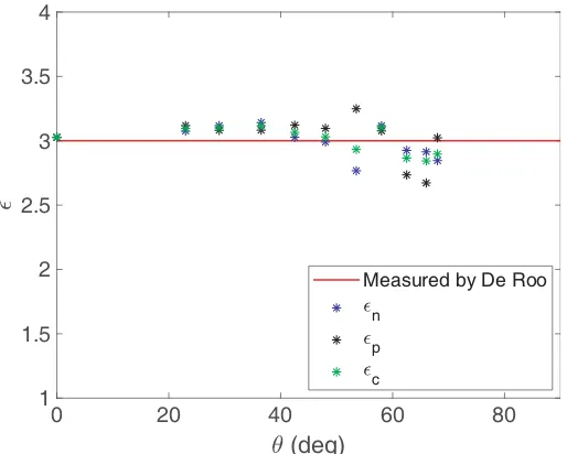
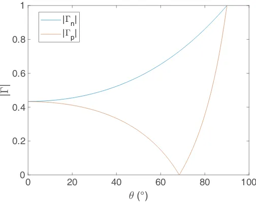
As a first example, in Fig. 3 we consider the measurements of|Γ_n|and|Γ_p|reported in [18] for a medium composed of sand, for whichε= 3 +σj, with|σ| ≤0.05. We compute the values ofε_n andε_p predicted by Eqs. (6) and (10), as well as the common valueε_c =λ_nλ_p.

We find that these values match the approximate value ε≈ 3 with error not exceeding 1%. The measurements of |Γ_p| point to the evidence of a possible Brewster angle at approximately θ_B = 60◦ (which would be the exact value for ε= 3). The relative error is given by e_c := 1₃|ε_c−3|(see Fig. 4).

0 20 40 60 80

(deg) 0

0.2 0.4 0.6 0.8 1

|

|

| |

n theoretical

| |

p theoretical

| |

n measured by De Roo

| |

p measured by De Roo

0 20 40 60 80 (deg)

1 1.5 2 2.5 3 3.5 4

Measured by De Roo

n

p

c

Figure 4. Relative error.

As a second example, we consider some GNSS-R measurements carried out in a controlled environment located in Grugliasco, Torino (450358.5N, 73533.8E). In this location, a wide field of known characteristics (mainly 50% sand) belonging to the Interuniversity Department of Regional and Urban Studies and Planning (DIST), Politecnico di Torino, is available. The composition of the terrain is reported in Table 1. In this campaign, the direct GPS signals were measured using a right-hand circular polarized (RHCP) antenna, while the reflected signals were measured with a left-hand circular polarized (LHCP) antenna. The complete description of the setup can be found in [21]. In addition to the GNSS-R measurements, Time-Domain Reflectometry (TDR) measurements were carried out to be used as reference. An average value of about 6.4 was obtained for the permittivity. In Fig. 5, the magnitude of the two reflection coefficients is reported for = 6.4. In particular, for a permittivity value equal to 6.4, for an elevation angle higher than 80◦ (corresponding to an incidence angle θ less than 20◦), the difference between|Γ_n|and|Γ_n|is less than 0.043. In this case, the real permittivity can be obtained by using formula (10) for |Γ_p|.

The results of the GNSS measurements and the computation of the permittivity values are reported in Table 2. Only satellite PRN 9 is considered because of its elevation. It can be observed that the values with an elevation angle greater than 80◦are close to the results obtained with the TDR technique.

Table 1. Composition of the soil for the Grugliasco experiment.

Coarse sand (%) Fine sand (%) Very Fine sand (%)

115.5 50.1 16.1

Coarse silt (%) Fine silt (%) Clay (%) Organic matter(%)

5.3 8.2 4.8 1.4

Table 2. Computation of the permittivity values from the measurements.

Elevation (deg) θ (deg) SNR (dB) |Γ_LR|

82.4 7.6 11 0.195 6.57

Progress In Electromagnetics Research M, Vol. 79, 2019 165

0 20 40 60 80 100

(°) 0

0.2 0.4 0.6 0.8 1

|

|

| _n| | _p|

Figure 5. Amplitude of reflection coefficients for= 6.4.

5. CONCLUSIONS

In GNSS-R for soil moisture applications, one essentially needs to determine the permittivity ε of the soil from the Fresnel coefficients. For non-dispersive soil,ε can be assumed real. In the literature, εis mostly found numerically. In fact, Equations (4) and (5) can be explicitly solved. We determine real solutions withε >1, for all angles θ∈[0,π₂[ and all measurements γ_n,γ_p ∈]0,1[, with γ_p ≤γ_n, which satisfy the compatibility conditions (15).

Our results suggest two possible strategies to determine the solution. The first hinges on being able to find a valueγ_p≈0 at a particular position ˜θ; then, ˜θis an approximation of the Brewster angle, and the approximate solution is simplyε≈tan2θ˜, as per Eq. (18). Otherwise, one can take any angle

θ in [0,π₄[, and verify that the corresponding measurements of γ_n and γ_p satisfy condition (15). If so, the solution is ε=λ_nλ_p, as per Eq. (17).

ACKNOWLEDGMENT

The third author acknowledges the support and the kind hospitality of the Department of Mathematics of Politecnico di Torino during his time as visiting professor there.

REFERENCES

1. Jin, S., E. Cardellach, and F. Xie, GNSS Remote Sensing: Theory, Methods and Applications, Springer, 2014.

2. Zavorotny, V. U. and A. G. Voronovich, “Scattering of GPS signals from the ocean with wind remote sensing application,”IEEE Transactions on Geoscience and Remote Sensing, Vol. 38, No. 2, 951–964, March 2000.

3. Wiehl, M., B. Legr´esy, and R. Dietrich, “Potential of reflected GNSS signals for ice sheeet remote sensing,”Progress In Electromagnetics Research, Vol. 40, 177–205, 2003.

4. Alonso-Arroyo, A., V. U. Zavorotny, and A. Camps, “Sea ice detection using U.K. TDS-1 GNSS-R data,” IEEE Transactions on Geoscience and Remote Sensing, Vol. 55, No. 9, 4989–5001, 2017. 5. Masters, D., A. Penina, and S. Katzberg, “Initial results of land-reflected GPS bistatic radar

6. Ban, W., K. Yu, and X. Zhang, “GEO-satellite-based reflectometry for soil moisture estimation: Signal modeling and algorithm development,” IEEE Transactions on Geoscience and Remote Sensing, Vol. 56, No. 3, 1829–1838, 2018.

7. Pierdicca, N., A. Mollfulleda, F. Costantini, L. Guerriero, L. Dente, S. Paloscia, E. Santi, and M. Zribi, “Spaceborne GNSS reflectometry data for land applications: An analysis of techdemosat data,” International Geoscience and Remote Sensing Symposium (IGARSS), 3343–3346, Valencia, Spain, July 22–27, 2018.

8. Li, W., A. Rius, F. Fabra, E. Cardellach, S. Rib´o, and M. Mart´ın-Neira, “Revisiting the GNSS-R waveform statistics and its impact on altimetric retrievals,”IEEE Transactions on Geoscience and Remote Sensing, Vol. 56, No. 5, 2854–2871, 2018.

9. Mashburn, J., P. Axelrad, S. T. Lowe, and K. M. Larson, “Global ocean altimetry with GNSS reflections from TechDemoSat-1,”IEEE Transactions on Geoscience and Remote Sensing, Vol. 56, No. 7, 4088–4097, July 2018.

10. Cardellach, E., et al., “GNSS Transpolar Earth Reflectometry exploriNg System (G-TERN): Mis-sion concept,”IEEE ACCESS, Vol. 6, 13980–14018, 2018, DOI: 10.1109/ACCESS.2018.2814072. 11. Katzberg, S., O. Torres, M. Grant, and D. Masters, “Utilizing calibrated GPS reflected signals

to estimate soil reflectivity and dielectric constant: Results from SMEX02,” Remote Sensing of Environment, Vol. 100, 17–28, 2005.

12. Egido, A., M. Caparrini, G. Ruffini, S. Paloscia, E. Santi, L. Guerriero, N. Pierdicca, and N. Floury, “Global navigation satellite systems reflectometry as a remote sensing tool for agriculture,”Remote Sensing, Vol. 4, 2356–2372, 2012.

13. Yu, K., C. Rizos, D. Burrage, A. G. Dempster, K. Zhang, and M. Markgraf, “An overview of GNSS remote sensing,” EURASIP Journal on Advances in Signal Processing, 2014–2134, 2014.

14. Pei, Y., R. Notarpietro, P. Savi, and F. Dovis, “A fully software GNSS-R receiver for soil monitoring,”International Journal of Remote Sensing, Vol. 35, No. 6, 2378–2391, 2014.

15. Stutzman, W. L., Polarization in Electromagnetic Systems, Artech House, 1993.

16. Wang, J. and T. Schmugge, “An empirical model for the complex dielectric permittivity of soils as a function of water content,” IEEE Transactions on Geoscience and Remote Sensing, Vol. 18, No. 4, 288–295, 1980.

17. Hallikainen, A. and F. Ulaby, “Microwave dielectric behavior of wet soil — Part 1: Empirical models and experimental observations,” IEEE Transactions on Geoscience and Remote Sensing, Vol. 23, No. 1, 25–34, Jan. 1985.

18. Roo, R. D. and F. Ulaby, “Bistatic specular scattering from rough dielectric surfaces,” IEEE Transactions on Antennas and Propagation, Vol. 42, No. 2, 220–231, 1994.

19. Pierdicca, N., L. Guerriero, M. Brogioni, and A. Egido, “On the coherent and non coherent components of bare and vegetated terrain bistatic scattering: Modelling the GNSS-R signal over land,” Proc. IEEE Int. Geosci. Remote Sens. Symp., 3407–3410, Munich, Germany, July 22–27, 2012.

20. Savi, P. and A. Milani, “Real-valued solutions to an inverse Fresnel problem in GNSS-R,” Inernational Geoscience and Remote Sensing Symposium (IGARSS2018), 3327–3330, Valencia, Spain, July 22–27, 2018.