Weather Levels Based on Improved Upstream Meshless Method”
by Bing Gao, Fan Yang, Haizhou Qian, Min Liu, Chunli Li, and Chao Liu
in Progress In Electromagnetics Research M, Vol. 74, 147–157, 2018
Bing Gao1, *, Fan Yang1, Zhouhai Qian2, Min Liu2, Chunli Li3, and Chao Liu4
The name of the third author in this paper should be Zhouhai Qian.
Received 30 November 2018, Added 5 December 2018
1 State Key Laboratory of Power Transmission Equipment & System Security and New Technology, School of Electrical Engineering,
Chongqing University, Chongqing 400044, China. 2State Grid Zhejiang Electric Power Corporation Research Institute, Hangz Zhou,
Zhejiang 310000, China. 3Chongqing Three Gorges University, Chongqing 404000, China.4College of Power Engineering, Chongqing
The Ionized Field Calculation under Different Haze Weather Levels
Based on Improved Upstream Meshless Method
Bing Gao1, *, Fan Yang1, Haizhou Qian2, Min Liu2, Chunli Li3, and Chao Liu4
Abstract—The haze-prone areas are usually places with limited transmission line corridors and large power loads. The performance of transmission lines is under threat of haze. The haze particulates around the transmission lines would be charged and affect the electric field near high voltage direct current (HVDC) transmission lines. According to the influence mechanism of haze on ionized field, the electric performance of HVDC transmission lines under haze weather is discussed. In the paper, an improved meshless local Petrov-Galerkin method (MLPG) is proposed to investigate the distribution of ionized electric field, and example of an actual transmission line is studied to verify the validation of the proposed method at first. It is proved that the proposed method agrees well with the measurements. Then the ionized field distribution under different haze weather levels, as well as influenced factor, is discussed. Results indicate that the ionized electric field and ion current density on the ground would increase under haze weather, but with similar trends to good weather condition. Meanwhile, the haze weather levels have greater influence on the ionized electric field than ion current density, where the increase of corona and space charge are the main reasons.
1. INTRODUCTION
The HVDC transmission lines are widely constructed in China to transmit the power energy over long distance [1].
The ionized electric field and ion current density at the ground level due to the corona have to be analyzed in advance to obtain an optimal design and avoid flashover [2]. However, the performance of transmission lines is under threat of haze, because the haze-prone areas are usually the places with limited transmission line corridors and large power loads. The haze particulates in the air would be charged, and these particulates can be absorbed on the conductor surface, leading to change of onset electric field and space charge density [3, 4]. Therefore, there is no doubt that the haze weather conditions would strengthen the ionized field and make the ionized field calculation more complex [5]. It is important to investigate the distribution of ionized electric field and ion current density in consideration of different haze weather levels and temperature.
Researches on impact of environment situations are mainly focused on wind speed, as well as the corresponding calculation model. Meanwhile, it has been proved that other weather conditions have also significant influence on ionized field. Comber and Johnson had measured the ionized field under normal weather and rainy weather, which indicates that both the corona degree and ionized field increased obviously due to the raindrop absorption on conductor surface [6]. Johnson had pointed out that the ionized field and ion current density of ground level would vary with seasons, in addition, the minimum
Received 12 March 2018, Accepted 16 August 2018, Scheduled 14 October 2018 * Corresponding author: Bing Gao ([email protected]).
1 State Key Laboratory of Power Transmission Equipment & System Security and New Technology, School of Electrical Engineering,
and maximum value happen in winter and September, respectively [7]. Fan et al. investigated the impact of environment temperature, and it was proved that the ionized field becomes stronger if the temperature is higher [8]. Lu et al. had pointed out that the ionized electric field and ion current density would increase with rainy weather, which should be taken into accounted in transmission lines design [9]. Zhao and Zhang studied the ionized electric field of fog conditions, and it was found that the fog would be absorbed on the conductor surface and enhance the corona degree [10].
However, most researches rarely focus on the influence of haze weather, which would enhance the ionized field. In addition, to calculate the ionized field, many methods have been used to solve the coupling equations; however, the meshless methods do not need any connectivity structure among nodes, avoiding the mesh generation problem [11]. Therefore, this paper proposes an improved MLPG method to study the ionized electric field under different haze weather levels.
The paper begins with the influenced mechanism of haze weather, as well as the governing equation of ionized field in the presence of haze in Section 2. In Section 3, the detailed information of the improved MLPG upstream method is introduced to determine the ionized field. After the verification of the algorithm, the distribution of ionized field at ground level under different haze weather levels is investigated in Section 4. The influenced factors are also discussed to show the influence of haze levels in Section 5. This paper ends with conclusions and discussions in Section 6.
2. METHOD BASIC
2.1. The Influenced Mechanism of Haze Weather
It is well known that the haze weather often happens in China, as it produces large amount of haze particulates, which are charged around high voltage transmission lines and enhance the ionized electric field. Therefore, it is necessary to investigate the influence of haze weather for structure design and operation maintenance. The main components of haze are PM 2.5, PM 10 and fog. The influence of haze weather on ionized field of HVDC lines can be divided into ion mobility, space charged ion density and conductor surface roughness factor.
Since the charge of haze particulates is mainly determined by their diameters, the calculated diameters of PM 2.5, PM 10 and fog are chosen as 1.3µm, 5.6µm and 3.2µm, respectively. Therefore, only the influence of electrical charge is considered, and the corresponding charge of haze particulates can be expressed as:
qs= 4πε0
3εr
εr+ 2a
2E
0 (1)
where qs is the saturation charge, ε0 the permittivity of vacuum, 8.854×10⁻¹²F/m, a the radius of
particulates, and E0 the applied electric field, which is 10 kV/cm in the paper.
On the other hand, the saturated charged particulates would affect the ion mobilityK, which can be described as:
K K=
m
a
ma+mh+mp (2)
where K is the ion mobility of good weather, ma the density of dry air, mh the water vapor content, which is 23 g/m3, andmp the haze particulates content.
Therefore, the ion mobility can be derived as equation on basis of the concentration of different haze weather levels.
K
+/−≈(1−0.015A)K+/− (3)
whereA is the air pollution level, of which value varies 1∼6.
Due to the absorption effect of haze particulates, the surface roughness coefficient of transmission lines would change. Reference [12] indicates that the surface roughness coefficient is 0.4 in rainy weather, while the corresponding value is 0.44 for fog weather condition. Because the surface of transmission line is affected by both fog and suspension particulates, leading to rougher situation than fog case, while it is smoother than rainy condition, the roughness coefficient is chosen as 0.42. Consequently, the onset electric field for different weather conditions can be written as:
Eon = m
wherem is the surface roughness coefficient, which is 0.42 in the paper,Eon the ionized electric field of haze weather condition, Eon the onset electric field of good weather, and the corresponding roughness coefficientm is chosen as 0.47.
2.2. Basic Equations of Ionized Field for Haze Weather
To simplify the problem of haze weather condition, the following assumptions are made [13].
1) The motilities K+ and K− of positive and negative ions are constant respectively, independent of
local electric field strength. The particles are evenly distributed in the space and regarded as static. 2) The diffusion of ions is negligible. Fog and haze are only charged by the field, and the charge quantity is saturated. Besides, the local electric field distortion caused by charged haze particulates is also ignored.
3) The interaction of the particles is neglected, while the fog and haze will not convert to each other. Based on the above assumptions, considering the impact of fog and haze, the equations used for bipolar field are as follows:
∇2ϕ = (ρ
−−ρ+)/ε (5)
Es = −∇ϕ (6)
j+ = ρe+(K+ Es+w) (7)
j− = ρe−(K+ Es−w) (8)
∇ ·J+ = −Rρ+ρ−/e (9)
∇ ·J− = Rρ+ρ−/e (10)
where,
ρ+/−=ρe+/−+ρf+/−+ρp1+/−+ρp2+/− (11)
where the subscripts + and −are only for positive charges and negative charges; ρ is the total space charge, C·m−3;ϕis the potential, V;Jis the current density, A·m−2;wis the velocity vector, m·s−1;
R is the ion recombination coefficient, m3·s−1;eis the charge of the electron, 1.602×10⁻¹⁹C; ρe is the space ionized charge density, C·m−3;ρp1 is charge density of PM 2.5, C·m−3;ρp2 is the space charge
densities of PM 10, C·m−3;ρf is the space charge densities of droplet, C·m−3.
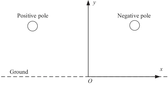
The studied bipolar pole DC transmission line is illustrated in Fig. 1, and the boundary conditions are listed as follows.
O
Ground x
y
Positive pole Negative pole
Figure 1. The model of bipolar DC transmission line.
On the conductor surface
ϕ=±U (12)
The potential on the ground plane is zero
ϕ= 0 (13)
In the programming, calculation can only be applied in a limited region; therefore, an artificial boundary is placed far enough from the conductors, where the charge density should be small enough to be neglected.
The potential on the artificial boundary
ϕ=ϕ0 (14)
whereϕ0 is the potential at the artificial boundary without space charge.
According to the Kaptzov’s assumption, on the transmission line surface, the magnitude of electric field strength at the coronation conductors remains at the onset value.
Es=Eon± (15)
whereEs is the surface electric filed on the positive and negative poles.
3. THE IMPROVED UPSTREAM MLPG FOR IONIZED FIELD CALCULATION
3.1. Improved MLPG Method
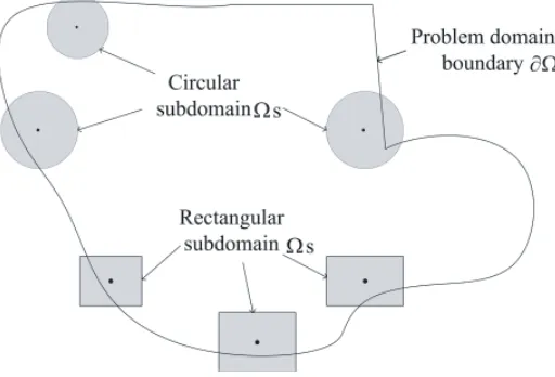
Since the meshless method does not require elements or meshes either to solve the distribution of electric field in the calculation of shape function or the interpolation process, this method can solve the above equations efficiently. Therefore, the MLPG meshless method, which is based on the local symmetric weak form, is adopted to solve the Poisson’s equations. During the traditional MLPG method, as shown in Fig. 2, the same local subdomain is chosen to deal with the integral problems. However, in the boundary integrations of regular MLPG method, the intersections between local sub-domains and global boundary are required. It can be very hard to determine the intersections between the local sub-domains and the global boundary for problems with irregular boundary.
Figure 2. The intersection between the local sub-domain Ωs and the global boundary.
Adjusting the local sub-domain Ωs
near boundary
Boundary domain ∂Ω
Figure 3. The local sub-domain Ωs near the global boundary have been adjusted to avoid crossing the standard limitation boundary.
3.2. Solution of Charge Density Using Upstream Meshless Method
The upstream MLPG derives from the upstream FEM method has been developed by shifting the local subdomain opposite to the streamline direction, as shown in Fig. 4.
jj i
k
m l n Normal Local
Sub-domain Upstream Local
Sub-domain
Figure 4. Meshless method upstream scheme.
The nodes includingm,jand k, located in the upstream local subdomain, are selected to calculate the charge density of nodei. The proposed method can capture the information from upstream, and in practice, it is found that three to six upstream nodes are good enough for the precise calculation [14].
According to the basic Equations (7)–(10), we can have
k+
ε0ρ 2 ++
Rρ−
e − k+ρ−
ε0
ρ++∇ρ+·v+ = 0 (16)
k− ε0ρ
2
−+
Rρ
+
e − k−ρ+
ε0
ρ−+∇ρ−·v− = 0 (17)
where v+ = K+Es and v− = K−Es are the migration velocity of the positive and negative ions,
respectively.
In the MLPG meshless method, the charge density of the local subdomain can be obtained as follows:
ρ(x) =
n
I
ΦI(x)ρI (18)
Inserting Equation (18) into Equations (16)–(17), will result in:
k+/−
ε0 ρ 2 +/−+
Rρ
−/+
e −
k+/−ρ−/+
ε0 ρ+/− + n I
ΦI,x(x)ρI+/−·vix+/−+ ΦI,y(x)ρI+/−·viy+/−
= 0 (19)
After simplification,
A+/−ρ2+/−+B+/−ρ+/−+C+/− = 0 (20)
where
A+/− =
K+/−
ε0
(21)
B+/− =
R/e−K+/−/ε0
ρ−/++Φi,x(x)vix+/−+ Φi,y(x)viy+/− (22)
C+/− = n
I(I=i)
ΦI,x(x)ρI+/−vix+/−+ ΦI,y(x)ρI+/−·viy+/− (23)
where ΦI,x and ΦI,y denote ∂(ΦI)/∂x and∂(ΦI)/∂y, respectively.
By solving the above total set of equations in the whole region, the charge density at every node can be obtained.
Since the space charge and electric field are coupled, we chose to apply an iterative algorithm to solve the system of Eqs. (2)–(7). The criterions of ionized electric filed calculation are listed as follows:
δρ = |ρn−ρn−1|/ρn−1 (24)
δE = |Emax−Eon|/Eon (25)
where ρn and ρn−1 are the nth and n−1th calculated surface charge densities of conductor; Emax is
the maximum electric field of conductor surface. During the iterative calculation process, the surface density of conductor has to be updated, which can be expressed as:
ρn=ρn−1[1 +μ(Emax−Eon)/(Emax+Eon)] (26)
where ρn and ρn−1 are the nth and n−1th calculated surface charge densities of conductor; μis the
correctness coefficient, which is 0.6.
3.3. Verification of the Algorithm
To verify the validation of the proposed method in ionized field calculation, an example of high voltage transmission line is calculated using the improved MLPG method and finite element method (FEM). The comparisons between FEM results in [13], MLPG results and measured data of electric field are shown in Figs. 5–6. It can be found that the proposed MLPG method deals well with ionized field problem, and the MLPG has smaller difference with experimental results than FEM method. Besides, the improved MLPG results have good coincidence with measured data.
In addition, another example of ±400 kV bipolar DC transmission line is also investigated on basis of the measured ionized field results given by Johnson [7]. The line distance is 12.2 m, and the equivalent radius of conductor is 45.7 cm. The studied heights of transmission lines are 10.7 m and 15.2 m, respectively. The ion mobility of positive ions and negative ions areK+ = 1.5×10⁻⁴m2·(Vs)−1
and K− = 1.7×10⁻⁴m2 ·(Vs)−1, respectively. The comparisons between the measured results in [7]
and the MLPG results of ionized electric field at ground level are shown in Fig. 7.
(a) (b)
Figure 5. Comparison between measured, FEM MLPG method of electric field. (a) Wind speed: 0 m/s. (b) Wind speed: 8 m/s.
(a) (b)
Figure 6. Comparison between the measured, FEM and Meshless Method of ion current at ground-level. (a) Wind speed: 0 m/s. (b) Wind speed: 8 m/s.
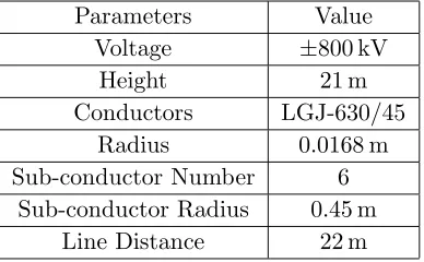
Table 1. The transmission line parameters.
Parameters Value Voltage ±800 kV
Height 21 m Conductors LGJ-630/45
Radius 0.0168 m Sub-conductor Number 6
Figure 7. Comparison of calculation results and experimental data of±400 kV DC transmission line.
4. IONIZED FILED UNDER DIFFERENT HAZE WEATHER
Then, an actual±800 kV HVDC transmission line is chosen, and the ionized electric field of haze weather is studied. The detailed parameters of transmission line are given in Table 1.
The particulates distribution of different haze weather levels are defined as in Table 2 on basis of the air quality controlled standard. It is assumed that light fog accompanies with heavy pollution level, in which the fog concentration is 100 drop/m3. Besides, medium fog occurs in serious pollution weather situation, with concentration about 200 drop/m3 [14]. Moreover, the density of haze particulates and suspended fog is 1 g/cm3 [15]. The permittivities of fog and haze particles are 38 and 8, respectively. The calculated diameters of PM 2.5, PM 10 and fog are 1.3µm, 5.6µm and 3.2µm, respectively. Consequently, combined with the proposed method described in Section 2, the ionized electric field can be achieved.
Table 2. Particles distribution under different pollution degree.
Types PM 2.5 (µg/m3) PM 10 (µg/m3) Droplet (drop/m3)
Good weather 20 40 0
Medium Pollution 180 250 100 Heavy Pollution 310 430 200 Serious pollution 510 1200 200
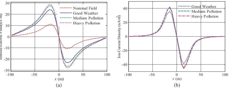
The ionized electric field and ion current density of different haze weather levels are shown in Fig. 8, in which the good weather case is also compared. One can see that all the ionized electric field and ion current density have similar variation tendency. The maximum and minimum values are close to the projection position of bipolar transmission line. Meanwhile, the absolute value increases with haze weather levels. For medium and heavy pollution cases, the increments of ionized electric field are 3.5 kV/m and 4.7 kV/m, increased by 14.5% and 19.5%, respectively. However, it is obvious that the haze weather has greater influence on the ionized electric field, compared to ion current density. The difference of ion current density among different haze weather levels is little, with increase about 5.58 nA/m2. The maximum ion current density of all cases is 41.42 nA/m2, which is smaller than the permitted value 100 nA/m2.
As stated that the ionized electric field increases with haze levels. However, the haze weather becomes worse in September, and the PM 2.5 would be over 500µg/m3, even exceeds 800µg/m3.
-100 -50 0 50 100 -30 -20 -10 0 10 20 30
x (m)
Io n iz e d E lec tr ic F iel d (kV /m ) Nominal Field Good Weather Medium Pollution Heavy Pollution
-100 -50 0 50 100
-40 -20 0 20 40 x(m) Io n C u rren t D ensity (nA /m 2 ) Good Weather Medium Pollution Heavy P ollution
(a) (b)
Figure 8. The distribution of ground level ionized field in the presence of very serious pollution haze. (a) Total electric field. (b) Ion current density.
are listed in Table 2, and the calculated ionized electric field and ion current density are given in Table 3. It can be seen that the maximum ionized electric field increases by about 23.49%, achieving about 29.8 kV/m, which is close to the permitted standard value 30 kV/m. Meanwhile, the maximum value of ion current density is 41.82 nA/m2, which increases by about 16.69% compared to good weather condition. On the other hand, the increased value is not proportional to the pollution level, and the main reason is that the free space charge would be captured by haze particulates, leading to decrease of space free charge and increase of charged haze particulates. These charged particulates move slower than space free charge, thereby the ion current density changes little for different pollution levels.
Table 3. The maximum value and growth rate of ground level total electric field and ion current density in presence of different haze.
Pollution Levels Concentration of PM 2.5 Emax Increment Jmax Increment
Good Weather 20µg/m3 24.13 0 35.84 0 Medium Pollution 180µg/m3 27.64 13.3% 41.42 15.57%
Heavy Pollution 310µg/m3 28.8 19.1% 41.73 16.43% Serious Pollution 510µg/m3 29.8 22.8% 41.82 16.69%
Table 4. The maximum value and growth rate of ground level total electric field and ion current density in presence of haze which only for consideration of one affecting factor.
Factors Emax Increment Jmax Increment
5. INFLUENCE CAUSED BY HUMIDITY AND TEMPERATURE
To investigate the influenced mechanism of haze weather on ionized electric field further, the influence degree of each impact factor is discussed, as listed in Table 4. It is obvious that the increased space charge density caused by haze weather would reduce the ion current density and promote the ionized electric field. While the corona degree enhances both the ionized electric field and ion current density, for example, the corresponding increment values are 18.58% and 20.06%, respectively. Consequently, the increase of ionized electric field and ion current density are mainly contributed by space charge density and corona degree, while the ion mobility has little effect on the ionized field and even will restrict the increase of ionized field. In conclusion, due to the strong coupling effect between space charge density and ionized electric field, the influence of haze weather on space charge density, ion mobility and onset electric field should be taken into account together.
It is known that the ambient environment has great influence on the ionized field, and the influence of humidity has been counted through fog toughness coefficient in ionized field calculation model. The ionized field of the HVDC transmission lines with different temperatures has been discussed in this section. Fig. 9 shows the variation of ionized electric field and ion current density under different temperature cases.
(a) (b)
Figure 9. The distribution of ground level ionized field in the presence of serious pollution haze with different temperature. (a) Ionized electric field. (b) Ion current density.
It can be seen that the ionized electric field and ion current density increases with temperature. When the ambient temperature increases to 303 K, the ionized electric field and ion current density increase by 1.7 kV and 7.9 nA/m2, achieving 6.1% and 19.6%, respectively. The main reason is that the conductor core temperature increases with the rising of ambient temperature, leading to decreasing of electric field and promoting of the corona degree.
6. CONCLUSION
The ionized electric field of haze weather is investigated on basis of the improved MLPG method, in which the local sub-domains close to the global boundary has been adjusted to avoid boundary crossing. Examples of actual HVDC transmission line are discussed to testify the proposed method. In addition, it is proved that the ionized electric field is greatly affected by haze weather levels, and the haze weather levels have little influence on ion current density. Besides, the increase of corona degree and space charge density caused by haze weather will result in change of ionized electric field.
electric filed is about 28.8 kV/m, which is close to the permitted value 30 kV/m. Meanwhile, the increased ion current density is about 5.58 nA/m2 and 5.98 nA/m2, which are smaller than the permitted
value 100 nA/m2. Therefore, it is necessary to take the haze weather into account in transmission line
design.
ACKNOWLEDGMENT
This work was supported in part by the National Key Research Program of China (grant numbers 2017YFB0902703) and National Natural Science Foundation of China (grant numbers 51477013), and the State Grid Science and Technology Program (grant numbers 5211DS15002H).
REFERENCES
1. Lu, T., H. Feng, X. Cui, et al., “Analysis of the ionized field under HVDC transmission lines in the presence of wind based on upstream finite element method,”IEEE Transactions on Magnetics, Vol. 46, No. 8, 2939–2942, 2011.
2. Su, H., Z. Jia, Z. Sun, et al., “Field and laboratory tests of insulator flashovers under conditions of light ice accumulation and contamination,” IEEE Transactions on Dielectrics & Electrical Insulation, Vol. 19, No. 5, 1681–1689, 2012.
3. Fu, J., Y. Hui, W. Chen, et al., “The research on influence law of different environment on the ion flow field of HVDC transmission line and insulator contamination,” Industrial Electronics and Applications, 310–314, IEEE, 2016.
4. Zhang, Z., D. Zhang, X. Jiang, et al., “Study on natural contamination performance of typical types of insulators,”IEEE Transactions on Dielectrics&Electrical Insulation, Vol. 21, No. 4, 1901–1909, 2014.
5. Maruvada, P. S., “Electric field and ion current environment of HVDC transmission lines: Comparison of calculations and measurements,” IEEE Trans. Power Delivery, Vol. 27, No. 1, 401–410, 2012.
6. Comber, M. G. and G. B. Johnson, “HVDC field and ion effects research at project UHV: Results of electric field and ion current measurement,”IEEE Transactions on Power Apparatus and Systems, Vol. 101, No. 7, 1998–2006, 1982.
7. Johnson, G. B., “Electric fields and ion currents of a±400 kV HVDC test line,”IEEE Transactions on Power Apparatus and Systems, Vol. 102, No. 8, 2559–2568, 1983.
8. Fan, Y., Z. H. Liu, et al., “Calculation of ionized field of HVDC transmission lines by the meshless method,”IEEE Transactions on Magnetics, Vol. 50, No. 7, 1–6, 2014.
9. Lu, F., Q. Z. Ye, F. C. Lin, et al., “Effects of raindrops on ion flow field under HVDC transmission lines,”Proceedings of the CSEE, Vol. 30, No. 7, 125–130, 2010.
10. Zhao, Y. and W. Zhang, “Effects of fog on ion flow field under HVDC transmission lines,”
Proceedings of the CSEE, Vol. 33, No. 13, 194–199, 2013.
11. Fonseca Alexandre, R., C. Correa Bruno, J. Silva Elson, et al., “Improving the mixed formulation for meshless local Petrov-Galerkin method,” IEEE Transactions on Magnetics, Vol. 46, No. 08, 2907–2910, 2010.
12. Qiao, J., J. Zou, J. S. Yuan, et al., “A new finite difference based approach for calculating ion flow field of HVDC transmission lines,”Transactions of China Electrotechnical Society, Vol. 30, No. 6, 185–191, 2015.
13. Huang, G., J. Ruan, Z. Du, and C. Zhao, “Highly stable upwind FEM for solving ionized field of HVDC transmission line,” IEEE Transactions on Magnetics, Vol. 48, No. 2, 719–722, 2012. 14. Li, H. L., “Research on the concentration and size distribution of indoor suspended particulates
matters,” Huazhong University of Science and Technology, 2009.