Almost-Random Permutations in Logarithmic Expected Time
Ben Morris1 Phillip Rogaway2
1 Dept. of Mathematics, University of California, Davis, USA 2 Dept. of Computer Science, University of California, Davis, USA
Abstract. We describe a security-preserving construction of a random permutation of domain sizeN from a random function, the construction tolerating adversaries asking allNplaintexts, yet employing justΘ(lgN) calls, on average, to the one-bit-output random function. The approach is based on card shuffling. The basic idea is to use thesometimes-recurse transformation: lightly shuffle the deck (with some other shuffle), cut the deck, and then recursively shuffle one of the two halves. Our work builds on a recent paper of Ristenpart and Yilek.
Keywords:Card shuffling, format-preserving encryption, PRF-to-PRP conversion, mix-and-cut shuffle, pseudorandom permutations, sometimes-recurse shuffle, swap-or-not shuffle.
1
Introduction
Format-preserving encryption. Suppose you are given a blockcipher, say AES, and want to use it to efficiently construct a cipher on a smaller domain, say the set ofN = 1016sixteen-digit credit card numbers. You could, for example, use AES as the round function for several rounds of a Feistel network, the approach taken by emerging standards [1, 7]. But information-theoretic security will vanish by the time the adversary asks √N queries, which is a problem on small-sized domains. (It is a problem from the point of view of having a satisfying provable-security claim; likely it is not a problem with respect to their being a feasible attack.) Alternatively, you could precompute a random permutation onNpoints, but spending Ω(N) time in computation will become undesirable before √N adversarial queries becomes infeasible.
be insignificantly more than its ability to break the underlying primitive (in our example, AES) with a like number of queries.
Cast in more general language, this paper is about constructing ciphers— meaning information theoretic or complexity theoretic PRPs—on an arbitrary domain [N], starting from a PRF. (If starting from AES, only a single bit of each 128-bit output will be used. A random permutation on 128 bits that gets truncated to a single bit is extremely close to a random function [2].) As in other recent work [9, 11, 14], our ideas are motivated by card shuffling and its cryptographic interpretation. This connection was first observed by Naor [15, p. 62], [17, p. 17], who explained that when a card shuffle isoblivious—meaning that you can trace the trajectory of a card without attending to the trajectories of
other cards in the deck—then it determines a computationally plausible cipher. We will move back and forth between the language of encryption and that of card shuffling: a PRP/cipher is a shuffle; a plaintextxencrypts to ciphertexty if the card initially at position xends up at position y; the PRP’s key is the randomness underlying the shuffle.
The swap-or-not and mix-and-cut shuffles. Hoang, Morris, and Rogaway describe an oblivious shuffle well-suited for enciphering on a small domain [11]. In the binary-string setting (N= 2n), roundiof theirswap-or-notshuffle employs a random stringKi∈ {0,1}n and replacesX byKi⊕X ifF(i,Xˆ) = 1, whereF is a random function to bits and ˆX = max(X, X⊕Ki). IfF(i,Xˆ) = 0, thenX is left alone. After all rounds are complete, the final value of inputX is the result of the shuffle. The authors show thatO(lgN) rounds suffice to get a cipher that will look uniform to an adversary that makes q < (1−)N queries. But as q approachesN, one would need more and more rounds and, eventually, one gets a non-result.
Ristenpart and Yilek were looking for practical ways to tolerate adversaries asking allq=N queries, a goal they calledfull security. Assume again that we want to shuffle N= 2n cards. Then Ristenpart and Yilek’s Icicle construction first mixes the cards using some given (we’ll call it theinner) shuffle. Then they cut the deck into two piles and recursively shuffle each. The authors explain that if the inner shuffle is a goodpseudorandom separator(PRS), then the constructed shuffle will achieve full security. A shuffle is a good PRS if, after shuffling, the (unordered) set of cards ending up in each of the two piles is indistinguishable from a uniform partitioning of the cards into two equal-sized sets.
Ristenpart and Yilek apply the Icicle construction to the swap-or-not shuffle, a combination they call mix-and-cut. The combination achieves full security in Θ(lg2N) rounds. When the underlying round function is realized by an AES call, mix-and-cut constructs a cipher on N points, achieving full security, with Θ(lg2N) AES calls. While full security is directly achieved by other oblivious shuffles [9, 13, 18], mix-and-cut would seem to be much faster.
If the inner shuffle is good enough to mix half the cards—in the inverse shuffle, anyN/2 cards end up in almost uniform positions—then the constructed shuffle will achieve full security.
After this shift in viewpoint, we make a simple change to mix-and-cut that dramatically improves its speed. As before, one begins by applying the inner shuffle to the N cards. Then one splits the deck and recursively shuffles one
(rather than both) of the two halves. Using swap-or-not (SN) for the inner shuffle we now get a PRP over [N] enjoying full security and computable inΘ(lgN) expected time. We call the SN-based construction SR, for sometimes-recurse. The underlying transformation we callSR (in bold font).
Our definitions and results apply to an arbitrary domain size N (it need not be a power of two). We emphasize that the adversary may queryall points in the domain. We give numerical examples to illustrate that the improvement over mix-and-cut is large. We also explain why, with SR, having the running time depend on the key and plaintext doesnot give rise to side-channel attacks. Finally, we explain how to cheaply tweak [12] the construction, degrading neither the run-time nor the security bound compared to the untweaked counterpart. (Ristenpart and Yilek likewise support tweaks [16], but their quantitative bounds give up more, and each round key needs to depend on the tweak.)
Additional related work. Granboulan and Pornin [9] also give a shuffle achieving full security, and Ristenpart and Yilek’s paper [16] can likewise be seen as building on it, reconceptualizing their work as the application of the Icicle construction to a particular PRS. But the chosen PRS is computationally expensive to realize, involving extensive use of arbitrary-precision floating-point arithmetic to do approximate sampling from a hypergeometric distribution. The mix-and-cut and sometimes-recurse shuffles are much more practical.
For realistic domain sizes N, both mix-and-cut and sometimes-recurse are also much faster than the method of Stefanov and Shi [18], which spends ˜Θ(N) time to preprocess the key into a table of size ˜Θ(√N) that supports ˜Θ(√N)-time evaluation of the constructed cipher.
2
Preliminaries
Shuffles as formal objects. A shuffle SHN onN ≥1 cards is a distribution on permutations of [N]. We are only interested in distributions that can be described by efficient probabilistic algorithms, so one can alternatively consider a shuffle SHN onN cards to be a probabilistic algorithm that bijectively maps each x ∈ [N] to a value SHN(x) ∈ [N]. The algorithm may be thought of as keyed, the key coinciding with the algorithm’s coins. A shuffle SH (now on an arbitrary number of cards) is a family of shuffles onNcards, one for each number N ≥1. One can regard SH as taking two arguments, with SHN(x)∈[N] being the image of x∈[N] under the random permutation on [N]. If we write SH(x) for some shuffle SH we mean SHN(x) for some understoodN.
theseN cards. Locations are indexed 0 toN−1. We think of 0 as the leftmost position andN−1 as the rightmost position. If we shuffle a deck with an even number N of cards, the lefthand pile would be positions {0, . . . , N/2−1} and the righthand pile would be positions {N/2, . . . , N −1}. The card that landed at positiony∈[N] is card SH−N1(y).
We are interested in operators that transform one shuffle into another. Such an operator OPtakes a shuffle SH and produces a shuffle SH =OP[SH]. The definition of SHN(x) may depend on SHN(x) values withN=N.
Probability. For distributions μ and ν on a finite set V, define the total variation distance
||μ−ν||= 12 x∈V
|μ(x)−ν(x)|.
IfV1, . . . , Vk are finite sets and τ is a probability distribution on V1× · · · ×Vk, then forl with 0≤l≤k−1 define
τ(· |x1, . . . , xl) =P(Xl+1=· |X1=x1, . . . , Xl=xl), where (X1, . . . , Xk)∼τ.
Lemma 1. Let V1, . . . , Vn be finite sets and letμ andν be probability
distribu-tions on V1× · · · ×Vn. Suppose that(Z1, . . . , Zn)∼μ. Then
μ−ν ≤ n−1
l=0
E( μ(· |Z1, . . . , Zl)−ν(· |Z1, . . . , Zl) ).
We defer the proof of Lemma 1 to Appendix A. The lemma immediately gives us the following.
Corollary 2. Suppose that for every l with 1 ≤l ≤n there is an l >0 such that for anyz1, z2, . . . , zl we have μ(· |z1, . . . , zl)−ν(· |z1, . . . , zl) ≤l. Then
μ−ν ≤1+· · ·+n.
3
Mix-and-Cut Shuffle
This section reviews and reframes the prior work of Ristenpart and Yilek [16]. The mix-and-cut transformation can be described recursively as follows. As-sume we want to shuffleN = 2n cards. IfN= 1 then we are done; a single card is already shuffled. Otherwise, to mix-and-cut shuffleN ≥2 cards,
1. shuffle theN cards using some other, inner shuffle; and then 2. cut the deck into two halves (that is, the cards in positions 0, . . . ,N
2 −1 and the cards in positions N2, . . . , N−1) and, recursively, shuffle each half. The method can be seen as an operator,MC, that maps a shuffle SH on a power-of-two number of cards to a shuffle SH =MC[SH] on the same number of cards. A sufficient condition for SH to achieve full security is for SH tolightly shuffle
the deck. Informally, to lightly shuffle the deck means that if one identifies some N/2 positions of the deck, then the cards that land in these positions should be nearly uniform, that is, like N/2 samples without replacement from the N cards. More formally, we say that SHε-lightly shufflesif for anyN/2 positions the distribution of the unordered setof cards in those positions is within distance of a uniform random subset of cards of size N/2. Note that if the shuffle SH is swap-or-not (SN) then it is equivalent to ask that SH itself send N/2 cards to somethingε-close to uniform, as SN is identical in its forward and backward direction, up to the naming of keys.
Let’s consider the speed ofMC with SN as the underlying shuffle, a com-bination we’ll write as MC = MC[SN]. First some preliminaries. For a round-parameterized shuffle SH that approaches the uniform distribution, letτr
q(N) be the induced distribution afterr rounds on some q distinct cards (x1, . . . , xq)∈ [N]q from a deck of sizeN, and letπq(N) be the distribution ofqsamples, with-out replacement, from [N]. Let ΔSH(N, q, r) = τr
q(N)−πq(N) be the total variation distance between these two distributions. Hoang, Morris, and Rogaway show that, for the swap-or-not shuffle, SN,
ΔSN(N, q, r) ≤ 2N 3/2 r+ 2
q+N
2N
r/2+1
= ΔubSN(N, q, r). (1) Assuming evenN, setting q=N/2 in this equation gives
ΔSN(N, N/2, r)≤N3/2
3 4
r/2
and so ΔSN(N, N/2, r)≤εif 3 2lgN+
r
2lg(3/4)≤lgε, which occurs if
r≥ lgε−(3/2) lgN (1/2) lg(3/4)
Let SH be a round-based shuffle approaching the uniform distribution and let TSH(N, q, ε) be the minimum number r such that ΔSH(N, q, r) ≤ ε. Let TSH(N, ε) = TSH(N, N, ε) be the time to mix all the cards to within ε. For MC =MC[SN] to mix allN = 2n cards to withinεit will suffice if we arrange that each invocation of SN mixes half the cards to within ε/n. Assuming this strategy, the total number of needed rounds will be
TMC(2n, ε)≤ n
=1
TSN(2,2−1, ε/n)
≤ n
=1
7.23−4.82 lg(ε/n) (from (2))
≤14.46n2+ 4.82nlgn−4.82nlgε ∈Θ(lg2N−lgNlgε)
Interpreting, the MC construction can enciphern-bit strings, getting to within any fixed total variation distance ε of uniform, by using Θ(n) stages of Θ(n) rounds, so Θ(n2) total rounds. The round functions here are assumed uniform and independent. Replacing them by a complexity-theoretic PRF, we are con-verting a PRF into a PRP on domain{0,1}n with Θ(n2) calls, achieving tight provable security and no limit on the number of adversarial queries.
4
Sometimes-Recurse Shuffle
The SN shuffle has a stronger mixing property than light shuffling: namely, the SN shuffle randomizes thesequenceof cards in anyN/2 positions of the deck (as made precise by equation (1)). Therefore, after shuffling the deck with SN and cutting it in half, there is no need to recurse on one of the two halves. Either pile can be declared finished and in the next stage we recursively shuffle only the other pile. Assuming that the first stage brings the distribution of the cards in the rightmostN/2 positions to within distance1of uniform, and the next stage brings the conditional distribution of the cards in the prior N/4 positions to within distance2 of uniform, and so on, the final permutation is with distance 1+· · ·+n of a uniform random permutation, wherenis the number of stages. This follows by the remark that immediately followed Corollary 2.
Power-of-two domains. The sometimes-recurse (SR) transform can thus be described as follows. Assume for now that want to shuffleN = 2ncards. (We will generalize afterward.) If N = 1 then we are done; a single card is already shuffled. Otherwise, toSRshuffleN ≥2 cards,
1. shuffle theN cards using some other, inner shuffle; and then 2. cut the deck into two halves and, recursively, shuffle the first half.
Recasting the method into more cryptographic language, suppose you are given a variable-input-length PRP E: K × {0,1}∗ → {0,1}∗. Write EK(·) for E(K,·). EachEK(·) is a length-preserving permutation. We construct fromEa PRP E =SR[E] as follows. First, assert that EK() =, whereis the empty string. Otherwise, letEK (X) =Y ifY =EK(X) = 1 Y begins with a 1-bit, and letEK (X) = 0 EK(Y) ifY =EK(X) = 0 Y begins with a 0-bit.
The SR transformation. The description above assumes a power-of-two number of cards and an even cut of the deck. The first assumption runs contrary to our intended applications, and dropping this assumption necessitates dropping the second assumption as well. Here then is the SR transform stated more broadly. Assume an inner shuffle, SH, that can mix an arbitrary number of cards. Let p: N → N, the split, be a function with 1 ≤p(N) < N. We’ll sometimes writepN forp(N). We construct a shuffle SH=SRp[SH]. Namely, ifN = 1, we are done; a single card is shuffled. Otherwise,
1. shuffle theN cards using the inner shuffle, SH; and then
2. cut the deck into a first pile having pN cards and a second pile having qN =N−pN cards. Recursively, shuffle the first pile.
Initial and generated N-values. A potential point of confusion is that, above, the name “N” effectively has two different meanings: it is used for both the initial N, call it N0, that specifies the domain [N0] on which we seek to encipher; and it is used as a generic name for any of the N-values that can arise in recursive calls that begin with the initial N. These are the generated
N-values, a set of numbers Gp(N0) = G(N0). Note that we count the ini-tialN among the generatedN-valuesGg(N0). As an example, if the initialN is N0 = 1016 and pN =N/2, then there are 54 generated N-values, which are Gp(1016) = {1016,1016/2,1016/4, . . . ,71,35,17,8,4,2,1}. In general, Gp(N0) is the set{N0, N1, . . . , Nn}whereNi=p(Ni−1) andNn = 1. We callnthe number
ofstages.
The transformation works. Let q : N → N and let ε : N → [0,1] be functions, 1≤q(N)≤N. We may writeq(N) and εN for q(N) and ε(N). Let SH be a shuffle that can mix any number of cards. We say that SH is (q, ε) -good if for all N ∈ N, for any distinct y1, . . . , yq(N) ∈ [N], the total-variation distance between (SH−1(y1), . . . ,SH−1(yq(N)) and the uniform distribution on q(N) distinct points from [N] is at mostε(N). A shuffle isε-good if it is (q, ε )-good for q(N) =N. We have the following:
Theorem 3. Letp, q:N→Nandε:N→[0,1]be functions,p(N) +q(N) =N, and fix N0 ∈ N. Suppose that SH is a (q, ε)-good shuffle. Then SRp[SH] is a δ-good shuffle where δ=N∈Gg(N
0)εN.
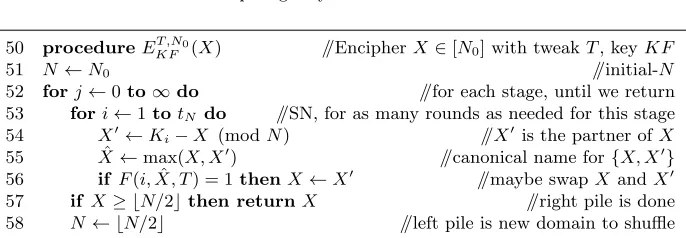
10 procedureEKFN (X) //invariant:X∈[N] 11 if N = 1then returnX //a single card is already shuffled
20 fori←1totN do //SN, fortN-rounds 21 X←Ki−X (modN) //Xis the “partner” ofX 22 Xˆ ←max(X, X) //canonical name for{X, X}
23 if F(i,Xˆ) = 1thenX ←X //maybe swapX andX
30 if X < pN then returnEpN
KF
X //recursively shuffle the first pile 31 if X≥pN then returnX //but second pile is done
Fig. 1. ConstructionSR =SR[SN]. The method enciphers on [N0] (the initial value ofN), each stage (recursive invocation) employingtN-rounds of SN (lines 20–23). The split values, pN, are a second parameter on which SR depends. The randomness for SN is determined byF:N×N→ {0,1}andK:N→N.
εN0 of uniform. Regardless of the values of these cards the second stage brings
the conditional distribution of the preceding qN1 cards to within distance εN1
of uniform, and so on. Therefore, applying Corollary 2 (as explained in the argument immediately following the statement of Corollary 2) shows that the final permutation is within δ of a uniform random permutation, where δ =
εN0+εN1+· · ·+εNn.
Using SN as the inner shuffle. We’ll write SR (no bold) for SR[SN], the sometimes-recurse transformation applied to the swap-or-not shuffle. The algorithm is shown in Fig. 1, now written out in the manner of a cipher, where the trajectory of a single card X is followed. Of course SN = SNt depends on the round count and SR =SRp depends on the split, so SR = SRt,p depends on both. The canonical choice for the splitpN ispN =N/2; when no mention ofpN is made, this is assumed. There is no default for the round countstN; we must select these values with care.
We proceed to analyze SR, for the canonical split, with the help of Proposi-tion 3 and equaProposi-tion (2). We aim to shuffleN cards to within a target distanceε. Assume we run each stage (that is, each SN shuffle) withtN adequate to achieve errorε/n for any half, rounded up, of the cards. WhenN is a power of 2, the expected total number of rounds to encipher a point will then be
E[TSR(N, ε)]≤TSN(N,N2,lgεN) +T SN(N
2,N4,lgεN)
2 +
TSN(N
4,N8,lgεN) 4 +· · · ≤2(7.23 lgN+ 4.82 lg lgN−4.82 logε) from (2)
ΔubSN(N, N/2, r) is increasing inN. Thus, for anyN,
E[TSR(N, ε)]≤14.46 lgN+ 4.82 lg lg 2N−4.82 lgε+ 14.46 (3) ∈Θ(lgN−lgε)
The worst-case number of rounds is similarly bounded. We summarize the result as follows.
Theorem 4. For any N ≥ 1 and ε ∈ (0,1), the SR construction enciphers points on[N]in Θ(lgN−lgε) expected rounds andΘ(lg2−lgNlgε)rounds in the worst case. No adversary can distinguish the construction from a uniform permutation on[N]with advantage exceedingε. This assumes uniformly random round keys and round functions for SN, appropriate round counts tN, and the canonical split.
As a numerical example, equation (3) gives E[TSR(1016,10−10)]≤1159. In the next section we will do better than this—but not by much—by doing calculations directly from equation (1) and by partitioning the error εso as to give a larger portion to earlier (that is, larger) generatedN.
5
Parameter Optimization
Round counts. Let us continue to assume the canonical split ofpN =N/2 and look at the optimization of round countstN under this assumption.
In speaking below of the numberpof nontrivial stages of SR, we only count generatedN-values withN ≥3. This is because we will always selectt2= 1, as this choice already contributes zero error, and the degenerate SR stage withN = 1 contributes no error and needs no t1 value (lett1= 0). Corresponding to this convention for counting the number of nontrivial stages, we letG(N0) =G(N0)\ {1,2} be the generatedN-values when starting with N0 but excluding N = 1 andN = 2.
Given an initialN0 and a targetε, we consider two strategies for computing the round countstN forN ∈ G(N0). Both use the upper boundΔubSN(N, q, r) = (2N3/2/(r+ 2))·((q+N)/(2N))r/2+1 onΔSN(N, q, r) given by equation (1).
1. Split the error equally. Let n = |G(N0)| ≈ lgN0 be the number of non-trivial stages. For each N ∈ G(N0) let tN be smallest number r for which ΔubSN(N,N/2, r)≤ε/n. This will result in rounds countstN that diminish with diminishingN, each stage contributing about the same portion to the error.
2. Constant round count. Letr0 be the smallest number r for which the sum N∈G(N0)Δ
ub
SN(N,N/2, r)< ε, and lettN =r0 for allN ∈ G(N0). This will result in stages that contribute a diminishing amount to the error.
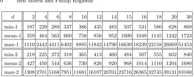
d 2 4 6 8 10 12 14 15 16 18 20 30
min-1 187 239 289 337 386 435 483 507 531 580 628 869
mean-1 359 464 563 660 758 856 952 1000 1048 1145 1242 1723
max-1 1110 2442 4411 6402 8885 11842 14790 16639 18239 22158 26069 51453
min-2 218 225 272 318 365 413 460 484 507 555 602 840
mean-2 427 450 544 636 730 826 920 968 1014 1110 1204 1680
max-2 1308 2701 5168 7951 11681 16107 20701 23716 26365 32745 39131 83160
Fig. 2. Speed of SR shuffle. Minimum, mean (rounded to nearest integer), and maximum number of rounds to SR-encipher a d-digit decimal string with error ε ≤
10−10and round countstN selected by strategy 1 or strategy 2, as marked. The split ispN=N/2. Round-counts for MC always coincide with the max-labeled rows.
and max round counts (a factor exceeding 17 when n= 16) coincides with the saving of SR over MC. In contrast, there is only a modest difference in mean round-counts between the two round-count selection strategies.
In numerical experiments, more complex strategies for determining the round counts did not work better.
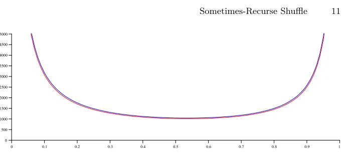
Non-equal splits. Besides the split of pN =N/2, we considered splits of pN =αNforα∈(0,1). For example, if the input is a decimal string then a selection of α= 0.1 corresponds to using SN until a 90% fraction of the cards are (almost) properly distributed, at which point there would be only a 10% chance of needing to recurse. When a recursive call is made, it would be on a string of length one digit less than before. But splits this uneven turn out to be inefficient; see Fig. 3. On the other hand, when the splitpN =αNhasα close to 1/2, the expected number of rounds is not very sensitive toα; again see the figure. Smallαmake each SN stage slower, but there will be fewer of them; largeαmake each SN stage faster, but there will be more.
Given the similar mean round counts for strategies 1 and 2, the similar mean round counts allαnear 1/2, the implementation simplicity of dividing by 2, and the better maximum rounds counts of strategy 1, the choice of strategy 1 and α= 1/2 seems best.
6
Incorporating Tweaks
Fig. 3. Selecting the split.Expected number of rounds (they-coordinate) to encipher
N = 1016 points using SR and a split ofpN =αN for variousα(thex-axis). The total variation distance is capped atε = 10−10. The top (blue) curve is with round countstN determined by for strategy 1; the bottom (red) curve for strategy 2. In both cases the smallest expected number of rounds occurs with a non-canonical split: 1048 rounds (α= 0.5) reduced to 1043 rounds (α= 0.53) for strategy 1; and 1014 rounds (α= 0.5) reduced to 1010 rounds (α= 0.52) for strategy 2.
credit card number, one might encipher only the middle six digits, using the first six and last four digits as the tweak.
The obvious way to incorporate a tweak in SR is to make the round constants Ki (line 21 of Fig. 1) depend on it, and to make the round functions F(i,Xˆ) (line 23 of Fig. 1) depend on it. Note, however, that an inefficiency emerges when the former is done: if there is a large space of possible tweaks, it will no longer be possible to precompute the round constantsKi. In addition, we do not want to get a security bound that gives up a factor corresponding to the number of tweaks used, which would be a potentially major loss in quantitative security.
As it turns out, neither price need be paid. In particular, it is fine to leave the round constants independent of the tweakT, and, even when doing so, there need be no quantitative security loss in the bound from making this change. What we call tweaked-SR, then, is identical to Fig. 1 except that the tweak T is added to the scope of F at line 23.
To establish security for this scheme, obtaining the same bounds as before, we go back to the swap-or-not shuffle and show that, in that context, if the round constants are left untweaked but the round function is tweaked, then equation (1) continues to hold. The result is as follows.
Theorem 5. Fix q1, . . . , ql with li=1qi =q. Let Xt1, Xt2, . . . , Xtl be SN
shuf-fles on G driven by the same round constants K1, . . . , Kr, but independent
round functions. Let Xt = (Xt1, . . . , Xtl). For i with 1 ≤ i ≤ l, let πi be
the uniform distribution on qi samples without replacement from G, and let
one each fromπ1, π2, . . . , πl. Let τ be the distribution ofXr. Then
τ−π ≤ 2N3/2 r+ 2
q+N
2N
r/2+1
. (4)
Proof. Let
Δ(j) = j−1 m=0 √ N 2 m+N
2N r/2
.
We show that
τ−π ≤Δ(q)
from which (4) follows by way of
τ−π ≤ q−1 m=0 √ N 2 m+N
2N r/2
≤N3/2 q/2N
0 (1/2 +x) r/2
dx
≤ 2N3/2 r+ 2
q+N
2N
r/2+1 .
For random variables W1, W2, . . . , Wj, we write τi( · |W1, W2, . . . , Wj) for the conditional distribution of Xi
r given W1, W2, . . . , Wj. Then Lemma 1 implies that
τ−π ≤ l
i=1
E τi(· |Xr1, . . . , Xri−1)−πi
. (5)
We claim that
E τi(· |Xr1, . . . , Xri−1)−πi
≤Δ(qi). (6)
For distributionsμandνthe total variation distance μ−ν is half theL1-norm of μ−ν. Since theL1-norm is convex, to verify the claim it is enough to show that
E τi(· |Xr1, . . . , Xri−1, K1, . . . , Kr)−πi
≤Δ(qi).
But the Xi
r are conditionally independent givenK1, K2, . . . , Kr, so τi(· |Xr1, . . . , Xri−1, K1, . . . , Kr) =τi(· |K1, . . . , Kr). Thus it remains to show that
E τi(· |K1, . . . , Kr)−πi ≤Δ(qi) = qi−1
m=0 √
N 2
m+N
2N r/2
but this inequality is shown on page 8 of [11]. This verifies (6), and combining this with (5) gives
τ−π ≤ l
i=1 Δ(qi)
≤Δ(q),
where the second inequality holds because the summands in the definition of Δ(j) are increasing. This completes the proof.
Theorem 5 plays the same role in establishing the security for tweaked-SR as equation (1) played for establishing the security of the basic version. The values in the table of Fig. 2, for example, apply equally well to the tweakable-SR.
We comment that in the the tweakable version of SR, the round constants do depend on the generatedN-values. This dependency can also be eliminated, but we do not pursue this for now.
7
Absence of Timing Attacks
With SR (and, more generally, withSR), the total number of roundst∗ used to encipher a plaintextX ∈[N0] to a ciphertext Y ∈[N0] will depend on X and the key K = KF. This suggests that an adversary’s acquiring t∗, perhaps by measuring the running time of the algorithm, could be damaging. But this is not the case—not in the typical setting, where the adversary knows the ciphertext— for, knowingY, one can determine the correspondingt∗ value.
It is easiest to describe this when N0 = 2n is a power of two, whence the generated N-values are 2n,2n−1, . . . ,4,2,1. Let t0, t1, . . . , tn−2, tn−1, tn be the corresponding round counts (the last two values are 1 and 0, respectively). Let t∗j =
i≤jti be the cumulative round counts: the total number of SN rounds if we run forj+ 1 stages. Thent∗is simplyt∗ whereis the number of leading 0-bits in then-bit binary representation ofY. The adversary holding a ciphertext ofY = 0z1Z, knows that it was produced usingt∗=t∗
zrounds of SN. Ciphertext 0n is the slowest to produce, needingt∗
n rounds.
The observation generalizes when N0 is not a power of 2: the set [N0] is partitioned into easily-calculated intervals and the number of SN rounds that a ciphertextY was subjected to is determined by the interval containing it.
8
Discussion
50 procedureET,N0
KF (X) //EncipherX∈[N0] with tweakT, keyKF
51 N←N0 //initial-N
52 forj←0to∞do //for each stage, until we return 53 fori←1totN do //SN, for as many rounds as needed for this stage 54 X←Ki−X (modN) //Xis the partner ofX
55 Xˆ ←max(X, X) //canonical name for{X, X}
56 if F(i,X, Tˆ ) = 1thenX ←X //maybe swapX andX
57 if X≥ N/2then returnX //right pile is done 58 N← N/2 //left pile is new domain to shuffle
Fig. 4. Alternative description of the tweaked construction. We eliminate the recursion and assume the canonical split. The valuestN again parameterize the algo-rithm, influencing the mechanism’s speed and the quality of enciphering.
Which pile to recurse on? The convention that SR recurses on the first (left) pile of cards, rather than on the second (right) pile of cards, simplifies bookkeeping: in this way, we will always be following a card X ∈ [N] for de-creasing values ofN. Had we recursed on the second pile we would be following a cardX ∈[N0−N+1.. N0−1] for decreasing values ofN. Concretely, the code in Figures 1 and 4 would become more complex with the recurse-right convention.
Multiple concurrent domains. Our assumption has been that the domain for the constructed cipher is [N0] for some N0. As with variable-input-length (VIL) PRFs, it makes sense to seek security against adversaries that can simul-taneously encipher points from any number of domains {[N0] : N0 ∈ N }, as previously formalized [3]. This can be handled by having the round-function and round-keys depend on the description of the domain N0. Once again it seems unnecessary to reflect the N0 dependency in the round-keys. To prove the con-jecture will take a generalization of Theorem 5.
Open question. The outstanding open question in this domain is whether there is an oblivious shuffle onN cards where a card can be tracked through the shuffle inworst-caseΘ(lgN)-time. Equivalently, can we do information-theoretic PRF to PRP conversion withΘ(lgN) calls, always, to a constant-output-length PRF?
Acknowledgments.This work was made possible by Tom Ristenpart and Scott Yilek generously sharing an early draft of their work [16]. Thanks also to Tom and Scott for their comments and interaction. Thanks to Terence Spies and Voltage Security, whose interest in FPE has motivated this line of work. Our work was supported under NSF grants CNS-0904380, CNS-1228828 and DMS-1007739.
References
2. Bellare, M., Impagliazzo, R.: A Tool for Obtaining Tighter Security Analyses of Pseudorandom Function Based Constructions, with Applications to PRP to PRF Conversion. ePrint report 1999/024 (1999)
3. Bellare, M., Ristenpart, T., Rogaway, P., Stegers, T., Format-Preserving Encryp-tion. In: Jacobson, J., Rijmen, V., Safavi-Naini, R. (eds.) Selected Areas in Cryp-tography (SAC) 2009. LNCS, vol. 5867, pp. 295–312. Springer, Heidelberg (2009)
4. Black, J, Rogaway, B.: Ciphers with Arbitrary Finite Domains. In: Preneel, B. (ed.) CT-RSA 2002. LNCS, vol. 2271, pp. 114–130. Springer, Heidelberg (2002)
5. Brightwell, M., Smith, H.: Using Datatype-preserving Encryption to Enhance Data Warehouse Security. 20th National Information Systems Security Conference Pro-ceedings (NISSC), pp. 141–149 (1997)
6. Did, user profile http://math.stackexchange.com/users/6179/did: Total Variation Inequality for the Product Measure. Mathematics Stack Exchange, http://math.stackexchange.com/q/72322(2011). Last visited 2014-02-06
7. Dworkin, M.: NIST Special Publication 800-38G: Draft. Recommendation for Block Cipher Modes of Operation: Methods for Format-Preserving Encryption. July 2013
8. FIPS 74: Guidelines for Implementing and Using the NBS Data Encryption Stan-dard. U.S. National Bureau of Standards, U.S. Dept. of Commerce (1981)
9. Granboulan, L., Pornin, T.: Perfect Block Ciphers with Small Blocks. In: Biryukov, A. (ed.) Fast Software Encryption (FSE 2007). LNCS vol. 4593, pp. 452–465. Springer, Heidelberg (2007)
10. H˚astad, J.: The Square Lattice Shuffle. Random Structures and Algorithms, 29(4), pp. 466–474. (2006)
11. Hoang, V., Morris, M., Rogaway, P.: An Enciphering Scheme Based on a Card Shuffle. In: Safavi-Naini, R., Canetti, R. (eds.) CRYPTO 2012. LNCS vol. 7417, pp. 1–13. Springer, Heidelberg (2012)
12. Liskov, M., Rivest, R., Wagner, D.: Tweakable Block Ciphers. J. of Cryptology, 24(3), pp. 588–613. Springer, Heidelberg (2011)
13. Morris, B.: The Mixing Time of the Thorp Shuffle. SIAM J. on Computing, 38(2), pp. 484–504 (2008)
14. Morris, B., Rogaway, P., Stegers, T.: How to Encipher Messages on a Small Domain: Deterministic Encryption and the Thorp Shuffle. In: Halevi, S. (ed.) CRYPTO 2009. LNCS vol. 5677, pp. 286–302. Springer, Heidelberg (2009)
15. Naor, M., Reingold, O.: On the Construction of Pseudo-Random Permutations: Luby-Rackoff Revisited. J. of Cryptology, 12(1), pp. 29-66 (1999)
16. Ristenpart, T., Yilek, S.: The Mix-and-Cut Shuffle: Small-Domain Encryptions Secure againstN Queries. In: Canetti, R., Garay, J. (eds.) CRYPTO 2013. LNCS vol. 8042, pp. 392–409. Springer, Heidelberg (2013)
17. Rudich, S.: Limits on the Provable Consequences of One-Way Functions. Ph.D. Thesis, UC Berkeley (1989)
18. Stefanov, E., Shi, E.: FastPRP: Fast Pseudo-Random Permutations for Small Do-mains. Cryptology ePrint Report 2012/254 (2012)
A
Proof of Lemma 1
We follow the approach outlined in [6] for bounding the total variation distance between two product measures. DefineV =V1×V2× · · · ×Vn. Note that
2 μ−ν = x∈V
|μ(x)−ν(x)| (7)
=
x∈V
|μ1(x)μ2(x)· · ·μn(x)−ν1(x)ν2(x)· · ·νn(x)|, (8)
where, forj with 1≤j ≤n, we define μj(x) to be μ(xj|x1, . . . , xj−1), with a
similar definition for νj(x). Forx∈V, definesj(x) as
μ1(x)μ2(x)· · ·μj(x)νj+1(x)· · ·νn(x). Then
s0(x) =ν1(x)ν2(x)· · ·νn(x) and sn(x) =μ1(x)μ2(x)· · ·μn(x),
and hence by the triangle inequality the quantity (8) is at most
x∈V n−1
j=0
sj+1(x)−sj(x) (9)
= n−1
l=0
x∈V
μl+1(x)−νl+1(x) μ1(x)μ2(x)· · ·μl(x)νl+2(x)· · ·νn(x). (10)
If we sum the terms over all x∈ V whose firstl components arex1, x2, . . . , xl we get
μ(x1, x2, . . . , xl)
v∈Vl+1
μ(v|x1, x2, . . . , xl)−νl(v|x1, x2, . . . , xl)
= 2μ(x1, x2, . . . , xl) μ(· |x1, . . . , xl)−ν(· |x1, . . . , xl) . Summing this overx1, . . . , xlgives
2E
μ(· |Z1, . . . , Zl)−ν(· |Z1, . . . , Zl)
![Fig. 1. Construction SR =ofsplit values, SR[SN]. The method enciphers on [N0] (the initial value N), each stage (recursive invocation) employing tN-rounds of SN (lines 20–23)](https://thumb-us.123doks.com/thumbv2/123dok_us/7901921.1311781/8.612.135.475.91.230/construction-ofsplit-values-enciphers-initial-recursive-invocation-employing.webp)