Transient Stability Analysis of Multi-machine
System during Different Fault Condition
Braj Kishor Shah, Shankar karki
IE(TU), BE (Scholar), Institute of Enginnering, Tribhuvan University, Nepal
BE(running), Western Region Campus, Institute of Engineering, Tribhuvan Universuty, Nepal
ABSTRACT: With the increasing electricity demand and growing complex power system, transient stability issues has been major threat to reliability measure of the power system. Systematic analysis of the system for findings of methods to further enhance system stability is the major need of the present. This paper aims to simulate in MATLAB and SIMULINK the behaviour of the system prior to the transient disturbance under which generator are subjected under oscillation in their rotor speed and integrate methods for the improvement. The paper presents classical model representation of the synchronous machine, two-axis synchronous machine along with excitation system and their dynamic characteristics. The system is subjected under different earth fault conditions and different fault duration upon which critical clearing time for the different instants is calculated through the time domain approach. The system generalized the importance of system variables and their significance in gaining back the synchronism and overview the idea of introducing improvement methods based upon those variables. Critical clearing computation enables relay setting for the given power system.
KEYWORDS: multimachine; transient stability; two axis modelling; earth fault; time domain approach; critical clearing time;
I.INTRODUCTION
The stability of power systems has been and continues to be of major concern in system operation. Modern electrical power systems have grown to a large complexity due to increasing interconnections, installation of large generating units.Monitoring the stability condition of a power system in real time has been recognized as a task of primary significance in preventing blackouts.Present trends in the planning and operation of power system have resulted in new kinds of stability problems along with financial and regulatory constraints. In this aspect, understanding the system behavior under steady and prior to disturbances allows power engineer to enhance the system .Broadly power system stability is defined as the property of a power system to remain in a state of operating equilibrium under normal operating condition and regain an acceptable state of equilibrium after being subjected to a disturbances[1].
Power system stability has been categorized into rotor angle stability and voltage stability. Rotor angle stability is the ability of the system to maintain synchronism and torque balance of synchronous machine. The stability is further analyzed under small signal stability and transient stability. Small signal stability deals system when subjected to small disturbances whereas transient stability is prior to the severe transient disturbances. Stability depends both on the initial operating conditions and severity of the disturbancesand is influenced by the non-linear power angle relationship [2]. A generator is an essential part in a power system, where its dynamics plays an important role in the dynamic performance of the system. It can be modeled with various levels of detail based on such factors as length of simulation, severity of disturbance, and accuracy required. Generally, synchronous machines are represented using detailed models, which include the influence of generator construction (damper windings, saturation, etc.), generator controls (excitation systems) [3].
This paper introduces a simple systematic approach for transient stability simulation.The proposed model uses MATLAB script for computing the initial parameters of SIMULINK blocks and for calculating the admittance matrices before, during and after fault occurrence based on the type and location of fault. The synchronous machine with its controller exciter system is modelled in Simulink and is considered as machine model.The power system can be easily extended, where the admittance of the passive network is considered and all machines are copied, and accordingly modified, from the described machine model.
The paper is organized as follows. In Section II, the Mathematical description of the system equations is introduced. In Section III, describe about the Simulink model. IV, model under study is presented with their data. Section V introduces results and discussion on the plot of rotor angle at different instant and their physical significance. Section VI concludes the idea of the paper.
II.MATHEMATICAL SYSTEM MODEL
This paper demonstrates the various electrical power system into mathematical form and analyse the system behaviour. Generator has been modelled as classical model and two axis model. The two model gives an overview of generator behaviour under steady and dynamic conditions. More variables have been taken into account under two axis modelling of the synchronous generator. Along this, excitation system has been modelled. IEEE type 1 exciter has been modelled. Under classical study, excitation has not been taken but under our proposed model excitation behaviour has been analysed and its response for the stability maintenance been studied. Network is reduced into simpler form for the easiness of the study and with the help of general power transfer function and differential equation of the swing simulation is carried out.
A. Generator modelling A.1 Classical Model
In this model each synchronous generator is being represented with a constant voltage source behind a direct axis transient reactance. Though under transient disturbance generator behaviour change dramatically this model doesn’t take into account the effect of saliency and assumes constant flux linkage. Three generators are represented as E1, E2 and E3 respectively [5].
A.2 . Two Axis model
Taking the effect of saliency into consideration the machine has been resolved into two axes namely, direct axis and quadrature axis. As the sub transient period only last for few cycles as compared to that of transient period, time constant for the sub transient period has been neglected. The overall system equations, including the differential-algebraic equations are expressed in the following general form [6]:
𝑉𝑞 = −𝑅𝑎𝐼𝑞+ 𝑋𝑑. 𝐼𝑑+ 𝐸𝑞 (1)
𝑉𝑑 = −𝑅𝑎𝐼𝑑− 𝑋𝑞. 𝐼𝑞+ 𝐸𝑑 (2)
𝐸𝑞′ = 𝑋𝑑− 𝑋𝑑′ 𝐼𝑑+ 𝐸𝑞 (3)
𝐸𝑑′ = − 𝑋𝑞− 𝑋𝑞′ . 𝐼𝑞+ 𝐸𝑑 (4)
𝑑𝐸𝑞 ′
𝑑𝑡 = −
1
𝑇_ 𝑑𝑜(𝑉𝑓+ 𝐸𝑞) (5)
𝑑𝐸𝑑′
𝑑𝑡 = −
1
𝑇𝑞𝑜′𝐸𝑑 (6)
𝐼𝑞 = 𝐼𝑐𝑜𝑠(𝛼 − 𝛿) (7)
𝐼𝑑 = 𝐼𝑠𝑖𝑛(𝛼 − 𝛿) (8)
𝑃𝑒𝑖 = 𝐸𝑑𝑖′ 𝐼𝑑𝑖+ 𝐸𝑞𝑖′ 𝐼𝑞𝑖 + 𝑋𝑞𝑖′ − 𝑋𝑑𝑖′ 𝐼𝑑𝑖𝐼𝑞𝑖 (9)
Equation (1) to (6) represents the dynamic equations performance of the synchronous machine. To the contrary, it a model comprising of the differential and the algebraic equations. In both model dynamics of turbine governor is being neglected and represented by a constant mechanical power Pm.
[I] = = 𝑛𝑘 =1[Y ][V ] (10) Where matrix [I] is the phasor currents injection into network nodes and matrix [V] is the phasor voltages at network nodes. n is the total no of generator at that system.
B. Excitation system modelling
As the machine is being represented by a constant voltage source behind the direct transient reactance the effect of dynamics of excitation system couldn’t be analysed. But addressing the dynamic behaviour of the machine, response of excitation system with its transient behaviour has been analysed. IEEE type -1 standard excitation system has been taken into study. The effect of stator winding saturation also has been taken into consideration.
Fig. II.2 shows a simplified schematic representation of used excitation system with voltage regulator. The entire excitation system is modelled with the combination of the transfer function [7].
𝑇𝐸𝑖′ 𝑑𝐸
𝑓𝑑𝑖
𝑑𝑡 = −(KEi+ 𝑆 𝐸𝑓𝑑𝑖 𝐸𝑓𝑑𝑖 + 𝑉𝑅𝑖 (11)
𝑇𝐴𝑖 𝑑𝑉𝑅𝑖
𝑑𝑡 = −VRi + 𝐾𝐴𝑖𝑅𝐹𝑖−
𝐾𝐴𝑖𝐾𝐹𝑖
𝑇𝐹𝑖 𝐸𝑓𝑑𝑖 + 𝐾𝐴𝑖(𝑉𝑟𝑒𝑓𝑖 − 𝑉𝑖) (12) 𝑇𝐹𝑖
𝑑𝑅𝐹𝑖
𝑑𝑡 = −𝑅𝐹𝑖+
𝐾𝐹𝑖
𝑇𝐹𝑖𝐸𝑓𝑑𝑖 (13)
Equation (11) represent the main excitation whereas equation (12) represent the secondary pilot excitation. Stabilization circuit is represented through transfer function as shown in equation (13).
C. Network Equation
In this simulation, load is represented as constant impedance type. By initial load flow calculation and determine each bus voltage magnitude and phase angle, current prior to disturbance is calculated as
In the classical model,
After load flow analysis by Newton Raphson method [8]
𝐼𝑖 = 𝑆𝑖∗ 𝑉𝑖 =
𝑃𝑖+𝑗 𝑄𝑖∗
𝑉𝑖 , i=1, 2, 3, …, m (14)
𝐸𝑖 = 𝑉𝑖+ 𝐽𝑋𝑑′. 𝐼𝑖 (15)
𝑦𝑖𝑜 = 𝑆𝑖∗ |𝑉𝑖|2=
𝑃𝑖−𝑗 𝑄𝑖
|𝑉𝑖|2 (16)
𝑃𝑒𝑖 = 𝑚𝑗 =1 𝐸𝑖′ 𝐸𝑗′ |𝑌𝑖𝑗|cos(θij− 𝛿𝑖+ 𝛿𝑗) (17)
𝐻𝑖 𝜋 𝑓𝑜
𝑑2𝛿𝑖
𝑑 𝑡2 = 𝑃𝑚𝑖 − 𝐸𝑖
′ 𝐸
𝑗′ |𝑌𝑖𝑗|cos(θij− 𝛿𝑖+ 𝛿𝑗) 𝑚
𝑗 =1 (18)
Equation (14) represent the flow of current at each bus. The mentioned classical model representation of the generator by the voltage behind the direct axis transient reactance is shown by the Equation (15). All loads are converted into equivalent admittance through the means of Equation (16). Equation (17) and (18) corresponds to the electrical power output of the respective machine and the solving of the swing equations respectively.
In the case of our proposed model we simulate our system with different three phase earth fault conditions. With the help of load analysis, each generator bus voltage is generated before, during and after fault conditions.[9]
𝑃𝑡𝑟𝑎 = 𝑉∗𝑉𝑡
𝑋 𝑠𝑖𝑛𝛿 (19) 𝑑𝛥𝜔
𝑑𝑡 =
𝜋𝑓 0
𝐻 (𝑃𝑚 − 𝑃𝑒) (20)
𝑑𝛿
The power transmission is the most influencing factor for the stability limit of the system. Prior to the before, during and after fault conditions the power transmission is given by the Equation (19). Equation (20) and (21) are the simplest form of equation (17) and (18) which is used for computation.
III.MODEL DISCRIPTION
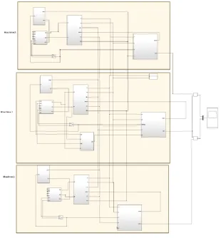
In this section, the whole system simulation is shown which is constructed by using the mathematical equations which described in above section. Simulation of each part of the machine is constricted by using their respective equations. The description is nine bus WSCC system. The detail of the system is given in [10].
Figure 0.1Overall system model
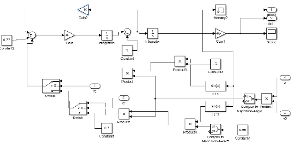
Figure 0.1Machine dynamic system model of each machine
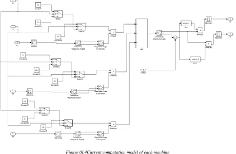
Figure 0I.4Current computation model of each machine
Figure 0I.5Excitation system model of each machine
flow. This arrangement of the model is simple and systematic, which is suitable for researchers or students to build the required network and to investigate the effect of the different fault location and different fault conditions i.e. different fault impedance.
IV. ILLUSTRATIVE SYSTEM EXAMPLE
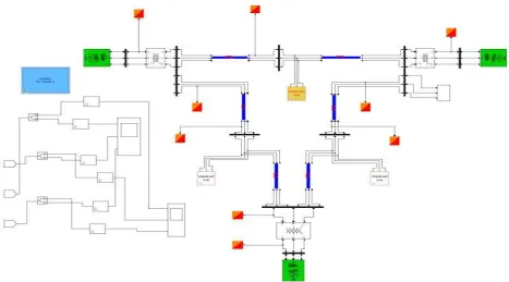
Figure IV.1 WSCC- 3 Machine 9 bus system
Western System Coordinated Council (WSCC) 3 machine, 9 bus system has been taken into study [11]. They are the system appearing in reference [12]. The base MVA is 100 and base frequency is 60.
V. RESULT AND DISCUSSION
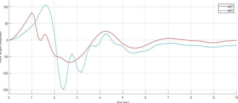
Figure V.2 proposed model tc=1.23s
Figure 0.3 proposed model tc=1.24s
Figure V.2 illustrates the relative rotor angle upon the clearance of the fault tc=1.24 sec. Here, machine 3 can’t get back
its synchronism resulting in the rapid increase of its rotor angle showing instability nature of it whereas still machine 3 able damp out the oscillation due to the different voltage level at the terminal of machine 2 as compare to terminal of machine 3.
Figure V.3 represents the relative rotor angle upon the clearance of the fault at tc=1.54 sec. It illustrates that both the
Figure V.4proposed model tc=1.54s
When thefault resistance is changed then the new voltage level during the fault is obtained through load flow analysis. The system is studied further with the new voltage level of 0.4p.u, 0. 42p.u and 0.25p.u of machine 1, machine 2 and machine 3 respectively. Figure V.4 and Figure V.5 illustrate the relative angular position under fault clearing time of 1.46 sec and 1.47 sec respectively. When tc = 1.46sec both the machine is stable and at tc = 1.47 sec the machine 2 became unstable rather than 3. The system is further simulated for next fault clearing and both the machine gets unstable at tc = 1.73sec as shown in Figure V.6. Thus, critical clearing time of the system is found to be 1.73 sec.
Figure V.5 Swing Curve at tc=1.47s
Figure V.6Swing Curve at tc=1.73s
Table 0.1 Critical clearing time instants
V1=0.31pu,
V2=0.35pu,
V3=0.2 pu
V1=0.4pu,
V2=0.42pu,
V3=0.25 pu
Tc=1.23sec
Stable: machine 2, machine 3
Unstable:
Tc=1.46sec Stable: machine 2,
machine 3 Unstable: Tc=1.24sec
Stable: machine 2 Unstable: machine 3
Tc=1.47sec Stable: machine 3 Unstable: machine 2 Tc=1.54sec
Stable: Unstable: machine 2,
machine 3
Tc=1.73sec Stable: Unstable: machine 2,
Figure V.7Swing Curve at tc=0.15s
Figure V.8Swing Curve at tc=0.16s
Figure V.7 and Figure V.8 shows the stability time limit of the same studied system under the classical model with the findings of critical clearing time of 0.16 sec. The simulation provides overview of the system behaviour under transient disturbance and effect of system variable in critical clearing time of the system.
VI.CONCLUSION
Methods and models for the study of transient stability have been presented in this paper. The results comparisons emphasize the need of accountability of detailed modelling and dynamic behaviour of excitation system for stability assessment. The proposed model is better suited for the stability analysis along with inclusion of damping and the excitation(saturation) in the stability of the system. The voltage level during the occurrence of the fault influenced by the fault impedance is affected the critical clearing time of the system. Although the proposed model is introduced to study transient stability at the different machine nature as well as different fault condition, different analysis is tested and will be introduced as a future work. Furthermore, by using this this model also can analyse the effect of excitation system and it’s time constant on the critical time of the transient stability.
REFERENCES
[1] Kundur P. Power system stability and control. In: EPRI power system engineering series. New York: Mc Graw-Hill, 1994. [2] L. Grigsby, Electric Power Engineering Handbook, 2nd ed. CRC Press, May 2001.
[3] T. Hiyama, Y. Fujimoto, and J. Hayashi, “MATLAB / Simulink based transient stability simulation of electric power systems,” in Power Engineering Society 1999 Winter Meeting, IEEE, vol. 1. IEEE, 1999, pp. 249–253.
[5] Saadat, Hadi, Power System Analysis, New Delhi, Tata McGraw-Hill Publishing Company Limited, 2002. [6] L.P. Singh, Advanced Power System and Dynamics. New Age International, 2006.
[7] Sauer PW and Pai MA. Power system dynamics and stability. New Jersey: Prentice Hall, Upper Saddle River, 1998.
[8] Patel R, Bhatti TS and Kothari DP., "MATLAB / SIMULINK based transient stability analysis of a multimachine power system," Interntional Journal of Electrical Engineering Education, vol. 39, pp. 320-336, 2002.
[9] J. Duncan Glover, Mulukutla S. Sarma and Thomas J. Overbye. Power System Analysis and Design. Cengage Learning, sixth edition, 2015. [10] DivyaAsija, Pallavi Choudekar, K.M.Soni, S.K. Sinha, "Power Flow Study and Contingency status of WSCC 9 Bus Test System using
MATLAB" International Conference on Recent Developments in Control, Automation and Power Engineering (RDCAPE), PP. 339, 2015 [11] Harrys Kon. 2016. WSCC 9-Bus System. [ONLINE] Available at: https://harryskon.com/2016/02/28/wscc-9-bus-system/
[12] Anderson PM and Fouad AA. Power system control and stability. Stevenage: IEEE Press, 2003.
[13] Ekinci, S., Zeynelgil, H.L., Demiroren, A., "A didactic procedure for transient stability simulation of a multimachine power system utilizing SIMULINK," Interntional Journal of Electrical Engineering Education, pp.53(1), 2016.
Appendix I
Notations Meaning
D Damping coefficient E’d d-axis transient voltage
Efd excitation system voltage
E’q q-axis transient voltage
𝛿 Rotor angle position θ Angle of terminal voltage ω Rotor angle speed ωs Synchronous angular speed
TF stabilizer circuit time constant
TA regulator time constant
Iq q-axis armature current
KA regulator gain
KE exciter gain
KF stabilizer circuit gain
Pe electrical output power
Pm mechanical input power
Rs armature resistance
S(Efd) exciter saturation function
T’do d-axis open circuit time constant
TE exciter time constant
yaf admittance matrix after fault clearing
ydf admittance matrix during fault ybf fault admittance matrix before fault ωs Synchronous angular speed
H inertia constant of generator Id d-axis armature current
V generator terminal voltage ω Rotor angle speed
T’qo q-axis open circuit time constant
Appendix II
Yaf=[ 1.1064-4.6974i0.1643+2.2743i-0.0648+ 2.2479i 0.1643+2.2743i1.1418-2.8688i-0.0177+0.4030i -0.0648+2.2479i -0.0177+0.4030i0.5591-2.4474i]; Ydf=[1.1290-5.1240i0.1041+1.7237i 0+0.000001i 0.1041+1.7237i 0.7175-5.772i 0+0.000001i 0+0.000001i0+0.00001i -17.0648i];