An Exclusive Faulty Node Detection in Mobile Wireless Network

(1)

An Exclusive Faulty Node Detection in Mobile Wireless Network

A.Mounika

1

_{, Shaik Reshma}

2

1 M.Tech Student, Department of CSE, Dr.K.V.Subba Reddy College of Engineering for Women, Kurnool, Ap. 2 Assistant Professor, Department of CSE, Dr.K.V.Subba Reddy College of Engineering for Women, Kurnool, Ap.

Abstract: In this paper, we propose a novel probabilistic approach that judiciously combines localized monitoring, location estimation and node collaboration to detect node failures in mobile wireless networks. Specifically, we propose two schemes. In the first scheme, when a node A cannot hear from a neighboring node B, it uses its own information about B and binary feedback from its neighbors to decide whether B has failed or not. In the second scheme, A gathers information from its neighbors, and uses the information jointly to make the decision. The first scheme incurs lower communication overhead than the second scheme. On the other hand, the second scheme fully utilizes information from the neighbors and can achieve better performance in failure detection and false positive rates and incur low communication overhead.

Key words: Mobile Wireless Networks, Node Failure, Node Failure Detection, Network Management, Fault Management.

I. INTRODUCTION

Mobile wireless networks have been used for many mission critical applications, including search and rescue, environment monitoring, d isaster relief, and military operations. Such mobile networks are typically formed in an ad-hoc manner, with either persistent or intermittent network connectivity. Nodes in such networks are vulnerable to failures due to battery drainage, hardware defects or a harsh environment. Node failure detection in mob ile wireless networks is very challenging because the network topology can be highly dynamic due to node movements. Therefore, techniques that are designed for static networks are not applicable. Secondly, the network may not always be connected. Therefore, approaches that rely on network connectivity have limited applicability. Th ird ly, the limited resources (computation, communication and battery life) demand that node failure detection must be performed in a resource conserving manner. Node failure detection in mobile wireless networks assumes network connectivity. Many schemes adopt probe-and-ACK (i.e., ping) or heartbeat based techniques that are common ly used in distributed computing. Probe-and-ACK based techniques require a central monitor to send probe messages to other nodes. When a node does not reply within a timeout interval, the central monitor regards the node as failed. Heartbeat based techniques differ fro m p robe-and-ACK based techniques in that they eliminate the probing phase to reduce the amount of messages. Several existing studies adopt gossip based protocols, where a node, upon receiving a gossip message on node failure information, merges its information with the information received, and then

broadcasts the combined in formation. A co mmon drawback of probe-and-ACK, heartbeat and gossip based techniques is that they are only applicable to networks that are connected. In addition, they lead to a large amount of network-wide monitoring traffic. In contrast, our approach only generates localized mon itoring traffic and is applicable to both connected and disconnected networks.

II. EXISTING A ND PROPOSED SYSTEMS A.Exis ting System

One approach adopted by many existing studies is based on centralized mon itoring. It requires that each node send periodic “heartbeat” messages to a central monitor, which uses the lack of heartbeat messages from a node (after a certain timeout) as an indicator of node failure. Th is approach assumes that there always exists a path from a node to the central monitor, and hence is only applicable to networks with persistent connectivity. Another approach is based on localized monitoring, where nodes broadcast heartbeat messages to their one-hop neighbors and nodes in a neighborhood monitor each other through heartbeat messages. Localized monitoring only generates localized traffic and has been used successfully for node failure detection in static networks.

B. Pro posed System

In this paper, we propose a novel probabilistic approach that judiciously comb ines localized monitoring, location estimation and node collaboration to detect node failures in mobile wireless networks. Specifically, we p ropose two schemes. In the first scheme, when a node A cannot hear fro m a neighboring node B, it uses its own information about B and binary feedback fro m its neighbors to decide whether B has failed or not. In the second scheme, A gathers information fro m its neighbors, and uses the information jointly to make the decision. The first scheme incurs lower communication overhead than the second scheme. On the other hand, the second scheme fu lly utilizes information fro m the neighbors and can achieve better performance in failure detection and false positive rates.

1. A d vantages of Proposed System

Simu lation results demonstrate that both schemes achieve high failure detection rates, low false positive rates, and incur low communication overhead.

Our approach has the advantage that it is applicable to both connected and disconnected networks.

International Journal of Research

Available at https://edupediapublications.org/journals

e-ISSN: 2348-6848 p-ISSN: 2348-795X Volume 04 Issue 13

(2)

Co mpared to other approaches that use localized monitoring, our approach has similar failure detection rates, lower co mmun ication overhead and much lower false positive rate.

Our approach only generates localized monitoring traffic and is applicable to both connected and disconnected networks.

Fig .1. System A rchitecture

C. M o dules

We have 3 main Modules.

Localized Monitoring Module Location Estimation Module Node Collaboration Module

1. M o dule Description

Localized Monitoring: Localized mon itoring only generates localized traffic and has been used successfully for node failu re detection in static networks.

Location Estimation: By localized monitoring, Node only knows that it can no longer hear fro m other neighbor nodes, but does not know whether the lack of messages is due to node failure or node moving out of the transmission range. Location estimation is helpfu l to resolve this ambiguity.

Node Co llaboration: Through this module, we can improve the decisions which are taken during Location estimation module.

III. PERFORMANCE EVALUATION

We evaluate the performance of our schemes through extensive simu lations using a purpose-built simulator. The simu lator is built using Matlab. The main reason for using the purpose built simu lator instead of other simu lators (e.g., ns3 [2]) is because it provides much more flexib ility in implementing the node failu re detection algorith ms that are proposed in the paper. Imp lementing location estimation (an important part of our algorithms) presented-B3 is particularly convenient in Matlab (because of many readily available mathematical libraries) than that in other network simu lators. In the following, we first describe the simulation setting, and then describe the evaluation results.

A . Simu lation Setting

In all the simulations, the nodes move in a 500m × 500m square area. The total nu mber of nodes, N, is varied fro m 20 to 150. The in itial locations of the nodes follow a 2D Poisson distribution. The transmission range of a node is circular with the radius, r, varied fro m 30m to 130m (our schemes can be applied to irregular transmission ranges; evaluation under those settings is left as future work). The above combination of parameters leads to a wide range of neighborhood density for evaluating our approach (see the range of neighborhood density). We evaluate our schemes with three mobility models: the rando m waypoint model [9], the smooth random model [7] and the Levy walk model. The random waypoint model is widely used in mobile network studies. We have applied the fix described to overcome its limitations. The smooth random model is a variant of the random waypoint model in that it changes the speed and direction of node movement incrementally and smoothly. The Levy walk model is reported to contain some statistical similarity to human walks, where the travel distance (i.e., flight length) of each movement follo ws a heavy-tail distribution. Each node sends a burst of K heartbeat messages in each time unit of δ seconds. We also refer to the time un it as the heartbeat interval, and use the terms interchangeably. For simp licity, we assume independent node failures and packet losses. In addition, we assume homogeneous node failure probability and packet loss probability. We remark that our schemes do not have these assumptions.

(3)

Because of the homogeneity assumption, we omit failed, A simply suspects that B has failed and sends an superscripts and use pd and pc to represent node failure inquiry to its neighbors. If none of A’s neighbors reply that

probability and packet loss probability, respectively. In our B is alive, then A sends a message to the manager node that simulations, pd is varied from 0.01 to 0.05; pc is varied from B has failed. In the following, we first report the results

0.001 to 0.1. The above choices of pd and pc cover a wide when the heartbeat interval is one second (i.e., δ = 1 sec), range of settings. Our scheme also works for higher or lower assuming the failure and packet loss probabilities are known

pd; we briefly describe the cases of larger pc (larger pc can and the standard deviation of the location measurement error lead to lower confidence in detecting failures). We assume is 1m. We then investigate the impact of probability

that pd and pc are not known, but can be estimated. The estim ation erro rs, locatio n meas ur em ent error s, and heartb eat maximu m relative estimation error is denoted as err. The interval. We only report the results under random waypoint location measurement error is assumed to be zero mean model; the results under the smooth random model are

Gaussian white noise with the standard deviation, σw (refer similar.

to), varied from 1m to 10m. There is no interference model Choice of Threshold θ: We set the detection threshold, in the simulator. Adding an interference model will lead to θ, to 0.7, 0.8 or 0.9, and observe similar results (as different characteristics of packet losses, which is left as explained). All the results presented below use θ = 0.8. future work. In each simulation run, we start with a warm-up Choice of K: To deal with packet losses, a node sends a

phase of 20 seconds and then simulate node failures. For burst of K heartbeat messages in each time unit. For the simplicity, node failures are simulated at each time unit, and binary feedback scheme, we can derive the minimum K

we stop the simulation when at least one node fails. For each that is needed for failure node detection from the setting, we repeat the simulation at least 100 times, and necessary condition. Specifically, under our assumption

present the average results; the confidence intervals are tight of indepen dent pack et losses, pc, K = pKc, and we have and hence omitted for clarity. The performance metrics are

≥

l og ⁡( / − )− 1−

(1) (1) detection rate, defined as the number of failures that are

detected successfully divided by the actual number of For instance, when θ = 0.8 and pd = 0.01, the minimum failur es , (2) false positiv e rate, defin ed as the number of false K is 1, 2 and 3 for pc = 0.001, pc = 0.05 and pc = 0.1, alarm s (i.e., a node is considered to be failed but actually it is respectively. For all the settings we explored, a small value

not) divided by the number of alarms that are raised, and (3) of K (no more than 3) is sufficient to achieve good communication overhead, defined as the average number of perfo rm an ce. The abov e is for indep end ent losses. When that messages sent per second during the entire detection period. is not the case (i.e., pc, K > pKc), the minimum K can be We evaluate the performance of both of our schemes. In the larger than that under independent losses. For the non-binary

following, we mainly report the performance of the binary feed back schem e, we can deriv e the minim u m K that is feedback scheme, and “our scheme” henceforth refers to this needed for failure node detection from the necessary

scheme. The non-binary scheme mainly differs from the condition. Specifically, under our assumption that p(i)c,K = binary schem e in the minimum required K for effective pc, K = pKc,∀i, we hav e

/ − −log ⁡(1− )

failure node detection and communication overhead, ≥

l og

(2) simulation results on these two aspects are, respectively. In _{Comparing (1) and (2), it is easy to see that the minimum} the following, we present evaluation results under the _K_{required for the non-binary scheme can be significantly}

random waypoint model and the smooth random model, first _{smaller than that for the binary scheme. For instance, our} in connected networks and then in disconnected networks.

simulation results show that when pd = 0.01; pc = 0.01; N = At the end, we briefly present the results under the Levy

8 0 , an d r = 8 0m, the b in ary scheme req uires K ≥ 2, while

walk model.

th e n o n -binary sch eme on ly req uires K ≥ 1. Last, fo r a giv en

B. Ev aluation Results for Connected Networks scenario, both the binary and non-binary schemes can achieve high failure detection rate and low false positive rate The evaluation setting for connected networks is

using the minimum required K derived from (1) and (2) motiv ated by the robotic sensor network application. The _{respectively.}

netw or k is connected at every point of time. A manag er node is in the central region of the area. Node failure alarms are sent to the manag er node. We consid er three node movem ent speed ranges: low speed range of [1; 5]m/s, medium speed range of [5; 10]m/s , and high speed range of [10; 15]m /s. We compare our scheme to two schemes, referred to as centralized and localized schem es, motiv ated by the schem es in [6], and the scheme, respectively. In the centralized scheme, each node sends periodic heartbeat messages to the manager node, which decid es that a node has failed when not hearing from the node. The localized scheme differs from our scheme only in that it does not calculate the probability

of node failure. Specifically, when node A no longer hears _{F ig .2 . D etectio n R ate an d False Positive Rate o f Our} from node B, instead of calcu latin g the probability that B has

Sch eme (K = 2, pc = 0.01, pd = 0.01, σw = 1m, low speed).

International Journal of Research

(4)

C. Detection Rate and False Positive Rate

In our setting, the neighborhood density ρ = πr2N/S, where S = 500m×500m. Figs 2(a) and (b) p lot the detection rate and false positive rate of our scheme versus neighborhood density when K = 2, pc = 0.01, pd = 0.01, and nodes move at lo w speed. The various neighborhood densities are obtained using the combinations of r (ranging fro m 30m to 140m) and N (ranging fro m 20 to 140). For clarity, we only plot the results for the combinations leading to neighborhood density of at least 1. In Fig. 2(a), we also plot the upper bound of the failure detection rate, since for the random waypoint model the node distribution can be well appro ximated by a 2D Po isson distribution [8]. Observe that the detection rates of our scheme are very close to the upper bound, indicating that our scheme achieves very good detection rates. As expected, the detection rate increases while the false positive rate decreases with neighborhood density. Specifically, when the neighbor density is above 3, our scheme achieves a detection rate of above 0.9 and a false positive rate of below 0.02. The performance is worse when nodes move faster (figures omitted). This is expected. Consider an arbitrary node, A, that is in the neighborhood of node B at time t. When nodes move fast, A is mo re likely to be out of the range of B at time t+1, which is more likely to lead to missed detections (when B fails) or false positives (when B does not fail). We next co mpare the detection rate and false positive rate of our scheme and the other two schemes. Under ideal network conditions (i.e., packet delays and losses are negligible), the centralized scheme can always detect failed nodes and does not cause false alarms. On the other hand, as we shall see, its communication overhead is much h igher than that of our scheme. The detection rate of the localized scheme is no less than that of our scheme since when our scheme detects a node failure, the localized scheme can detect that node failure as well. Ho wever, the localized scheme suffers fro m many mo re false positives. Fig. 3 p lots the detection rate and false positive rate of our scheme and the localized scheme when the transmission range is varied fro m 60 to 130m, and the nu mber of nodes in the area is 80. We observe that the detection rate of our scheme is slightly lower than that of the localized scheme, while the false positive rate of our scheme is much lower than that of the localized scheme. Fo r instance, when r = 60m, the false positive rate under our scheme is 0.01 versus 0.27 under

Fig.3. Co mparing Detection Rate and False Positive Rate of Ou r Scheme and the Localized Scheme (K = 2, N = 80, pc = 0.01, pd = 0.01, σw = 1m, high speed).

Fig.4. An Examp le That Illustrates False Positives in the Lo calized Scheme

the localized scheme. We also plot the results for the non binary feedback scheme, wh ich has slightly better performance than the binary feedback scheme. The much lower false positive rate under our scheme is because of its ability to differentiate a node failure fro m the node moving out of the transmission range, while the localized scheme cannot differentiate these two cases. Fig. 4 shows an example observed in the simu lations. Nodes A and B are within each other’s transmission range at time t, and are out of each other’s transmission range at time t+1. In the localized scheme, since A cannot hear from B at time t+1, it suspects that B has failed, and broadcasts an inquiry to its one-hop neighbors. Since none of A’s neighbors is in B’s transmission range at time t + 1, A does not hear anything fro m its neighbors about B, and concludes that B has failed. Similarly, B concludes that A has failed. Therefore, the localized scheme leads to two false positives in this examp le. Our scheme does not lead to any false positive since A finds the probability that B has failed is below the threshold, and hence does not suspect that B has failed; similarly, B does not suspect that A has failed.

D. Co mmu nication Overhead

Let H denote the average number of hops from a node to the manager node. The centralized scheme leads to an average of N×K×H messages in each time unit, where N is the number of nodes and K is the number of heartbeat messages per time unit. In our scheme and localized s cheme, the number of heartbeat messages is N × K in each time unit, significantly lower than that of the centralized scheme especially when H is large. In addition to heartbeat messages, our scheme and the localized scheme also lead to two other types of messages: one is the localized inquiries and responses during node collaboration (on average

(5)

Fig.5. Co mmunication Overhead o f the Th ree Schemes (K = 2, Pc = 0.01, Pd = 0.01, Σw = 1m, N = 120, High Speed).

Fig.6. Impact of Estimation Errors in pd (K = 2, pc = 0.01, pd

= 0.03, r = 80m, σw = 1m, High Speed).

We observe that the centralized scheme leads to much higher commun ication overhead than our scheme. Furthermore, the localized scheme also leads to higher communication overhead than our scheme, wh ich is due to two reasons. First, the localized scheme has more inquiries and responses during node collaboration. Suppose node A hears fro m node B at time t but not at time t+1. In the localized scheme, A will suspect that B has failed, lead ing to an inquiry fro m A and the corresponding responses from A’s neighbors. In our scheme, A only sends an inquiry when the failure probability of B is larger than the threshold. Secondly, the localized scheme leads to more alerts to the manager node due to more false alarms. Of all the settings we exp lore, when the neighborhood density is larger than 3, the communication overhead of the centralized scheme is 3.4 to 5.0 times as large as that of our scheme; the communication overhead of the localized scheme is 1.9 to 2.3 times as large as that of our scheme. In the above, “our scheme” refers to the binary feedback scheme. Fig. 5 also plots the results for the non-binary feedback scheme when K

= 2 and K = 1, respectively.

Fig.7. Impact of Estimation Errors in pc (K = 2, pc = 0.03, pd

= 0.01, r = 80m, σw = 1m, High Speed).

As explained in Section III-B2, the non-binary scheme requires K≥ 1 wh ile the b inary scheme requires K≥ 2 for this setting. When K = 2, the commun ication overhead of the non binary scheme using is larger than that of the binary scheme, while is lower than that of the localized scheme. When K = 1, the non-binary scheme leads to lo wer overall communication overhead compared to the binary scheme that uses K = 2 because the number of heartbeat messages is reduced by half. Last, note that with the nu mber of nodes fixed the centralized scheme’s commun ication overhead decreases with the transmission range (due to shorter routes to the manager node), wh ile for our scheme and localized scheme, the co mmunication overhead increases with the transmission range due to more nodes in the neighborhood and hence more responses during node collaboration. Th is indicates the tradeoffs between schemes that use centralized monitoring and those using localized monitoring. If the transmission range is large enough that the routes to the manager node are comparatively short (meaning that the effective neighborhood density is high), it might be beneficial to use schemes based on centralized mon itoring, and vice versa.

E. Imp act of Probability Estimation Errors

We now investigate the impact of estimation errors in pd

and pc on the performance of our scheme. The relative estimation error is up to 66.6%. We next present results under two settings where the relative estimation error is 66.6%. In Fig. 6, the actual pd is 0.03, while the estimated pd

is 0.01 or 0.05. We observe that the performance of our scheme when using the estimated pd is similar to that when using the actual pd. Fig.7 plots the performance of our scheme when the actual pc is 0.03, wh ile the estimated pc is 0.01 or 0.05. We again observe similar performance when using the estimated pc and the actual pc. Th is demonstrates that, as explained, our scheme is not sensitive to estimation errors in pc and pd. We have also investigated the cases when both the estimates of pd and pc have erro rs. The results again confirm that our scheme is not sensitive to estimation errors in pd and pc (figures omitted).

International Journal of Research

(6)

heartbeat intervals also lead to longer delays in detecting node failures, which is undesirable for many applications.

Fig .8. Impact of Location Measurement Deviation (K = 2, pc

= 0.01, pd = 0.01, r = 80m, N = 100).

1. Impact of Location Measurement Errors: Fig. 8(a) plots the detection rate of our scheme while increasing σw, the

standard deviation of the measurement noise, fro m 1m to 10m. The results under both low and high movement speeds are shown in the figure. We observe that when increasing σw, the detection rate first decreases slowly, and then

decreases sharply when σw is above a certain value. This

indicates that our scheme can tolerate inaccuracy in location measurements. Fig. 8(b) plots the false positive rate of our scheme versus σw. When increasing σw, the false positive

rate under lo w speed remains low wh ile the false positive rate under high speed decreases. This is consistent with the lower detection rates when increasing σw: when location prediction is inaccurate, the confidence in node failure probability is lo w, leading to missed detections as well as fewer false positives.

2. Impact of Heartbeat Interval: So far all the results are obtained when the heartbeat interval is one second. When increasing the heartbeat interval, the co mmunication overhead decreases. On the other hand, the location estimation beco mes less accurate. In addition, a node, A, in the neighborhood of another node, B, is more likely to be outside of the neighborhood of B in the next heartbeat interval. Both factors may have adverse impact on the detection rate and false positive rate. Fig.9 plots the detection rate and the false positive rate of our scheme when increasing the heartbeat interval fro m 1 to 10 seconds. As expected, the detection rate and the false positive rate degrade more slowly when node speeds are low, while degrade more quickly when node speeds are high. Fig. 10 plots the communication overhead when increasing the heartbeat interval. As expected, the co mmunication overhead decreases when increasing the heartbeat interval. On the other hand, when the heartbeat interval is large, inaccurate location estimation leads to more inquiries and responses as well as more messages to the manager node (due to increased false positive rate), causing the gain in communication overhead to level off. The above indicates that it is not beneficial to set the heartbeat interval too large, especially when nodes move fast. In fact, in addition to degraded detection rate and false positive rate, larger

Fig.9. Impact of Heartbeat Interval on Detection Rate and False Positive Rate of Our Scheme (K = 2, pc = 0.01, pd = 0.01, r = 80m, N = 100, σw = 1m).

Fig.10. Impact of Heartbeat Interval on Co mmunication Overhead of Our Scheme (K = 2, pc = 0.01, pd = 0.01, r = 80m, N = 100, σw = 1m).

F. Ev aluation Results in Disconnected Networks

The evaluation setting for disconnected networks is motivated by the hiking application. We consider low movement speed of [0.4-0.6]m/s and transmission range of 50m. The nu mber of nodes is varied fro m 30 to 100. There are 10 sinks distributed uniformly randomly in the 500m×500m area. The sinks are connected to a manager node located in the central region of the area. Due to low node density, the network only has intermittent connectivity. We use the following routing strategy. Suppose that node A generates an alarm that B has failed at time t. Then A transmits this message to all of its current neighbors. Each of these nodes (A and its neighbors) carries the information; when one of them meets a sink, it uploads the information to the sink, which in turn relays the information to the manager node. In addition to performance metrics described earlier, we consider another metric, discovery delay, which is the delay fro m when a node is found to be failed to when the message reaches the manager node (we assume neglig ible delay fro m a sink to the manager node). We only report the results under random waypoint model; the results under the smooth random model are similar.

(7)

communication overhead (up to 80% lower). In addition, our approach has the advantage that it is applicable to both connected and disconnected networks. Co mpared to other approaches that use localized mon itoring, our approach has similar failure detection rates, lower co mmunication overhead (up to 57% lower) and much lower false positive rate (e.g., 0.01 versus 0.27 in some setting).

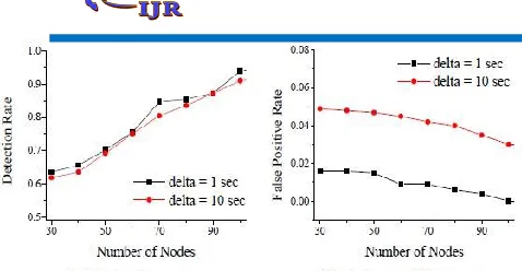
Fig.11. Detection Rate and False Positive Rate in Disconnected Networks (K = 2, pc = 0.01, pd = 0.01, r = 50m, σw = 1m).

Fig.12. Co mmunication Overhead and Discovery Delay In Disconnected Networks (K = 2, pc = 0.01, pd = 0.01, r = 50m, σw = 1m).

Fig. 11 plots detection rate and false positive rate under two heartbeat intervals, δ = 1 and 10 seconds. The false positive rate under δ = 1 second is lower than that when δ = 10 seconds. The detection rate under the two heartbeat intervals is similar, perhaps because of slow node movement. As expected, the detection rate increases with node density while the false positive rate decreases with node density. Even with only 30 nodes, the detection rate is above 0.6 and the false positive rate is below 0.05. Fig. 12 plots communication overhead and discovery delay. When δ

= 10 seconds, the communication overhead is significantly lower than that when δ = 1 seconds, while the discovery delay is still in a few minutes. The discovery delay decreases when increasing the number of nodes since mo re nodes can carry the failure info rmation, prov iding more opportunities to report the information to the sinks.

IV. CONCLUSION

We have evaluated our two schemes using extensive simu lation in both connected and disconnected networks (i.e., networks that lack contemporaneous end-to-end paths). Simu lation results demonstrate that both schemes achieve high failu re detection rates, low false positive rates, and incur low co mmun ication overhead. Co mpared with approaches that use centralized monitoring, while our approach may have slightly lower detection rates and slightly higher false positive rates, it has significantly lower

V. REFERENCES

[1]Ruofan Jin, Student Member, IEEE, Bing Wang, Member, IEEE, Wei Wei, Member, IEEE, Xiaolan Zhang, Member, IEEE, Xian Chen, Member, IEEE, Yaakov Bar- Shalom, Fellow, IEEE, Peter Willett, Fellow, IEEE, “Detecting Node Failures in Mobile Wireless Networks: A Probabilistic Approach”, IEEE Transactions on Mobile Computing.

[2]ns-3. https://www.nsnam.org/.

[3]R. Badonnel, R. State, and O. Festor. Self-configurable fault monitoring in ad-hoc networks. Ad Hoc Networks, 6(3):458–473, May 2008.

[4]P. Bahl and V. N. Pad manabhan. RADAR: An in-building RF-based user location and tracking system. In Proc. of IEEE INFOCOM, 2000.

[5]Y. Bar-Shalo m, T. Kirubarajan, and X.-R. Li. Estimation with Applications to Tracking and Navigation. John Wiley & Sons, Inc., 2002.

[6]D. Ben Khedher, R. Glitho, and R. Dssouli. A Novel Overlay-Based Failure Detection Arch itecture for MA NET Applications. In IEEE International Conference on Networks, pages 130–135, 2007.

[7]C. Bettstetter. Smooth is Better than Sharp : A Random Mobility Model fo r Simu lation of W ireless Networks. In Proc. of ACM International Workshop on Modeling, Analysis and Simulation of Wireless and Mobile Systems, pages 19–27, New York, NY, USA, 2001. ACM.

[8]C. Bettstetter. Topology Properties of Ad Hoc Networks with Random Waypoint Mobility. A CM SIGMOBILE Mobile Co mputing and Co mmunications Review, 7(3):50– 52, 2003.

[9]J. Broch, D. A. Maltz, D. B. Johnson, Y.-C. Hu, and J. Jetcheva. A Performance Co mparison of Multi-Hop Wireless Ad hoc Network Routing Protocols. In Proc. of MobiCom, pages 85–97, New York, NY, USA, 1998. ACM. [10]T. D. Chandra and S. Toueg. Unreliab le Failure Detectors for Reliable Distributed Systems. Journal of the ACM, 43:225–267, 1996.

[11]I. Constandache, R. R. Choudhury, and I. Rhee. Towards Mobile Phone Localization without War-Driving. In Proc. of IEEE INFOCOM, March 2010.

[12]K. Dantu, M. H. Rah imi, H. Shah, S. Babel, A. Dhariwal, and G. S. Sukhatme. Robomote: enabling mobility in sensor networks. In Proc. of IEEE/ACM IPSN, 2005.