Item Based Remilitarization of Positive and Negative Association Rules

Item Based Remilitarization of Positive and Negative Association

Rules

N.Rajender Reddy

1

, Dr,B.Rama

2

, Dr. Arvind Kumar Sharma

3 1

Research Scholar, Department of Computer science, OPJS University, Rajasthan.

2

Professor, Computer Science Department, Kakatiya University, Warangal.

3

Associate Professor, OPJS University, Rajasthan.

ABSTRACT

One of the important research topic in data mining is association rule mining and it is focusing on developing association rule mining algorithms to find positive association rules effectively. Recently the research in association rule mining is concentrated on finding negative association rules, which can provide valuable information to the user. In this paper, a new approach is proposed to generate efficiently both positive and negative association rules from the transactional databases. A novel structure Item based Bit Pattern is used to utilizing less memory to reduce of database scans. In the process of generation of a rule a statistical measure correlation coefficient is considered as rule interestingness measure.Huge number of rules can be discovered. Thus it becomes difficult for decision makers to find out the relevant rules . item based refilterization is used for relevant rules. The method has been evaluated using synthetic databases and the experimental results show the efficiency and effectiveness. Keywords: Positive Association Rule, Rule Interestingness, Negative Association Rule

INTRODUCTION

Data mining is the process of extracting implicit, hidden and potential useful information from vast amount of data. In recent years the applications of data mining technology is becoming a hot spot for business organizations in their decision making. Well known data mining techniques like association rule mining, classification, clustering are widely used in real life applications. Association rule mining is to discover relationships among data items in transactional databases and it was first proposed by Rakesh Agarwal et al. [1]. Association rule mining technique is receiving more attention among data mining techniques to explore correlation between items. These rules can be analyzed to make strategic decisions to improve the performance of the business. An association rule can be defined formally as follows. Let I= {i1, i2……….. in} be a set of items. Let D be a set of transactions, where each transaction T is a set of items and each

transaction is associated with a unique identifier called TID. A transaction T is said to contain X, a set of items in I, if X  T. An association rule is an implication of the form X  Y, Where X  I, Y  I and X∩Y=Ø. The rule X  Y has a support s in the transaction set D if s% of the transactions in D contains both X and Y. If c% of transactions contains X also contains Y then it indicates that the rule X  Y is having c confidence. An item set X is said to be frequent when support (X) is greater or equal to the user specified minimum support threshold(ms) otherwise it is said to be infrequent. An association rule X  Y is said to be strong association rule only when its confidence is greater than or equal to user specified minimum confidence (mc). The rule X  Y can be interpreted as “if an itemset X occurs in a transaction then item set Y will also likely to occur in the same transaction”. By such information, retailers can place item set X and Y with in close proximity which may encourage the sales of items together and different strategies can be developed based on such relations found in data for the growth of the organization.

experiment results are presented in section 5 and conclusion is given in section 6.

2. RELATED WORK

The traditional association rule mining algorithms were exist to find positive association between frequent item sets based on support-confidence measures. The Apriori algorithm [1] is a basic algorithm in mining association rules which requires multiple scans of the databases. In [2], the authors proposed partitioned based efficient algorithm to reduce the number of database scans when compared with Apriori algorithm. Frequent item sets are retrieved efficiently Without using the candidate sets is discussed in [3]. The authors in [4] presented a work, which is used to extract the generalized association rules which considers all the subsets of consequent.

With the increasing use and development of data mining techniques, much work has recently focused on finding negative association rules. Negative association was first addressed by Brian et al. [5] and presented a chi square based model to verify the independence between two variables to determine the positive and negative relationships. In [6], the authors used taxonomy based domain knowledge to mine strong negative rules. The authors proposed a new algorithm in [7] to generate positive and negative rules simultaneously without considering the rule of the form ¬X  ¬Y. Wu et al. [8] derived a new algorithm based on the minimum interest for generating both positive and negative association rules. In [9], the authors proposed a positive and Negative Association Rules on Correlation(PNARC) algorithm, which detect and delete the self contradictory rules by applying correlation coefficient. A method of Mining positive and negative association rules based on multi confidence and chi squared test is proposed in [10] which overcomes the dilemmatic situation of single confidence threshold. A method for mining negative association rules based on locality of similarity is proposed in [11]. An automatic progressive threshold method using Pearson correlation coefficient is introduced in [12] to generate both positive and negative rules.

3. PROPOSED MODEL

The proposed model addresses these issues by adopting three different techniques. These three techniques are used in this model to reduce database scans, better utilization of memory and

effective generation of refiltered positive and negative rules and stated as follows.

i) Most of the existing methods finds positive and negative association rules by maintaining both frequent and infrequent itemsets, which suffers the problem of scalability due to multiple database scans are needed. This problem can be overcome by using space reduced structure called IBP (Item based Bit Pattern) and this structure maintains information of the individual items which are present or absent in different transactions efficiently. If the item is presented in the transaction then it is represented by bit 1 and if the item is not presented in the transaction it is indicated by bit 0. The bit pattern of an item I is in the form IBK = (b1, b2 …bi…..bm) where bi € (0,1), where K = 1,2…….m. Using IBP, support counts of itemsets are calculated by performing bitwise AND(^) operation between the item bit patterns without further database scans.

ii) In earlier methods the candidate set at level k is generated by joining frequent item sets at level (k-1) with itself, where as in the proposed model, frequent itemsets at level (k-1) are joined with the frequent 1-itemset for better candidate generation. This can preserve more useful infrequent itemsets information for negative rule generation which cannot be possible with previous joining mechanism.Correlation coefficient measures the strength of the relationship between a pair of two variables and is used to validate the positive and negative rules from huge set of rules. It also helps to remove the contradictory rules like X



Y and X



¬Y. The correlation coefficient between itemsets X, Y can be defined as Corrxy = Sup (XU Y) / (Sup (X)* Sup (Y)).

1) If Corrxy> 1 then, X and Y are positively correlated and the occurrence of X implies the occurrence of Y and vice versa.

2) If Corrxy= 1 then, X and Y are independent and it indicates there is no correlation between them.

3) If Corrxy< 1 then, the occurrence of X is negatively correlated with the occurrence of Y. By using the concept of correlation coefficient, the proposed model generates positively correlated association rules for itemsets X and Y of the form X



Y. Similarly if the item sets X and Y are negatively correlated then three forms of rules ¬ X



Y, X



¬Y and ¬X



¬Y are generated.

here HPR(High Priority Rules) are extracted using refiltarization method

Table 1: Terminology Used in Proposed Model

S.No Terminology Explanation

1 DB The original database consisting of n transactions 2 I={i1,i2,….in} An item set of length n

3 Ck Candidate set of length K 4 IBP Item based Bit Pattern 5 IBi Item bit pattern of i

th item 6 ms minimum support threshold 7 mc minimum confidence threshold 8 FS Frequent Itemset

9 IFS Infrequent Itemset 10 Fk Frequent set of length k 11 Nk Infrequent set of length k

12 PRS Positive Rule set consists of positive rules 13 NRS Negative Rule set consists of negative rules The algorithm for the proposedmethodology is specified as follows

Input: Database DB, ms, mc,

Output: Positive Rule Set (PRS), Negative Rule Set (NRS).

Step1: Initialize Frequent Itemset and Infrequent Itemset to NULL set. FS= IFS = Ø.

Step2: For a given database DB, an item based bit pattern table IBP is computed.

Step3: Support count for the 1-itemset is computed by counting the number of 1’s present in each item bit pattern of IBP and stored in candidate1-itemset (C1).

Step4: The items in C1 which satisfies the minimum support (ms) threshold are placed in frequent 1-itemset (F1). The items which are not satisfied ms are placed in infrequent 1- itemset (N1).

Repeat Step5 to Step8 UntilCk consists the maximum item set that does not satisfies ms. Step5: candidate k-item sets Ck(k=2, 3,…n)are generated from F1 by joining Fk-1 withF1.

Step6: The support of each item in Ck is calculated by performing bitwise AND (^) operation between the k bit patterns of IBP.

Step7: All the items in Ck, which satisfies minimum support are placed in Fkand the itemsets which does not satisfies minimum support are placed in Nk .

i.e. IFS= IFS U Nk

Step 9: Call procedure PARNAR with FS and IFS as inputs to generate positive and negative association rules and saves these rules in PRS and NRS.

Step10: PRS consists of all positive association rules where as NRS consists of all the negative association rules.

Step 11 : Stop the process.

/* Generation of positive association rules and negative association rules */ Procedure PARNAR (FS, IFS)

Input : frequent itemset FS and infrequent itemset IFS

Output: PRS, NRS which consists of positive association rules and negative association rules Step1: Initialize Positive Rule Set and Negative Rule Set to Null set.

PRS= NRS= Ø.

Step2: For each frequent itemset FI where FI = XUY in FS

compute correlation coefficient CorrXY= sup(X U Y)/(sup(X)*sup(Y)) ifCorrXY> 1 then

ifconf(X



Y) >= mc then

PRS PRS U {X



Y} else

ifconf (¬X



¬Y) >= mc then

NRSNRS U {¬X



¬Y}

Step3: For each infrequent item set FJ where FJ= XUY in IFS compute correlation coefficient CorrXY= sup (XUY)/(sup(X)*sup(Y)) ifCorrXY < 1 then

if sup (X U ¬Y) >= ms and conf(X



¬Y) >= mc then NRS NRS U {X



¬Y}

if sup (¬X U Y) >= ms and conf (¬X



Y) >= mc then NRS NRS U {¬X



Y}

Step 4: Call procedureROPNRwith PRS ,NRS as input to generate filtered positive association rules and saves these rules in RPRS and filtered negative association rules and saves these rules in RNRS ,

Step6: RPRS consists of refilered positive association rulesand RNRS consists of refiltered negative association rules.

Procedure ROPNR (PRS,NRS)

Input : positive rule set PRS,negative rule set NRS

Output: RPRS which consists of refiltered positive association rules

Step1: Initialize Refiltered Positive Rule Set and Negative Rule Set to Null set. RPRS= RNRS= Ø.

Step2: For each rule X



Y in PRS

compute weight X



Y=[occurrence(X)*occurence(Y)]/totalnoof transactions priority X



Y= weight X



Y* sup(X U Y)/(sup(X)*sup(Y))

ifpriorirt X



Y>1 then RPRS RPRS U {X



Y}

where POI and OOI are calculated by follwing formulas POI= SUP(Item)/total no of transactions OOI=1- sup(item)

ifpriorirt X



¬Y>1 then RNRS RNRS U {X



¬Y}

4. Implementation of the Proposed Model

The proposed model is illustrated with sample database DB as shown in Table 2 which consist of 5 items and 10 transactions. Minimum support (ms) is taken as 0.3 and minimum confidence (mc) is taken as 0.6.

Table 2: Sample Database

TID Items TID Items

T1 A,B T6 B,D

T2 A,B,D T7 D,E

T3 B,C,E T8 A,B,D,E

T4 B,C,E T9 A,B,D,E

T5 C,E T10 A,B

For the above sample database DB the Item based Bit Pattern (IBP) is computed and shown in the following Table 3

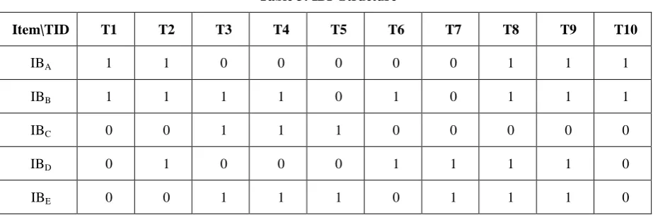
Table 3: IBP Structure

Item\TID T1 T2 T3 T4 T5 T6 T7 T8 T9 T10

IBA 1 1 0 0 0 0 0 1 1 1

IBB 1 1 1 1 0 1 0 1 1 1

IBC 0 0 1 1 1 0 0 0 0 0

IBD 0 1 0 0 0 1 1 1 1 0

IBE 0 0 1 1 1 0 1 1 1 0

The algorithm then computes Candidate1-itemset C1 which consists of items A,B,C,D,E, i.e , C1 = { A,B,C,D,E}

The support count of each itemset in C1 is computed by counting the number of 1’s in their corresponding item bit patterns. From the above table it is observed that sup(A) = 0.5, sup(B)= 0.8, sup(C) = 0.3, sup(D) = 0.5, sup(E) = 0.6.

All the itemsets in C1 satisfies ms threshold and these are placed in frequent-1 item set F1. F1= {A, B C D, E}.

The support count for each item in C2 is computed by performing bitwise AND(^) operation between corresponding bit patterns in IBP.

For example,

For item set AB, IBA ^ IBB= (1100000111) ^ (11111010111) = 1100000111.The no. of 1’s in the resultant bit vector is 5, so the sup( AB ) = 0.5. In a similar way, the support of each item set in C2 is computed and is as follows sup(AC) = 0, sup(AD) = 0.3, sup(AE) = 0.2, sup(BC) = 0.2, sup(BD) = 0.4, sup(EB) =0.4, sup(CD) = 0.1, sup(CE) = 0.3, and sup(DE) = 0.3.

Thus the frequent-2 item set is F2= {AB,AD,BD,BE,CE,DE} where the support of each itemsets is more than or equal to ms and the infrequent-2 item set is N2= {AC,AE,BC,CD} where the support count of each itemsets is less than ms. After this iteration

FS= FS U F2 i.e. FS= Ø U { AB, AD, BD, BE, CE, DE} IFS= IFS U N2 i.e. IFS= Ø U {AC, AE, BC,CD}

FS= {AB, AD, BD, BE, CE, DE} and IFS= {AC, AE, BC, CD}.

The resultant bit map of each item of F2 are stored in a new bitmap table NIBP which is shown in Table .4

Table 4: NIBP Structure

NIBAB 1 1 0 0 0 0 0 1 1 1

NIBAD 0 1 0 0 0 0 0 1 1 0

NIBBD 0 1 0 0 0 1 0 1 1 0

NIBBE 0 0 1 1 0 0 0 1 1 0

NIBCE 0 0 1 1 1 0 0 0 0 0

NIBDE 0 0 0 0 0 0 1 1 1 0

The candidate 3- item set C3 is generated by joining F2 with F1 and are placed in C3 C3= {ABC, ABD, ABE, BCD, BCE, BDE, ACE, CDE, ADE}

The support count for each item in C3 is computed by performing bitwise AND (^) operation between corresponding bit patterns in NIBP and IBP.

For example,

For item set ABD, NIBAB ^ IBD=(1100000111) ^ (0100011110)= 0100000110

The number of 1’s in the resultant bit vector is 3, so the sup (ABD) = 0.3. In a similar way the support of each itemset in C3 is computed and is as follows sup (ABC) = 0.2, sup(BCD) = 0, sup(BDE) = 0.2, sup(CDE) = 0, sup(ABE) = 0.2, sup(BCE) = 0.2, sup(ACE) = 0, sup(ADE) = 0.2.

Thus the frequent-3 item set is F3= {ABD}, as the support of itemset is more than ms and the infrequent-3 item set is N3= {ABC, ABE, BCE, BDE, ACE, CDE, ADE, BCD} as the support count of itemset is less than ms. After this iteration

IFS= IFS U N3 i.e. IFS={AC,AE,BC,CD, BC, ABE, BCE, BDE, ACE, CDE, ADE,BCD }.

The computed bit patterns of F3 are overwritten in NIBP as the previous values of NIBP are not used for further processing. In this way, memory space can be efficiently utilized. Moreover there is no need to scan the database to generate the candidate set and that can be achieved by performing the AND operation between the bit patterns.

The candidate 4- item set C4 is generated by joining F3 with F1 and are placed in C4 C4= {ABCD, ABDE}

The support count for each item in C4 is computed by performing bitwise AND (^) operation between corresponding bit patterns in NIBP and IBP. For example,

for item set ABCD, NIBABD ^ IBC = (0100000110) ^ (0011100000) = 0000000000

The number of 1’s in the resultant bit vector is 0, so the sup (ABCD) = 0.0. In a similar way support of each itemset C4 is computed and is as follows sup (ABDE) = 0.2.

Thus the frequent-4 item set is F4 = Ø and infrequent-4 item set is N4= {ABCD,ABDE} as the support count of itemset is less than ms. After this iteration

FS= FS U F4 i.e. FS = {AB, AD, BD, BE, CE, DE, ABD} IFS= IFS U N4 i.e.

IFS= {AC,AE,BC,CD,ABC,ABE,BCE,BDE,ACE,CDE,ADE,BCD, ABCD, ABDE }. Now the algorithm terminates as there are no items exist in F4.

Then PARNAR procedure is called for generating association rules by sending FS and IFS as inputs.

PARNAR procedure computes correlation between each pair of itemsets and then generate positive and negative rules. Let us consider the frequent item set AB.

CorrAB= 0.5/(0.5*0.8) = 1.25.

As correlation between A and B is greater than 1,so A and B are positively correlated and generates positive association rules A



B with confidence 1 and B



A with confidence 0.625.

Let us consider another frequent itemset BE. CorrBE= 0.4/(0.8*0.6) = 0.83.

As correlation between B and E is less than 1, though the item set BE is frequent these two are negatively correlated and generates negative association rule such as ¬B



¬E with confidence 0.6.

as correlation between A and E is greater than 1,so these two items are positively correlated and generates negative association rules ¬A



E with confidence 0.6.

In this proposed method, there is no possibility of generating contradictory rules such as ¬C



D, ¬C



¬D. This process is repeated for each itemset in FS and IFS. Finally resultant positive and negative association rules which are placed in Positive Rule Set and Negative Rule Set are given below.

PAR= {A



B, B



A, D



B, C



E, D



E, AB



D, D



AB, B



DA, A



DB, A



BD} NAR= {A



¬E, ¬A



E, B



¬C, ¬B



¬E, ¬C



B, C



¬B, C



¬D, ¬C



D, A



¬BC, ¬AB



E, AB



¬CD, ¬A



BDE, ¬AB



¬E, AB



¬C, B



¬DE}.

Then ROPNR procedure is called for generating refiltered association rules by sending PRS and NRS as inputs. ROPNR procedure computes rule strength of each rule to generate refiltered positive and negative rules.

Let us consider the rule AB



D

compute weight AB



D=[occurrence(AB)*occurence(D)]/totalnoof transactions =8*5/10

priority AB



D= weight AB



D* sup(AB U D)/(sup(AB)*sup(D)) 4*0.8*0.5=1.6>1

As priority is >1 it is considered as Refiltered positive rule Let us consider the rule B



DA

compute weight B



DA=[occurrence(B)*occurence(DA)]/totalnoof transactions =5*5/10

priority B



DA= weight B



DA* sup(B U DA)/(sup(B)*sup(DA)) 2.5*0.5*0.5=0.625<1

As priority is <1 it is not considered as Refiltered positive rule Let us consider the rule A



¬BC

priority A



¬BC = POI(A)* POI(BC)/OOi(BC)

=0.5*0.625/0.25=1.25>1 so it is considered as refilterd negative rule

This process is repeated for each rule PRSNRS. Finally resultant refiltered positive and negative association rules which are placed in RPRS and RNRS given below.

RPRS= {A



B, B



A, AB



D, A



BD}

RNRS= {A



¬E, ¬A



E, C



¬B, A



¬BC, ¬AB



E, ¬A



BDE, ¬AB



¬E, B



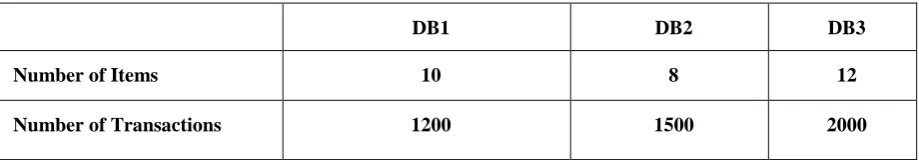
¬DE}.

Experiments are conducted on synthetic dataset to study the performance of the proposed algorithm. The three synthetic databases termed as DB1, DB2, DB3 are considered for the experiment purpose. The number of

items and the number of transactions of these databases are shown in the Table 5.

Table 5: Synthetic Databases

DB1 DB2 DB3

Number of Items 10 8 12

Number of Transactions 1200 1500 2000

The proposed algorithm is applied on the above three databases and the results are shown in the Table 5. Minimum support, minimum confidence which are considered for the experiment for each database are shown in this table. The execution time of the proposed algorithm against three databases is also shown in the Table 6.

Table 6: Minimum Support (ms)/Run time(s)

Another experiment is conducted on DB1 by proposed algorithms to show the efficiency in terms no of rules shown in Table 7.

Table 7: Number of positive and negative rules / Minimum Support (ms)

ms Number of positiverules

Number of refiltered positive rules

Number of negative rules Number of refiltered negative rules

0.1 358 153 567 432

0.3 287 204 329 280

0.5 179 104 205 109

0.7 97 52 146 100

The Table 7 shows that the proposed method is efficient in terms of rules.

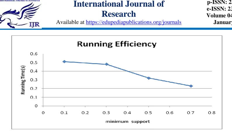
The Figure 1 illustrates the effect of minimum supports on runtime for Database DB1.

Data bases ms mc Run Time(s)

DB1 0.5 0.5 0.32

DB2 0.4 0.5 0.26

Figure 3.1: Minimum Support (ms) / Runtime

As the ms value increases, the runtime of the proposed method decreases drastically and is observed in the above graph.

The effect of number of rules by varying ms is shown in the Figure 2.

Figure 2: Minimum Support (ms) / Number of positive rules

The above figure illustrte that number of positive rules decreased when ms is incresed . The following Figure 3 illustrate the effect of ms on number of negative rules for DB1

6.CONCLUSION

In this paper, new algorithm is proposed to generate positive and negative association rules from the transactional database efficiently. A novel structure IBP (Item based bit pattern) is used to calculate support count easily, which reduces the number of database scans. Although there is flexibility of IBP, for each candidate generation phase new IBP is overwritten on the previous structure which leads to better memory utilization and increases the processing speed.

Huge number of rules can be discovered. Thus it becomes difficult for decision makers to find out the relevant rules . item based refilterization is used for relevant rules This method relies on correlation co-efficient for rule interestingness measure. The experimental results proved that the proposed algorithm is effective, efficient and promising.

REFERENCES

*1+ R.Agarwal, T.Imielinaki and A.Swami, “ Mining Association Rules between set of items in large Databases”, In Proceeding of the 1193 ACM

SIGMOD International conference on

management of data. Newyork, ACM Press, 1993, pp 207-216.

*2+ A.Savasere, E.Omiecinki and S.B.Navathe, “ An Efficient Algorithm for Mining Association Rules in large databases”, In Proceedings of the 21st international conference on very large databases. Zurich, Switzerland, 1995, pp 432-444.

*3+ J.Han, J.Pei, and Y.Yin, “ Mining Frequent Patterns without Candidate Generation”, In Proceedings of ACM SIGMOD International conference on management of data. May 2000, pp 486-493.

*4+ R.Srikant and R.Agarwal, “ Mining Generalized

Association rules”, VLDB Zurich,

Switzerland,1995, pp407-419.

*5+ Brin.S, Motwani.R and silverstein.C, “ Beyond Market Baskets: Generalizing Association Rules to Correlation”, In Proceeding of the ACM SIGMOD conference 1997, pp 265-276.

[6]. A.Savasere, E.Omiecinski, and S.Navathe, “ Mining for Strong Negative Association in Large Database of Customer Transactions”, In Proceedings of the ICDE 1998, pp 494-502. *7+ H.zhu, Zhang, Xu,“ An Effective Algorithm for Mining Positive and Negative Association Rules”, In Proceedings of the International conference on computer science and software engineering 2008, pp 623-629.

*8+ X. Wu, C. Zhang, and S. Zhang, “ Mining Both Positive and Negative Association Rules”, In Proceedings of 19th International Conference on

Machine Learning 2002, Sydney, Australia, pp 658-665.

*9+ Dong,X, Wang.S, Song. H, “ Study of Negative Association Rules”, Beijing institute of Technology Journal, 2004, pp 978-981.

*10+ Dong.X, Sun.F, Han.X. Hou.R, “ Study of Positive and Negative Association Rules based on Multi confidence and Chisquared Test”, LNAI 4093, Springer2006, Heidelberg, pp100-109. *11+ Yuan,X, Buckles,B.P, Yuan,Z, Zhang, J, “ Mining Negative Association Rules ”, In Proceedings of the seventh International

Symposium on Computers and

Communications(ICSS 2002),IEEE Computer

Socity,Washington DC, pp 623-631.