Search for Higgs Boson Production Beyond the Standard Model Using the Razor Kinematic Variables in pp Collisions at √s=8 TeV and Optimization of Higgs Boson Identification Using a Quantum Annealer

(1)

Standard Model Using the Razor Kinematic

Variables in pp Collisions at

√

s

=

8 TeV

and

Optimization of Higgs Boson Identification Using

a Quantum Annealer

Thesis by

Alexander Mott

In Partial Fulfillment of the Requirements

for the Degree of

Doctor of Philosophy

California Institute of Technology

Pasadena, California

2015

(2)

(3)

Acknowledgments

I would like to thank my PhD advisor, Maria Spiropulu, for all of her support, advice,

and guidance over the course of my graduate studies. She has been an incredible

mentor and her passion and enthusiasm for experimental physics have made it a

pleasure as well as a privilege to work with her. I would also like to Harvey Newman

for his insightful and valuable help and insight.

I would like to thank Massimiliano Chiorboli, who helped me get started on my

very first project on CMS; Adi Bornheim, who helped me learn about the Higgs to

two photon analysis; and Maurizio Pierini, whose support and deep knowledge of

particle physics have been extremely helpful in many different projects.

I would like to thank Daniel Lidar and Josh Job for their help in all stages of

the quantum annealer project. Their support and insight made that entire project

possible.

Finally, I would like to thank my parents, Anne and Geoffrey, and my brother

Christian. Without their support and encouragement I never would have been able

(4)

(5)

Abstract

In the first part of this thesis we search for beyond the Standard Model physics

through the search for anomalous production of the Higgs boson using the razor

kinematic variables. We search for anomalous Higgs boson production using

proton-proton collisions at center of mass energy√s= 8 TeV collected by the Compact Muon

Solenoid experiment at the Large Hadron Collider corresponding to an integrated

luminosity of 19.8 fb−1.

In the second part we present a novel method for using a quantum annealer to train

a classifier to recognize events containing a Higgs boson decaying to two photons. We

train that classifier using simulated proton-proton collisions at√s= 8 TeV producing

either a Standard Model Higgs boson decaying to two photons or a non-resonant

Standard Model process that produces a two photon final state.

The production mechanisms of the Higgs boson are precisely predicted by the

Standard Model based on its association with the mechanism of electroweak

sym-metry breaking. We measure the yield of Higgs bosons decaying to two photons in

kinematic regions predicted to have very little contribution from a Standard Model

Higgs boson and search for an excess of events, which would be evidence of either

non-standard production or non-standard properties of the Higgs boson. We divide

the events into disjoint categories based on kinematic properties and the presence of

additional b-quarks produced in the collisions. In each of these disjoint categories, we

use the razor kinematic variables to characterize events with topological

configura-tions incompatible with typical configuraconfigura-tions found from standard model production

of the Higgs boson.

(6)

the Higgs boson mass and localized in a small region of the razor plane. We observe

5 events with a predicted background of 0.54±0.28(syst.), which observation has a

p-value of 10−3 and a local significance of 3.35σ. This background prediction comes

from 0.48 predicted non-resonant background events and 0.07 predicted SM higgs

boson events. We proceed to investigate the properties of this excess, finding that

it provides a very compelling peak in the di-photon invariant mass distribution and

is physically separated in the razor plane from predicted background. Using another

method of measuring the background and significance of the excess, we find a 2.5σ

deviation from the Standard Model hypothesis over a broader range of the razor

plane.

In the second part of the thesis we transform the problem of training a classifier

to distinguish events with a Higgs boson decaying to two photons from events with

other sources of photon pairs into the Hamiltonian of a spin system, the ground state

of which is the best classifier. We then use a quantum annealer to find the ground

state of this Hamiltonian and train the classifier. We find that we are able to do this

successfully in less than 400 annealing runs for a problem of median difficulty at the

largest problem size considered. The networks trained in this manner exhibit good

classification performance, competitive with the more complicated machine learning

techniques, and are highly resistant to overtraining. We also find that the nature

of the training gives access to additional solutions that can be used to improve the

(7)

quan-tum annealer

165

7 Introduction 167

8 Quantum Annealing 171

8.1 Simulated Annealing . . . 171

8.2 Quantum Annealing . . . 172

9 Experimental Setup 179 9.1 Encoding the Problem . . . 179

9.2 Embedding the Problem on the Chimera Graph . . . 183

9.3 Practical Implementation of the Embedding . . . 187

9.4 The D-Wave 2TM Machine . . . 190

9.5 Training Sample . . . 193

10 Results 199 10.1 Network Training Results . . . 200

10.1.1 Mapping Physical Chains to Logical Nodes . . . 200

10.1.2 Solution Accuracy . . . 202

10.2 Performances of the Network in Classifying Signal Events . . . 205

10.3 Improving Success Probability and Performance . . . 209

10.4 Current Status and Outlook . . . 212

(11)

Part I

Search for Higgs boson production

beyond the Standard Model using

the Razor kinematic variables in

(12)

(13)

Chapter 1

Introduction

In A short history of nearly everything, Bill Bryson said [1]:

Physics is really nothing more than a search for ultimate simplicity,

but so far all we have is a kind of elegant messiness.

In particle physics, this elegant messiness is known as the Standard Model (SM),

which aims to understand the most fundamental building blocks of nature. The SM

is one of the most successful theories in the history of science and has accurately and

precisely described practically every experimental result obtained over the last few

decades at the relevant scales [2]. It has also had success at predicting the presence

of subsequently observed particles such as a wide variety of mesons, the top quark,

and the Higgs boson.

Despite all this success, the SM doesn’t conquer every experimental challenge. It

doesn’t explain the mass of neutrinos required by the observation of neutrino

oscilla-tions; it doesn’t explain dark matter or dark energy; it doesn’t reconcile with general

relativity or explain why the gravitational and electroweak scales are so far apart;

and it doesn’t explain the matter-antimatter asymmetry observed in the universe. It

also takes quite a lot of parameters as input and thus mostly can’t explain why the

particles have the masses they do (the Higgs mechanism does predict masses of some

particles based on other observables). It also doesn’t explain why (or if) there are

exactly three generations of fermions.

This thesis attempts to address some of these challenges by looking for beyond the

(14)

experi-mental evidence for the deeper theory of nature: Bryson’s “ultimate simplicity.” The

production of the Higgs boson is very precisely predicted by the standard model based

on its vacuum expectation value and the masses of the fermions, so any anomalous

production is strong evidence for physics not predicted by the SM. We consider this

from the point of view of the production of supersymmetric particles that decay into

(among other things) Higgs bosons but we aim to keep this as general as possible to

allow for other interpretations. We use the di-photon decays of the Higgs boson to

perform our search, since this channel gives a very clean experimental signature and

still has a sufficiently high branching ratio to allow a large sample of decays to this

final state.

In Chapter 2 we give an overview of the portions of theory of the standard model

and supersymmetry relevant to this study. Entire theses can and have been written

on each of these theories so we restrict ourselves only to the key points relevant to

our experimental search. We discuss the particle component of the SM and how the

forces arise through preserved local symmetries of the theory. We discuss the recently

discovered Higgs boson, its theoretical origins, its properties, and the problem of

the divergence of the radiative corrections to its mass. We then discuss how this

problem can be solved through the introduction of a new supersymmetry, mostly in

the context of the minimal supersymmetric standard model. This model has a large

number of degrees of freedom, so we discuss the simplifications made to make some

of its predictions experimentally testable while retaining its key attributes.

In Chapter 3 we discuss the Large Hadron Collider (LHC) and the Compact

Muon Solenoid (CMS) detector. This analysis uses 19.8 fb−1 of data from

proton-proton collisions recorded by the CMS detector during the 2012 run of the LHC

taken at √s = 8 TeV. We describe the various subdetectors of CMS used to measure

different attributes of the particles produced by the collisions and discuss how the

raw measurements made by the detectors are built into detector-level quantities.

In Chapter 4 we discuss how the detector-level quantities are transformed into

measurements of the energy and momentum of particles produced in the collisions.

(15)

focus paid to the method of reconstructing and identifying photons and jets. We

discuss the multivariate methods used to provide excellent estimation of the energy

of photons used in the event, which is of vital important when working in theH →γγ

channel. We also discuss the measurement of missing energy from the detector energy

deposits, which can be used to gain some information about particles escaping from

the detector.

In Chapter 5 we present the analysis used to search for anomalous production of

the Higgs boson. We describe the blinding procedure that prevents us from looking

in the signal region before freezing the analysis and the method of estimating the

backgrounds using data-driven and Monte Carlo (MC) techniques. We discuss the

kinematic variables, known as therazor variables, used to acheive excellent sensitivity

to kinematic configurations indicative of beyond the standard model processes and

used to cut away standard model background.

In Chapter 6 we unblind the analysis and show the results of the search. We

present both the results of the main analysis and a cross-check analysis designed

to measure background in a different way to ensure that we are not biased by our

method. We observe an excess of events in a signal sensitive region and proceed to

analyze and characterize this excess. While the excess has a moderate significance,

it is a small absolute number of events, so characterization cannot be performed in a

compelling way. We conclude by looking forward to the next run of the LHC, where

(16)

(17)

Chapter 2

Theory

2.1

The Standard Model

The Standard Model (SM) of particle physics is our best current description of the

interactions between all known elementary particles. It includes spin-1_⁄₂ _fermions

that make up matter and obey the Pauli exclusion principle, spin-1 bosons that

mediate forces between these fermions, and the spin-0 Higgs boson that “gives mass”

to elementary particles. The fermions are divided into leptons (Table 2.1) and quarks

(Table 2.2). The bosons are summarized in Table 2.3.

Name Symbol Charge Mass (GeV)

electron e− -1 5.11×10−4±1.1×10−11

muon µ− -1 0.11±3.5×10−9

tau τ− -1 1.78±1.6×10−4

electron neutrino νe 0 <2×10−9

muon neutrino µµ 0 <2×10−4

tau neutrino µτ 0 <0.02

Table 2.1: The properties of the leptons in the SM. (source: PDG [3])

Mathematically, the SM is a gauge theory defined by a Lagrangian L involving

fields. The Lagrangian of the SM is the most general renormalizable expression

respecting a set of symmetries. These symmetries are given by a gauge group, the

action of whose members leave the lagrangian invariant. The Lagrangian is required

to respect these symmetries not only globally, but locally as well. The promotion of

(18)

Name Symbol Charge Mass (GeV)

up u +2_⁄₃ ₂_.₃0.7

−0.5×10−3

charm c +2_⁄₃ ₁_.₃_±₀_.₀₂₅

top t +2_⁄

3 173±0.51±0.71

down d -1_⁄₃ ₄_.₈+0.5

−0.3×10

−3

strange s -1_⁄

3 0.095±0.005

bottom b -1_⁄₃ ₄_.₁₈_±₀_.₀₃

Table 2.2: The properties of the quarks in the SM. (source: PDG [3])

Name Symbol Charge Mass (GeV) Spin

photon γ 0 0 1

W-boson W± ±1 80.4±0.015 1

Z-boson Z0 ₀ ₉₁_.₂_±₀_.₀₀₂₁ ₁

gluon g 0 0 1

Higgs boson H 0 125.7±0.4 0

Table 2.3: The properties of the bosons in the SM. Charge represents EM charge only and central values for the masses are quoted. (source: PDG [3])

of a bosonic field to form a gauge covariant derivative. This field can be interpreted

as a force between different points in space-time and the quantization of this field is

interpreted as the force carrier [4].

Each interaction in the SM is associated with an interaction strength α. A

con-sequence of the renormalizability of the theory is that these strengths will change, or

“run,” with the energy of the interaction. The way in which the coupling constants

run is dependent on the group structure and form factors of the symmetry group

governing the interaction and corresponding form factors.

The interactions of the standard model particles under the electromagnetic

in-teraction can be described by quantum electrodynamics (QED), which is a gauge

theory based on a U(1)em symmetry group [4]. Promoting this global symmetry to a

local symmetry requires that the lagrangian be invariant under space-time dependent

complex phase changes

ψ(x)→eiα(x)ψ(x)

which requires the introduction of a spin-1 massless gauage boson, the photon.

(19)

Higgs field, which will be discussed further in section 2.1.1.

In addition to their electromagnetic interactions, the quarks also interact via the

strong force. The gauge theory of the strong force, called quantum chromodynamics

(QCD), is based on the SU(3)C symmetry group [5, 6]. The quarks carry a charge

under this symmetry, known as color charge, which is selected from one of three

charges (red, green, and blue). Promoting the SU(3) symmetry to a local symmetry

introduces a massless spin-1 boson that mediates this force, known as the gluon.

Unlike in QED, where the photon is neutral, the gluon carries color charge with two

separate colors allowing differently charged quarks to interact. There are 8 gluons

with different combinations of color index corresponding to the the 8 generators of

the adjoint representation of SU(3).

The structure of the field strength tensor for the gluon gives rise to a phenomenon

known as asymptotic freedom, where the strong force weakens between particles at

high energies. Over short distances, colored particles behave like free particles, while

as distances increase the strength of the strong force increases. If two colored particles

get too far apart, there is eventually so much energy in the gluon field between them

that it is energetically favorable to create a new quark-antiquark pair. If a colored

particle is produced with a large momentum, as in LHC collisions, this process will

be repeated many times, creating a large number of color neutral baryons travelling

in the direction of the initial particle. This process is known as hadronization and

forms what we call a jet.

The final component of the SM is the weak interaction, which is based on an

SU(2)L×U(1)Y symmetry group. Gauging this group produces 4 massless spin-1

gauge bosons (in fact, the U(1)em group of the electromagnetic force is actually a

subgroup of this interaction and the gauging of this full electroweak theory produces

the photon), and the mixing of these produces theW± and Z0 bosons. These bosons

are massless in the basic electroweak theory and acquire mass through the Higgs

(20)

2.1.1

The Higgs Mechanism

The Higgs mechanism is a process of adding an additional SU(2) doublet of

spin-0 fields (φ) to the electroweak lagrangian, which produces electroweak symmetry

breaking (EWSB) [7–11]. This field is assigned a quadratic potential

V(φ) = −µ2φ†φ+λ 2(φ

†

φ)2

with λ, µ2 _∈

R and µ2 >0. This potential has a degenerate ground state where the

Higgs field acquires a nonzero vacuum expectation value (VEV) v = pµ2

/λ due to

the requirement that µ2 _> _{0. This VEV breaks the} _SU₍₂₎

L ×U(1)Y electroweak

symmetry.

One combination of generators ofSU(2)L×U(1)Y leaves the VEV invariant, which

leaves the boson massless. This combination producesU(1)emand the electromagnetic

theory. The other combinations of generators acquire additional longitudinal degrees

of freedom and gain mass, and produces the W± and Z0 _{bosons. One neutral scalar}

field from the Higgs doublet is left and is associated with the Higgs boson. This

boson in turn gives mass to the fermions through Yukawa couplings. The Higgs

boson acquires a mass from the VEV equal to mH =

√

2λv. The parameters µ2 _and

λ are not set by the theory, but CMS and ATLAS have measured mH = 125.7±0.4

GeV [3].

2.1.2

SM Higgs Boson Production Modes

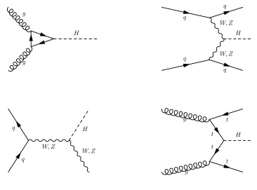
At √s = 8 TeV, there are four major production modes to produce a Higgs boson

in pp collisions, shown in Figure 2.1 [12]. For mH = 125 GeV, the SM cross sections

and expected number of total events to be produced in the 2012 CMS dataset can be

seen in Table 2.4.

The different production modes are associated with different kinematics and final

states for the events containing the Higgs boson. Additional objects may be produced

(21)

final state radiation of one of the produced objects. These processes are simulated

using PYTHIA 6 [13] and POWHEG [14–18] and use GEANT 4 [19] to simulate

iteraction with the detector.

g g

H

q q

q W, Z W, Z

q

H

q q

W, Z

W, Z H

g

g _t

t t

t

H

Figure 2.1: The four production modes of the SM Higgs boson accessible in the LHC with √s = 8 TeV and R Ldt = 19.8 fb−1. They are called gluon fusion (top left), vector boson fusion (top right), vector boson associated production (bottom left) and top associated production (bottom right).

2.2

Supersymmetry

While the Higgs mechanism provides an elegant solution to the problem of electroweak

symmetry breaking, it introduces at least one additional problem: the mass of the

higgs boson receives enormous quantum corrections from every particle that couples

(22)

Process Name Process Cross-section (pb) Expected Events in 19.8fb−1

Gluon Fusion pp→H 19.27 869.9

Vector Boson Fusion pp→qqH 1.578 71.2

Associated Production pp→V H 1.1199 50.6

Top Associated Production pp→ttH 0.1293 5.8

Total 22.1 997.6

Table 2.4: The SM Higgs boson production mechanisms considered as background to this analysis. The cross-sections are for 8 TeV pp collisions withmH = 125 GeV. To

get the expected events, we useBr(H →γγ) = 2.28×10−3. Cross-sections are taken from [12].

a one loop quantum correction to its mass of

∆mH =−

|λf|2

8π2 Λ 2

U V +· · ·

where λf is the strength of the coupling (|λtop| ≈1), ΛU V is the scale at which new

physics enters and cuts off the loop intergral, and the higher order terms go at most

with log(ΛU V). If we consider the coupling to a scalar, we instead get contributions

of the form

∆mH =

λS

16π2[Λ 2

U V +m

2

Slog(ΛU V/mS) +· · ·]

If we believe that the SM is the full theory, then we must take ΛU V ≈ MP lanck

where quantum gravity becomes important. This provides a value of mH 30 orders

of magnitude incompatible with the measured value [20–22].

One solution is to invent new physics at a lower scale so the ΛU V is lower; however,

this still raises issues if they couple even indirectly to the Higgs boson. A more

robust solution is to cancel the divergences in ∆mH by a symmetry. We notice that

the contributions from fermions and scalars have opposite sign, so if each fermion

in the standard model is accompanied by two complex scalars with λS = |λf|2 then

the quadratic divergences can cancel. Since there are no candidates for this pairing

within the standard model, a new symmetry between fermions and bosons called

supersymmetry (SUSY) is posited [23].

There are many possible models that implement this posibility, but the simplest is

(23)

standard model (MSSM). We form chiral supermultiplets pairing each standard model

fermion with its supersymmetric partner. Since the left-handed and right-handed

components of the fermions have different gauge transformation properties in the

SM, each must have its own complex scalar partner (hence we achieve the required 2

SUSY particles for each fermion). The scalar partners of the fermions are known as

sfermions (squarks, sleptons, etc.) and are usually denoted with a tilde (˜q, ˜l, etc.).

The vector bosons are associated with spin-1_/₂_{fermionic superpartners, referred to}

as gauginos and placed in gauge supermultiplets. Before EWSB, theSU(2)L×U(1)Y

symmetry of the EW gauge is associated with 4 vector bosons: W±, W0, and B0,

each of which has its own fermionic superpartner denoted with a ˜ (e.g. ˜W±). After

EWSB, just as the SM W0 and B0 mix to give the Z and γ, the ˜W0 and ˜B0 mix

to give ˜Z and ˜γ. Taken together with the Higgsinos (also spin-1_/₂_{), these sparticles}

can mix to form 2 mass eigenstates which we call neutralinosχ0_i₌₁_,₂; the charged ˜W±

states can also mix to form 2 charginosχ±_i₌₁_,₂. In many models, the lightest neutralino

(written χ0₁ or, more commonly, χ0) is the lightest supersymmetric particle.

Supersymmetry does not independently preserve baryon and lepton number, which

leaves it open to predicting proton decay and lifetimes incompatible with the

obser-vation of the lifetime of the universe and lower limits on the proton lifetime. One

way to avoid this is to introduce a quantity known as R-parity

R ≡(−1)2s+3(B−L)

that is conserved by supersymmetry (sis the spin of the field). It can either be added

in an ad-hoc way, or it can be added as part of a model that conserves R-parity

automatically [24]. By construction, R=+1 for all SM particles and R=-1 for all

SUSY particles. The introduction of this conserved quantity inplies that there are

always an even number of SUSY particles in any interaction, which has important

phenomenological consequences:

SUSY particles must be pair produced at the LHC

(24)

well as an arbitrary number of SM particles

the lightest supersymmetric particle (LSP) is stable

The third point follows as consequence of the second (the lightest particle has no valid

R-parity preserving decays). This implies that a weak scale LSP could potentially be

a candidate for a particle explanation of dark matter. It also means the LSPs would

escape the CMS detector undetected.

Since this whole discussion began by introducing SUSY to cancel divergences in

the Higgs boson mass, it is no surprise that massive SUSY particles couple to the SM

Higgs boson. This means that the decays ˜q→Hχ0 andχ2 →Hχ0 should be allowed

when there is enough mass splitting between the particles to allow it. So far, SUSY

has eluded all attempts to find it, but these decays, coupled with the measurement

of the mass of (a) Higgs boson, offer a promising new channel.

2.2.1

Simplified Models

If supersymmetry is realized in nature it must be a broken symmetry, since sparticle

states with identical masses to their SM partners have been excluded by previous

experiments. This implies that there must be supersymmetry violating terms in the

SUSY Lagrangian; in order to avoid adding additional ultraviolet divergences, this

breaking should be soft. With all the soft terms added, SUSY adds several hundred

new masses, mixing angles and phases to the model.

Since a model with several hundred parameters is difficult to work with when

pre-senting experimental results, we often interpret our results in the context of simplified

models that make the asumption that only a few states have masses that are

accessi-ble at the LHC [25]. In particular, in this work, we focus on a model where only the

neutralinos and charginos are accessable at the LHC, with the lightest neutralino ˜χ0 1

(25)

decays to consider are

˜

χ₂0 →Hχ˜0₁ χ˜0₂ →Zχ˜0₁

˜

χ₂0 →W±χ˜∓₁ χ˜±₁ →W±χ˜0₁

If we assume that the χ0

2 and χ

±

1 are nearly degenerate (we drop the ˜χ notation

for convenience), then the 3rd decay is through a virtual W∗, which decays to low

momentum particles. In an R-parity conserving model, the phenomenology of these

decay channels is a set of final states with either two vector bosons, two Higgs bosons,

or a vector boson and a Higgs boson, all with two additional neutralinos that escape

the detector [26]. If we consider only models where the mass splitting between the

NLSP and LSP is ∆m _& 130 GeV, then all of these bosons would be on-shell. Of

course there are other potential decay channels for the neutralinos and charginos that

may or may not be allowed or dominant in different regions of parameter space, but

we focus on cases where the decays listed are most important.

From an experimental point of view, final states including a Higgs boson have

some attractive properties that can be exploited to increase the sensitivity to these

models. The Higgs boson has a much smaller width than the Z or W (≈4 MeV versus

2.1 and 2.5 GeV respectively), so in a real experiment the observed width is just the

resolution of the detector and the major production modes are straightforward to

model. Its decay into photons gives it a very clean experimental signature, and its

relatively small standard model cross section means it is quite easy to find kinematic

regions with virtually no predicted Higgs boson events without going onto the tails

of the distributions. In this study, therefore, we focus only on decays that produce a

Higgs boson.

Figure 2.2 shows the diagrams of the simplified model that we study here. We

require at least one leg to have the χ2 → Hχ1 decay and allow the other leg to

decay as it will. We have already said that we take the χ±₁ and the χ2 to be near

degenerate, so we are left with only two more parameters to consider: the mass of the

(26)

(27)

(GeV)

2

χ

m

150

200

250

300

350

400

450

500

550

Cross-section (pb)

-2

10

-1

10

1

10

±

1

χ

2

χ →

pp

2

χ

2

χ →

pp

Figure 2.3: The production cross section for neutralino-neutralino and chargino-neutralino production as a function of the mass in the simplified model under consid-eration for pp collisions at√s = 8 TeV.

the decays of the Higgs boson to two photons, so we account for the branching ratio

(0.0028 at mH = 125 GeV) so we can calculate that we expect to see one event for

a model with a cross-section of σ = 0.04 pb with an acceptance of 50%. Based on

the scaling of the cross section, we only consider models with mχ2 <200 GeV, which

would produce at least a few events under realistic acceptance. We can therefore

define the set of models that are guiding this analysis as those shown in Figure 2.2

(28)

(29)

Chapter 3

Experimental Setup

3.1

The Large Hadron Collider

The Large Hadron Collider (LHC) is a superconducting hadron collider located at

CERN near Geneva, Switzerland [29]. It occupies a 26.7 km circumference tunnel

that lies between 45 m and 170 m below the surface originally built for the LEP

ex-periments. It is designed to provide collisions between two beams of protons traveling

in opposite directions within the ring each with an energy of 7 TeV at a peak

instanta-neous luminosity of 1034cm−2s−1. Thus far, the machine has achieved 8 TeV collisions

(4 TeV in each beam) and a peak luminosity nearing 7.7×1033_cm−2_s−1 _[30].

The beams are divided into clusters of protons, called bunches, within the machine.

The LHC is designed to operate with a 25 ns spacing between the bunches and a

total of 2,808 bunches, each containing 1.15×1011protons, within the ring. Thus far

only a spacing of 50 ns between the bunches has been achieved with a peak of 1380

bunches circulating. The bunch charges have been higher than design, with a peak

of 1.6×1011 _{protons per bunch achieved.}

The beam circulates in two parallel rings where the bunches are bent using

su-perconducting dipole magnets. For cost and space reasons, the two counter-rotating

beams are housed in adjacent beam tubes within the same cryostat. Since the beams

have the same charge, they each require a magnetic field pointing in the opposite

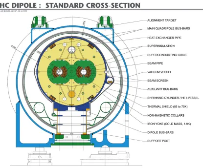
direction to stay within the ring. Dipole magnets are used to achieve this, producing

(30)

shown in Figure 3.1.

Figure 3.1: Schematic cross section of an LHC dipole magnet.

The dipole magnets are NbTi superconductors maintained at 2 K by a cryostat.

They are capable of producing a field of up to 8 T, with the exact strength set

depending on the energy of the protons within the machine. The LHC rings contain

1,232 of these magnets.

3.1.1

Collisions and Pileup

As mentioned before, the peak luminosity achieved in 2012 has beenL= 7.7×1033 cm−2s−1

divided into 1380 bunches separated by 50 ns. For most of the length of the ring, the

two beams counterrotate in separate parallel beampipes. To produce collisions, the

two beams are steered into a single beampipe and pass through each other at 8

(31)

where some protons from one bunch collide with other protons from the other bunch.

One can calculate the peak expected number of collisions per crossing from the peak

luminosity ( = 7.7×1033_cm−2_s−1 _{per bunch), the total proton-proton cross section}

at√s= 8 TeV (σpp= 101.7 = 101.7×10−27cm2, measured by TOTEM [31]) and the

bunch spacing (n= 5.0×10−8s):

< I >=L ∗σpp∗n= 39.1 (3.1)

So in each bunch crossing, we expect about 39 individual proton-proton interactions

at peak luminosity. We are only interested in a very tiny fraction of the collisions that

are produced, but each time one collision in the bunch crossing produces a particle of

interest (a Higgs boson, for example), we will also record all the particles produced by

the other collisions in the same bunch crossing. We call these interactions “pileup”

and dealing with it is one of the largest challenges for any analysis at the LHC.

We describe in Section 3.2.2.2 how we determine which vertex produced particles of

interest (the primary vertex) and in Section 4.3.1 how we identify and remove the

energy from particles produced by these pileup interactions from the reconstruction

of the particles produced by the interaction at the primary vertex.

3.2

The Compact Muon Solenoid

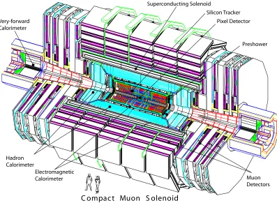
The Compact Muon Solenoid (CMS) is one of two general purpose detectors at the

LHC [32] [33]. A schematic outline is shown in Figure 3.2, showing all the major

components. CMS is designed to accurately measure all charged and neutral

par-ticles produced by a proton-proton collision using a series of different components

or sub-detectors, each specialized at measuring specific attributes of products from

the collision. At its core is the eponymous superconducting solenoid that produces a

3.8 T magnetic providing large bending power to enable precise determination of the

momentum of charged particles. The detector is divided into 4 main subdetectors:

(32)

electromagnetic calorimeter (ECAL), for measuring the shower from electrons and

photons; the hadron calorimeter (HCAL), for measuring the shower from hadrons;

and the muon systems, for measuring the energy and momentum of muons.

We define a coordinate system that will be used consistently when talking about

positions of subdetectors and particles with the (0,0,0) point at the center of the

detector. The ˆx direction points toward the center of the LHC ring from the center

and the ˆy direction points upward toward the surface. The ˆz direction, then, points

along the beamline to the left side of the detector (toward the Jura mountains) to

make a right-handed coordinate system. Azimuthal angle (φ) is measured in the x-y

plane from the x axis while polar angle is measured from the z axis. We will frequently

use the variable psuedorapidity, which is defined as

η=−ln

tan

θ

2

We call a vector “transverse” to the beamline if~v·zˆ= 0 (i.e.,~v lies in the x-y plane).

The detector is divided into three major regions: the barrel, covering the central

(low η) part of the detector transverse to the beamline; the endcaps, covering the

intermediate (middle η) regions; and the forward regions, covering the very forward

(high η) region where particles from the interaction emerge nearly parallel to the

beamline.

3.2.1

The CMS Solenoid

The CMS solenoid is shaped like a hollow cylinder centered around the beamline,

with an internal diameter of 6 m and a length of 12.5 m [34] [35]. It is a

supercon-ducting magnet designed around a 4 layer NbTi coil to produce a 4 T magnetic field

within the hollow bore; at full current, the solenoid has a stored energy of 2.6 GJ. The

total cold mass of the solenoid is 220 T, giving a relatively high Energy/Mass ratio

of 11.6 KJ/kg, causing a large (0.15%) mechanical deformation of the solenoid

dur-ing energizdur-ing, significantly larger than the deformations found for previous detector

(33)

C ompact Muon S olenoid

Pixel Detector Silicon Tracker Very-forward

Calorimeter

Electromagnetic Calorimeter Hadron

Calorimeter

Preshower

Muon Detectors Superconducting Solenoid

Figure 3.2: Schematic overview of the CMS detector.

The solenoid is situated within an 10,000 T iron return yoke consisting of 3 distinct

layers divided into 7 regions (5 wheels in the central region and 2 endcap regions). A

picture of the return yoke under construction can be seen in Figure 3.3. The solenoid

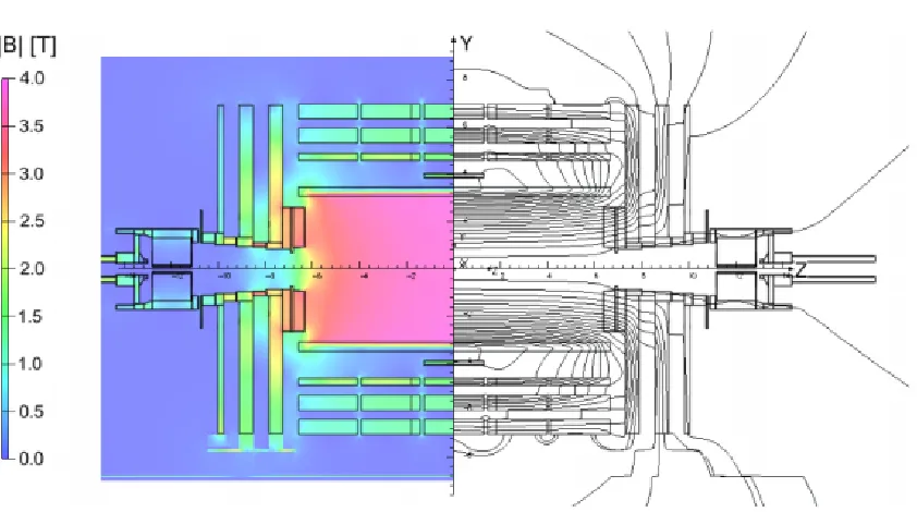
produces a significant field outside the bore and the iron yoke guides the return field

back along distinct channels (see Figure 3.4), allowing muon chambers to be placed

outside the solenoid for muon identification and measurement.

3.2.2

The CMS Tracker

The CMS tracker is designed to measure the trajectory of individual charged

parti-cles produced in an interaction as they bend in the magnetic field produced by the

solenoid. At 50 ns bunch spacing, each bunch crossing produces up to 40 interactions

(see Section 3.1.1), which altogether produce around 2000 charged particles [33]. The

(34)

Figure 3.3: The assembly of the yoke.

and 2 disks in the endcap region and a silicon strip tracker with 10 layers in the

barrel region and 3+9 disks in the endcap region [36]; the configuration can be seen

in Figure 3.5.

The three cylindrical layers of the pixel detector are situated at radii of 4.4, 7.3,

and 10.2 cm from the beamline. The two disks extend from≈6 to 15 cm in the radial

direction and are located at z = ±34.5 cm and z = ±46.5 cm from the interaction

point. Together, these cover the pseudorapidity range −2.5< η <2.5. The barrel

pixels consist of 48 million channels while the endcap disks consist of 18 million

channels each. Each channel has dimensions 100 × 150µm2, which allows the total

occupancy of the pixels to be kept very low (≈10−4) even with the very high particle

multiplicities expected at design luminosity. The placement of the barrel and pixel

layers allows almost the entire region between −2.5< η <2.5 to be covered by at

least 3 layers of pixels (see Figure 3.6).

(35)

de-Figure 3.4: Schematic view of the CMS detector with the magnetic field strength shown (left half, color Z axis) and the magnetic field lines shown (right half). One sees the magnetic field is strong and uniform inside the solenoid, while outside the solenoid it is concentrated inside the iron return yokes, which guide the magnetic field lines.

tectors with a typical cell size of 10 cm×80µm in the inner strips (tracker inner barrel

or TIB, and tracker inner disks or TID: 20 cm< r <55 cm) and 25 cm×180 µm

in the outer strips (tracker outer barrel or TOB, and tracker endcpas or TEC:

55 cm<r<110 cm). The increased distance from the interaction point keeps the

occupancy manageable despite the larger size of the strip detectors (2-3% in the

inner strips and ≈ 1% in the outer strips). There are a total of 9.6 million strip

de-tectors arranged in 15148 detector modules covering a total area of over 200 m2_{. The}

inner tracker (TIB/TID) provides up to 4r−φ measurements on a given trajectory.

The TOB provides another 6 r−φ while the TEC provides up to 9φ measurements

per trajectory. The individual measurements from the layers of the pixel and

sili-con trackers are used by the track resili-construction to resili-construct the trajectories of

particles moving through the tracker.

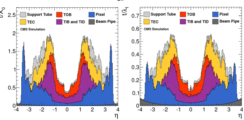
The material budget for the tracker is shown in Figure 3.7. One sees that in the

very central region|η|<1, the tracker is very “thin” (less than one radiation length

(36)

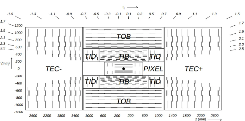
Figure 3.5: The layout of the subdetectors within the CMS tracker. The three barrel and two endcap layers of the pixel detector are shown in the box around the interaction region (the solid dot in the middle). The silicon tracker is divided into Tracker Inner Barrel (TIB) and Tracker Outer Barrel (TOB) layers covering the barrel and Tracker

Inner Disks (TID) and Tracker EndCaps (TEC±) covering the endcaps. From [32]

it is comparatively thick. This will play an important role in our reconstruction of

photons and electrons, which is discussed in Section 4.2.

3.2.2.1 Track Reconstruction

We reconstruct the path of charged particles through the CMS tracker using the hits

measured by the pixel and strip detectors and the equations of motion for charged

particles moving in the homogeneous magnetic field produced by the CMS solenoid.

From a given seed, the definition of which is discussed below, an initial trajectory

is estimated from the best fit to those points in 3D space, varying the kinematics of

the potential charged particle. In an iterative procedure, more hits are added to the

trajectory, to further refine the estimation until all hits are accounted for.

The iterative algorithm used to find tracks is known as the Combinatorial Track

Finder (CTF) [37]. The collection of reconstructed tracks is produced by multiple

applications (iterations) of the CTF algorithm. The aim is to find the easiest tracks

(37)

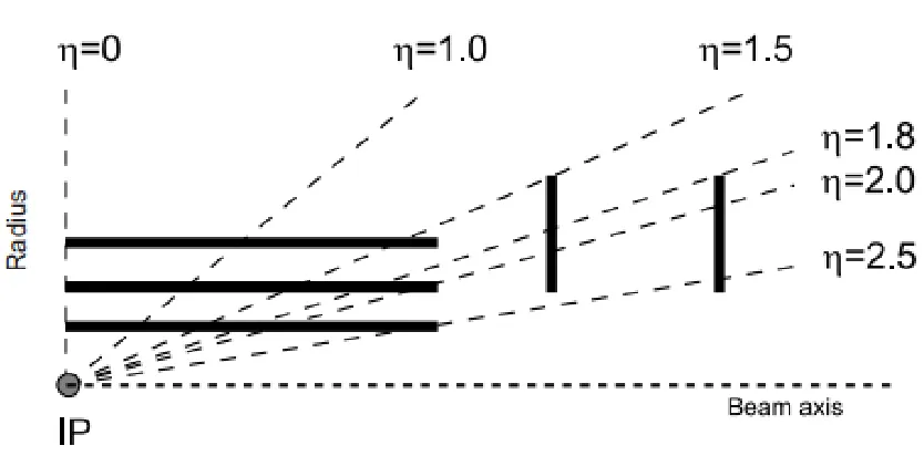
Figure 3.6: The coverage of the pixel detector. One can see that almost the entire region between −2.5 < η < 2.5 is covered by 3 layers of pixels, with a small region near the edge of the coverage only covered by the innermost barrel layer and the outermost endcap disk.

associated with these tracks, and then move on to progressively harder to find tracks

(lower pT or displaced from the interaction region) with the smaller hit collection

reducing the computational challenge at each step. The algorithm uses 6 iterations:

iterations 0-2 are designed to find prompt tracks with successively lower pT or track

quality, while iterations 3-5 are designed to find tracks originating outside of the main

interaction region.

In addition to the hits recorded by the tracker, the track reconstruction algorithm

uses information about the beam spot, which is a measurement of the average

inter-action location over many events within a given period of collisions. This serves as an

initial estimate for the interaction location for each event. Additionally, initial

per-event vertex information is reconstructed from triplets of hits in successive layers of

the pixel detectors (pixel tracks), which are extrapolated back to the interaction region

to form pixel vertices (in a manner analogous to that described in Section 3.2.2.2).

This provides a fast estimation of the locations of the primary vertices of the event,

which are then used to fit the full tracks.

(38)

Figure 3.7: The tracker material budget as a function of η in units of the radiation length (left) and the hadronic interaction length (right). From [37]

track parameters and trajectory seed. The trajectory is extrapolated to subsequent

layers of the detector using the Kalman filter method [38,39] with additional hits from

the subsequent layers added and the track parameters added at each layer. Each layer

provides information about the position and uncertainty of each hit and the amount

of material crossed, which is used to account for multiple Coulomb scattering and

energy loss. This procedure continues until the edge of the tracker is reached or there

are no more valid hits. Once all the hits are identified, the entire track is refit to

obtain the best estimate of the track parameters.

Iteration 0 of the CTF algorithm uses pixel triplets as seeds with a constraint on

the fit requiring pT > 0.8 GeV. This is designed to find high-pT tracks originating

from the interaction region (called prompt tracks). Iteration 1 requires two hits either

in the pixels or in the two inner rings of the three inner TEC layers (used to increase

coverage in the high η region) in addition to a pixel vertex. This vertex is required

to pass quality criteria, the most important of which is that it be reconstructed from

at least 4 pixel tracks. In this iteration pT >0.6 GeV is required for the track fit.

Iteration 2 is searching for low-pT prompt tracks, and so requires a pixel triplet seed

but the requirement is pT >0.075 GeV. Iteration 3 requires mixed seeds in the pixels

(39)

the endcaps and barrels of the strips to find greatly displaced vertices.

Once all the 6 iterations have run, the track collection is filtered to remove likely

fakes. Tracks are rejected if the reduced χ2 _{of the track fit to the hits is too large, if}

there are too few hits, if the track is too incompatible with a pixel vertex, or if the

track is too incompatible with the beamspot. The surviving High Purity tracks are

considered measurements of the motion of charged particles through the tracker as

well as to reconstruct the primary vertices in the event.

3.2.2.2 Primary Vertex Reconstruction

The locations of the multiple proton proton interactions within each bunch crossing

(see Section 3.1.1) are determined by the primary vertex (PV) reconstruction. This

determines the location and uncertainty of all interactions using the reconstructed

tracks. High purity tracks that are consistent with the beamspot are clustered based

on the z coordinate of the point of closest approach to the beamspot using a

deter-ministic annealing algorithm [37, 40]. Each track is assigned to exactly one candidate

vertex, with the total number of candidates determined by the algorithm. The

can-didates with at least two tracks assigned to them are then fit with an adaptive vertex

fitter [41] to determine the 3D position and other parameters of the vertex.

The performance of the PV reconstruction algorithm is illustrated in Figure 3.8.

For high track multiplicities, the resolution is typically less than 20 µm in x and less

than 25 µm in z for general inelastic collisions. The efficiency to reconstruct a vertex

is also measured to be > 99.75% for vertices with more than 2 tracks (and > 98%

for vertices with 2 tracks). This excellent resolution and efficiency allows most of the

individual vertices in an event to be reconstructed distinctly even within the high

pileup regime of the LHC.

3.2.3

The CMS Electromagnetic Calorimeter

The CMS Electromagnetic Calorimeter (ECAL) is designed to provide excellent

(40)

Figure 3.8: The x (left) and z (right) resolution of the CMS PV reconstruction algo-rithm as a function of the number of tracks. The resolution in y is nearly identical to the resolution in x. The minimum bias sample (red) estimates the resolution for general inelastic pp collisions by requiring only the presence of the a bunch crossing in the detector. The jet-enriched (black) sample estimates the resolution for colli-sions producing more transverse energy by requiring the presence of a 20 GeV jet (see Section 4.3). Figure taken from [37].

calorimeter made of 75,848 lead tungstate (PbWO4) crystals split with 61200 crystals

in the ECAL Barrel (EB) (|η|<1.48) and 7324 crystals in each ECAL Endcap (EE)

(1.48<|η|<3.0) [42]. A silicon lead pshower detector (ES) is installed in the

re-gion 1.65<|η|<2.6 designed to improve the discrimination power between photons

and π0 _{particles. A schematic of the layout can be seen in Figure 3.9. The preshower}

consists of two lead radiators each followed by a layer of silicon strip detectors. The

first is 2 radiation lengths thick and the second is 1 radiation length; these absorbers

are designed to initiate showers from incoming electromagnetic particles, which are

(41)

y

z

Preshower (ES)

Barrel ECAL (EB)

Endcap

= 1.

653

= 1

.479

= 2.6

= 3.0

ECAL (EE)

(42)

The compact, high granularity design of the ECAL is made possible by the

char-acteristics of the crystal material. Lead tungstate has a high density (8.28 g/cm3_),

short radiation length (X0 = 0.89 cm), and small Moli`ere radius (2.2 cm). These

char-acteristics mean that the showers from incident high energy electrons and photons

have small transverse spread and can be contained within relatively short crystals.

In EB, the crystals have a truncated pyramid shape with a front face measuring 2.2

cm × 2.2 cm and are 23 cm in length. In EE, the crystals are 22 cm long and their

front faces measure 2.86 cm× 2.86 cm. The crystals in the endcap are arranged in a

projective geometry, pointing toward the center of the interaction region.

Photons and electrons passing through the ECAL crystals lose energy to the

crys-tal material, which produces scintillation light. PbWO4 crystals emit scintillation

light in a broad spectrum with a maximum between 420-430 nm. The scintillation

light is measured by avalanche photodiodes (APDs) [44,45] and vacuum phototriodes

(VPTs) [46] in the EB and EE respectively. The quantum efficiency and cross-section

of the detectors are such that an incident particle depositing 1 MeV of energy in the

crystal will produce an average of 4.5 detected photoelectrons in either EB or EE.

The energy resolution of the ECAL is measured in test-beams as a function of the

energy of the incident particles [47]. In the barrel, this resolution is measured to be:

σE

E =

2.83%

p

E/(1GeV ) ⊕

12.4%

E/(1GeV ) ⊕0.26% (3.2)

The resolutionin situwill depend on additional factors, including the material budget

in front of the crystal.

3.2.3.1 ECAL Clusters

The energy deposited in each ECAL crystal during the collision is measured by the

APD or VPT attached to the crystal. Since the width of the ECAL crystals is roughly

one Moli`ere radius of lead tungstate, we expect the deposits left by real electrons and

photons passing through the ECAL to be several crystals wide. We start by forming

(43)

in the energy deposited in the ECAL [42]. In test beam measurements, it has been

shown that a cluster of this size will contain 97% of the energy deposited by a high

energy photon or electron [33, 47]. In situ, however, the picture is more complicated:

the presence of the tracker in front of the ECAL and the strong magnetic field can

cause electrons to bremsstrahlung, depositing energy over a large region in the φ

direction. Similarly, it can cause photons to convert to electron-positron pairs, which

can then deposit energy over much larger areas than photons that do not convert.

To accurately reconstruct the energy with which the particle was produced in

the collision, the energy lost to bremsstrahlung must be clustered and recovered as

well. This is done by clustering the basic clusters into superclusters (SCs), which

are designed to contain all of the energy deposited in the ECAL by the particle in

question. The process of forming these clusters in the EB is called the “hybrid”

supercluster algorithm and is described extensively in [33, 48]. It starts by defining

a seed crystal with high energy and then dynamically searches in theφ direction for

more strips of high energy deposits that are more consistent with radiated energy than

a separate prompt particle. The extended area is then reclustered in the φ direction

into new basic clusters. A schematic view is shown in Figure 3.10. In the endcap the

procedure is different due primarily to the presence of the preshower detector. The

preshower is roughly 3 radiation lengths thick, which degrades the resolution of EE

by a factor of roughly 2 compared to a similar particle incident on EB. A simpler

algorithm consisting of clustering distinct basic clusters in the φ direction is used in

EE that also merges in energy information from ES.

While the supercluster is an extended object within the ECAL, it is meant to

encapsulate the energy deposited by a particle that had momentum in a specific

direction. To estimate this direction, it is important to define the position of the

supercluster as a distinct point. The position is defined as a weighted sum of the

positions of the individual hits making up the SC. Let {~xi|1 ≤ i ≤ N} be the 2D

(44)

Figure 3.10: An illustration of the hybrid supercluster algorithm. Green squares indicate clustered energy while red squares indicate unclustered energy. Figure from [48]

having energy Ei, then the SC position is defined as

~ xSC =

N

P

i=1

wi~xi

N

P

i=1

(45)

where the weights are defined

wi =max

   

0,4.2 +log

   

Ei N

P

i=1

Ei

   

The value of 4.2 in the above equation is found by optimization.

3.2.4

The CMS Hadron Calorimeter

The purpose of the CMS Hadron Calorimeter (HCAL) is to measure the energy of

charged and neutral hadrons produced by the collision. When a quark or gluon is

produced in the final state of a collision, it will quickly hadronize into jets of hadrons,

the energies and directions of all of which must be measured to reconstruct the energy

and direction of the initial particle. To measure as many of these particles as possible,

the HCAL provides many interaction lengths of material to stop particles and coverage

out to large |η|.

The HCAL is composed of three subdetectors: the HCAL barrel (HB) covering

|η| <1.4, the HCAL endcaps (HE) covering 1.3<|η|<3.0, and the forward HCAL

(HF) covering 3.0<|η|<5.2 [33, 49]. The HB is situated between the ECAL barrel

and the solenoid covering a radius of 1.78 m < r < 2.88 m from the centerline of

the detector. The HE are placed on either side of the interaction region behind the

ECAL endcaps. The HF is placed around the beampipe on both sides of the detector

at z = ±11.2 m from the interaction point, outside the endcap return yokes. A

schematic representation of the layout can be seen in Figure 3.11. There is also an

outer hadron calorimeter (HO) placed outside the solenoid, but this was not used for

data collected in 2012.

The HB is composed of 36 identical wedges, each covering 20◦ in φ. Each wedge

is composed of 17 layers of plastic scintillators alternating with 16 layers of brass

absorber plates (except the first and last plates, which are stainless steel for structural

support). The first and last layers of scintillators are 9 mm thick and the other 15

(46)

Figure 3.11: Schematic of the CMS detector showing the separation of subdetectors into barrel and endcap regions as well as the HF.

75 mm thick. The first 8 layers of brass plates are 50.5 mm thick and the remaining

6 are 56.5 mm thick. Each layer of scintillator is composed of multiple tiles that are

machined to cover a region ∆η×∆φ= 0.087×0.087(5◦), forming 32 HB “towers” in

the η direction and 144 towers in the φ direction. The scintillators are read out by

wavelength shifting fibers, each of which is read out by a multipixel hybrid photodiode

(HPD) with a gain of ≈ 2000.

The HE is tapered and overlaps with the last tower of the HB. The HE is also

divided into 20◦ slices in φ matching the HB. There are 19 active plastic scintillators

interleaved with absorbers, all of which are brass. All the absorbers are 78 mm thick

and all the scintillators are 3.7 mm. The towers cover the same range in ∆η×∆φ as

in HB up to|η|= 1.74, where the ∆φsize is increased to 0.174 (10◦) to accommodate

the bending radius of the fibers and the ∆η size increases as shown in table 3.1. The

scintillators in HE are also read out by HPDs with similar gain to those used in HB.

The forward calorimeter is meant to capture particles with large momentum

par-allel to the beam direction that end up in the very forward 3.0 < |η| < 5.0 region.

(47)

en-|η| range ∆η size

1.740 - 1.830 0.090

1.830 - 1.930 0.100

1.930 - 2.043 0.113

2.043 - 2.172 0.129

2.172 - 2.322 0.150

2.322 - 2.500 0.178

2.500 - 2.650 0.150

2.650 - 3.000 0.350

Table 3.1: The ∆η size of the plastic scintillators in HE as a function of η.

vironment and requires the HF to be extremely radiation hard. At design energy,

the inner edge of the HF (at |η| = 5.0) would expect to receive a radiation dose of

2×105 Gy/f b−1 compared to the expected dose in the inner edge of HE (at|η|= 3.0)

of 20Gy/f b−1[49]. This extreme difference in dose necessitates a very different design

for the HF detector compared to HB and HE.

The HF is compossed of radiation hard quartz fibers embedded in steel absorbers.

The fibers are split between long (1.65 m) and short (1.43 m) fibers arranged

alter-nating in the absorber with a separation of 5 mm creating effectively 2 longitudinal

sampling points within the absorber. The signal is produced by Cherenkov light in

the fibers. The fibers run parallel to the beamline and are bundled at the back of

the detector and routed to phototubes for readout. The HF is split into 13 towers;

12 have ∆η≈0.175 and one (the one at highest |η|) has ∆η= 0.3. The towers have

∆φ= 0.174 up until |η|>4.716 where the φ segmentation increases to ∆φ= 0.348.

3.2.5

The CMS Muon System

The CMS Muon system surrounds the solenoid and is responsible for the identification

and accurate measurement of muons passing through the CMS detector [50]. Muons

produced by a collision in CMS behave similarly to electrons, in that they lose energy

as they pass through matter due to bremsstrahlung radiation, but being≈200 times

heavier than electrons, they lose much less energy (by a factor that goes as _m12). This

means that, while a O(10 GeV) electron is fully stopped in the ECAL, a similar

(48)

a neutrino, which also passes through all of these systems, a muon deposits small

amounts of energy in each one, meaning that one can detect the presence of a muon by

looking for small energy deposits in multiple subsystems traveling out of the detector.

The muon system, then, measures the deposits of energy left by the muon after it

travels out of the central region of the detector.

The muon system is composed of three different types of subdetectors occupying

different regions in |η|. Since the magnetic field is no longer homogeneous in the

region outside the solenoid (see Figure 3.4) each subdetector is optimized to deal

with the different magnetic field regimes in which they are situated as well as the

different radiation environments. In the central region |η| < 1.2 the muon system

uses drift tube chambers (DTs), which provide excellent spatial resolution. Forward

from the DTs from 0.9 < |η| < 2.4, the muon system uses cathode strip chambers

(CSCs), which sacrifice some spatial resolution for increased radiation resistance and

less susceptibility to the more intense gradiant of the magnetic field. Resistive plate

chambers (RPCs) are used in front of the DTs and CSCs in the region |η| <1.6 to

help with triggering by providing good temporal resolution.

The DTs are composed of 250 individual drift chambers each of which is composed

of drift cells with a ≈ 400 ns maximum drift time. These chambers are aranged

in 4 concentric rings around the beamline at radii of approximately 4.0 m, 4.9 m,

6.0 m, and 7.0 m. They are segmented into 5 distinct slices in the z-direction, each

approximately 2.7 m in length. In the φdirection, the chambers increase in size with

increasing r to ensure that each one covers 30◦ in theφ direction. The chambers are

staggered, as shown in the bottom right of Figure 3.12 to provide 360◦ φ coverage.

The CSCs consist of 234 chambers in each endcap region. The individual chambers

are staggered to provide at least 3 layers in the entire range 0.9< η <2.4, given the

constraints of the positioning of the solenoid and other subdetectors. The layout can

(49)

0 100 200 300 400 500 600 700 800

0 200 400 600 800 1000 1200

Z (cm)

R

(c

m

)

RPC

CSC

DT

1.04

2.4 2.1 1.2 eta = 0.8

1.6

ME1

ME2 ME3 ME4 MB4

MB3

MB2

MB1

Figure 3.12: A schematic layout of the CMS muon sytem. The top plot shows r-z view of one quarter of the system with the DTs, CSCs, and RPCs labeled as well as lines corresponding to the |η| within the detector. The bottom plots shows the r-z (left) and r-φ (right) layout of the whole system as well as the readout data from a

single √s = 7 TeV collision; the green colored channels are the DTs and the blue

(50)

(51)

Chapter 4

Object Reconstruction and

Identification

The goal of the analysis is to search for anomalous production of events with aH →γγ

and at least one other particle in the final state . For this we require a robust method

for identifying photons and discriminating them from electrons. We also require a

method for reconstructing other particles, which accurately determines the kinematics

of the particle, but remains agnostic to the actual type of particle. Finally, we require

a quantity that measures some of the kinematics of particles that escape the detector.

A particle produced in a collision in CMS will traverse multiple subdetectors and

leave deposits in some or all of them. The shape of these deposits, which systems they

are in, and their interaction with the magnetic field gives information about what type

of particle was produced and what its energy and direction were. We have discussed

in Section 3.2 how the raw data recorded by individual subsystems is reconstructed

into local information about the particles movements through the system. We focus

now on the approach of combining this information across subsystems to reconstruct

the global information about the particle’s kinematics.

While there are typically many objects produced in a collision, we will focus mostly

on objects with large momentum perpendicular to the beamline. We measure this by

looking at a particle’s transverse energy, defined as:

(52)

we will also be concerned with a particles transverse momentum, which is defined

simply as the x-y component of the momentum:

~

pT =p~−~p·zˆ

We care primarily about these quantities because energy transverse to the beamline

is indicitative of the energy produced only from the interaction process while energy

parallel to the beamline has a contribution from the√s of the interacting partons.

4.1

Particle Flow

The goal of particle flow (pf) is to identify all stable particles produced by the event as

they pass through the detector by combining information from multiple subdetectors

[52, 53] . The goal is to end up with a list of candidate particles each with the best

estimate of its energy, direction, and ID produced from the reconstructed tracks,

calorimeter clusters and muon tracks in the event. The key then is to have a global

way of linking reconstructed elements in the 4 systems as described here. Each link

between objects in different subdetectors is assigned a score quantifying its quality

(exact methods are discussed below). The algorithm will then produce blocks of

linked objects that can be reconstructed.

It should be noted that calorimeter clusters for particle flow are formed in slightly

different ways from those described in Section 3.2. The clusters are seeded by local

maxima in the deposited energy and are then grown from these seeds by including

any cell adjacent to the cluster with energy above a certain threshold (80 MeV in EB,

300 MeV in EE and 800 MeV in HCAL). These “topological” clusters are centered at

their energy weighted geometric center inη−φand are used in place of the traditional

clustering methods described before. Energy lost to radiation is recovered in other

ways, so there is no need to try to cluster all the radiated energy, which was the goal

of the supercluster algorithm.

(53)

taking each reconstructed high-quality track consistent with a primary vertex and

extrapolating it into the calorimeters to the following depths:

1. a depth in the ECAL corresponding to the expected maximum shower profile

or the 2 layers of the ES

2. one interaction length into the HCAL

A track is then linked to any cluster in either (or both) of those detectors that overlaps

with the extrapolated track. The link is assigned a score based on the η−φdistance

between the center of the cluster and the extrapolated track. In order to capture

any Bremsstrahlung photons produced by the charged particle, tangents along the

curved track are extrapolated linearly to the ECAL. Any clusters overlapping these

extrapolated tangents are linked with a link score determined by the distance from

the center of the cluster to the extrapolated tangent.

Next calorimeter clusters are linked between the ES, ECAL, and HCAL. These

calorimeters have different granularities, with ES being the most granular and HCAL

being the least. A cluster in a more granular calorimeter is linked to a cluster in a less

granular calorimeter if its center is within the cluster in the less granular detector. For

instance, an ECAL cluster would link to an HCAL cluster if its center were within the

HCAL tower. The link distance is defined as the η−φ distance between the centers

of the clusters.

The last step is linking charged tracks from the inner tracker to muon tracks in the

outer tracker. This is done when a global fit between an inner track and a muon track

returns a reasonable χ2_{. Since the granularity of the inner tracker allows multiple}

charged tracks to fit one muon track, any ambiguity is resolved by selecting the track

which produces the best χ2 _{[32]. The} _χ2 _{of the fit is the link quality.}

Blocks are then formed so that all objects within a block are linked and there are

no links between blocks. The largest possible block would be several tracks, several

ES and ECAL clusters, one HCAL cluster and one global muon track, but most

clusters will contain only a subset of these. Each block is then analyzed to check for

(54)

If a block contains a muon track linked with a t