Before you lies my graduation thesis. With the submission and defence of this thesis, I hope to end my years as a student and join the KLM as a full time employee. When I started by bachelor at the University of Twente in September 2008, I did not have the slightest idea on what a wonderful experience the next 7 years would become.
I chose my bachelor because I liked the combination of IT and management, and took the extensive mathematics for granted. However, after a few years, I started to realise that applying this mathematics into operations research models is something I really enjoy. Therefore, when the time came and I had to chose my masters specialisation, there was no doubt that it should be the Production and Logistics Management track. During my master, not in the least during my exchange semester at the Technical University of Munich, I discovered that the most interesting cases are the large and complex logistical puzzles. Therefore, I knew that I wanted to graduate at a large company, preferably with high tech production lines. Well, there are no production lines at KLM, but it is big and high tech, and I like it. The immense scale and precision keeps surprising me every day. Every day, KLM transports over 50,000 passengers. Every day! The past 7 months have been a continuous journey, with new discoveries every day.
I take this opportunity to thank some people. First and foremost, I thank Anne-Jasmijn for her support and understanding the past few months. She knew when to apply some brakes, or when she had to let me go. Also, she could listen to my continuous rambling about aircraft without any complaints (something that will not stop in the foreseeable future…) Next, I thank my parents for giving me the change to attend university. Without their mental, physical, and financial support, I would not have been here, Thanks!
Of course, I thank my supervisors, both at KLM and the university. Adnan, Jan, thank you for the daily support you provided and not growing tired of the endless stream of questions (or, at least not showing it…). Leo, Marco, thank you for the freedom you gave me in defining and executing this research, while at the same time offering valuable coaching and guidance. I really feel that each of our meetings (although not very regular) were very useful and provided me with ample input to continue.
Finally, I thank all colleagues at both KLM Cityhopper and KLM Decision Support for the warm welcome I received and the continuous support. I really feel I could ask anything to anyone at any time. Arjan and Joris, thank you for your input and keeping me sharp!
1.1 KLM - Company description ... 1
1.2 Problem description ... 1
1.3 Research scope & objective ... 3
1.4 Research questions & approach ... 3
2.1 The Turnaround Process... 5
2.2 Current performance indicators ... 6
2.3 Current required performance level ... 9
2.4 Conclusion ... 12
3.1 Current delay identification ... 14
3.2 Known or suspected influences on D0 Performance ... 14
3.3 Data availability of historical performance ... 18
3.4 Distilled dataset ... 22
3.5 Conclusion ... 25
4.1 General performance ... 27
4.2 Data Mining & Decision tree learning ... 32
4.3 Analysis into causes of delay ... 38
4.4 Reliability of the current delay identification method ... 47
4.5 Conclusion ... 50
5.1 Discrete event simulation ... 51
5.2 The simulation model ... 53
5.3 Scenarios ... 56
5.4 Conclusion ... 62
6.1 Answering of the sub research questions ... 64
6.2 Main research question and recommendations ... 67
To protect KLC and its service providers, some data and results are altered or left out. This includes specific data regarding KLC procedures and detailed data regarding the service provider performances. This is done by altering data with a random factor (e.g. ‘28 minutes’ is replaced with ‘31
minutes’), removing axis from graphs, and leaving out appendices. Because the random factor with which we altered data, the detailed performance of the various service providers does not represent actual performance but functions as illustration of the calculations and methods used in this research.
The aircraft of KLC perform up to seven or eight flights each day and a disturbance early on the day may influence the schedule of the entire day. This makes turnarounds (the process of preparing an aircraft for departure right after arrival) critical for the performance of KLC as it is believed by management that delay often originates here. During a turnaround, many activities have to be performed in order to get an aircraft airborne again. A few examples include: fuelling, cleaning of the cabin, replacing the catering, emptying the lavatory, (un)loading of luggage and passengers, placement of safety cones around the aircraft, transport of handicapped passengers, and pushback of the aircraft before departure. Appendix B contains a full list of all events and activities that take place during a turnaround. All of these activities are places where delay can occur. A complicating factor is that each activity is performed by a different department or contractor, each with its own planning, capacity, and priorities. Currently, just like at many other airliners (Wu C.-L. , 2008), the turnaround process of KLC has been well documented internally but actual performance is a ‘black box’ as information regarding the performance of these activities (if there is any) is only available at the contractors themselves without a general information / knowledge sharing platform. This makes it hard for KLC to understand where the deterioration of departure punctuality originates and thus how it can improve its departure punctuality.
Delay identification tries to pinpoint the origin of delay. If an airline gains insight in where delays originated, it can work on taking away the cause, thus improving future performance. To this end, the International Air Transport Association (IATA) has developed a standard delay coding system to store causes of delay. In this coding system, a flight gets a double digit code assigned when it has been delayed. This delay code corresponds with a cause of delay (Wu & Truong, 2014). Like most airlines, KLC has expanded and tailored these delay codes it to its own needs, resulting in 87 delay codes available for operators to assign to delayed flights. Each delay code is matched with a responsible department to enable easy performance review. Appendix C contains a full list of the delay codes being used by KLC.
Of course, there are also other dependencies among the different activities. There are obvious ones, such as loading of new luggage is not possible when the old luggage is still on board, regulations that dictate that, for example, the water supply cannot be replenished at the same time the lavatory is emptied, and practical limitations that the cabin cannot be cleaned while on- or offloading passengers. Dependencies between activities can also be found in Appendix B.
Another complicating factor and important to note is that the servicing during a turnaround is not performed by KLC itself but instead purchased from local ground handling service providers. In case of Schiphol Airport, this third party is KLM Ground Services (KLM GS). KLM GS in turn divides its activities over multiple departments: The scheduling is performed by KLM Tactical Planning (KLM ST) and operational planning of the different activities is performed by Hub Control Centre (HCC), actual execution of the tasks is done by Aircraft Services (KLM AS). However, KLM AS uses third parties to perform some activities, for example, the catering is replenished by KLM Catering Service (KCS) and cleaning is performed by the company Klüh. On an operational level, KLC monitors performance of the different contractors and guards whether the different subcontractors keep to their SLAs. However, due to the complex organisational structure, pinpointing exact delay causes can be cumbersome if no Duty Manager Ground Services (DMGS) of KLC is present to assess performance.
Turnaround performance is measured and assessed with various sets of KPIs, dependent on the management level and organisational area. In this section, we use data that we have gathered from 8 reports used at KLC, being:
The weekly report regarding ground process performance as created by the Manager Operational Processes & Planning to be used by the Director Ground Services & Cargo Operations KLC. (appendix D)
In the monthly KLC performance summary as presented to the mother company KLM, performance on all seven performance drivers is discussed together with financial summaries, project statuses, business risks and other general management information. Because of this wide scope, regarding punctuality only the major performance indicators are presented, namely D0, D15, A0 and A15.
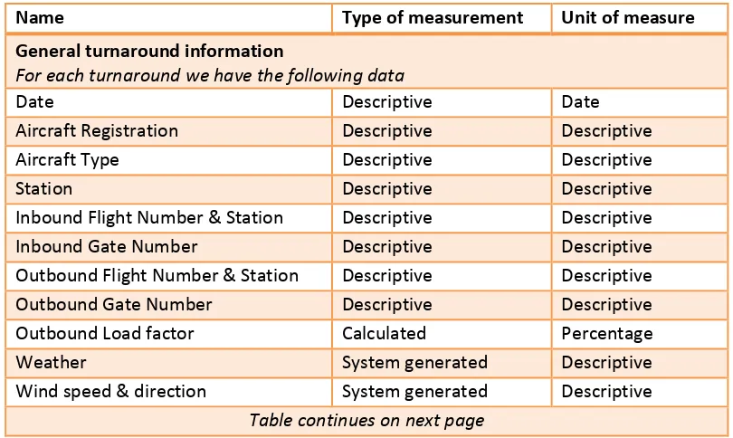
A general overview of all KPIs that are relevant for this research can be found in Table 5. In this overview we give the description, unit of measure, the frequency it is measured and indicate whether it is controlled using a target.
To manage the complex turnaround process and provide Service Level Agreements (SLAs) with its suppliers, KLC has established fifteen turnaround schedules that define which activities have to take place at what time during a turnaround. These fifteen different types are based on certain circumstances in which the turnaround has to be performed. These include the type of aircraft, which gate the passengers have to pass through, whether it is a quick turnaround (QTA) or not, and whether it is the first flight of the day. Each of these circumstances has a certain influence on the exact characteristics of the turnaround; an Embraer needs more time than a Fokker, because it is a larger aircraft and some activities thus take longer (cleaning, boarding of passengers). In a QTA, there is less time available for certain activities. Embraer flights leaving at the D-gate might use three busses instead of two, and finally, the first flight of the day only needs departure-oriented activities. The fifteen different turnarounds with their respective parameters can be found in Table 4, they are internally documented as ‘OCP-ZY20’. An example of one of these can be found in Appendix B.
Number Aircraft type
QTA Gate type First of
day?
1 F70 No Semi contact Yes
2 F70 No Platform Yes
3 F70 No Semi contact No
4 F70 No Platform No
5 F70 Yes Semi contact No
6 F70 Yes Platform No
7 E190 No Semi contact Yes
8 E190 No Platform Yes
9 E190 No Platform, D-gate Yes
10 E190 No Semi contact No
11 E190 No Platform No
12 E190 No Platform, D-gate No
13 E190 Yes Semi contact No
14 E190 Yes Platform No
General
Metric
Frequency
Target Description
D0
Percentage
D, W, M, Q, Y
Yes
% of flights in that period that leave on or before scheduled time
D15
Percentage
D, W, M, Q, Y
Yes
% of flights in that period that leave within 15 minutes of scheduled time
A0
Percentage
D, W, M, Q, Y
Yes
% of flights in that period that arrive on or before scheduled time
A15
Percentage
D, W, M, Q, Y
Yes
% of flights in that period that arrive within 15 minutes of scheduled time
Completion factor
Percentage
D, W, M, Q, Y
Yes
% of scheduled flights which actually have been flown
Registration changes
Number
D, W, M, Q, Y
No
Number of changes to which aircraft is assigned to a flight within 60 minutes of
departure
Non-performance departments
Hours
D, W, M, Q, Y
No
Sum of delay caused by each department of KLC, identified using delay codes
Non-performance within
department
Hours
D, W, M, Q, Y
No
Sum of delay caused by each activity within a given department, identified
using delay codes
Ground Services
Service providers ready at their
deadline
Boolean
M
Yes
Whether the given service was finished at its designated moment
Additional specific measurements with different service providers,
Example measurement with KE (fuelling service provider):
# Delays caused by fuelling
Number
M, Y
Yes
Count of delay codes assigned to fuelling
# Refuels
Number
M, Y
No
Count of total refuels in period
% Refuelling’s started before D-45
Percentage
M, Y
No
Percentage of refuelling’s started before D-45
# Defuels
Number
M, Y
Yes
Count of total defuels (e.g. due to cancelled flight)
# Additional fuel
Number
M, Y
Yes
Count of additional refuelling’s (e.g. due to changed weather conditions)
# Additional fuel after D-20
Number
M, Y
Yes
Count of additional fuel starts after D-20
% Refuels with >100KG overshoot
Percentage
M, Y
No
Percentage of refuels where the amount of loaded fuel was over 100 KG more
than requested
Flight Operations
Flight Plan / Fuel
Hours
M, Y
No
Sum of delay caused around flight- & fuel plan approval, code 57, 61 & 62
(Flight plan N/A, Flight plan change, addition fuel required)
Co Crew
Hours
M, Y
No
Sum of delay caused by Cockpit crew, code 63,64,65, 69 (late crew boarding,
crew missing, crew special request, captain requested security check)
The Gate type mentioned in Table 4 describes where the aircraft is located and where the scanning of the boarding passes of the passengers takes place. The aircraft can either be parked at the B-pier or on the platform, passengers can either be scanned at the B-pier or the D6-gate. A ‘semi contact’ departure means that the aircraft is parked at the B-pier and passengers are scanned at this pier as well. This allows passengers to, after their boarding passes are scanned, walk directly to the aircraft via two stairs without having to be transported by bus. A platform departure means that the aircraft is not parked directly at the gate and that passengers have to be transported to the aircraft first. For these departures, passengers can be scanned at either the B-pier and the D6-gate. After scanning, they are transported to the aircraft by bus. While most flights depart from the B-pier, this is not possible for all flights as some KLC destinations are not within the Schengen area, which means that movement of people and goods is not unrestricted. Examples of such destinations include the UK, Switserland, and Croatia. For these flights, an additional security clearance is needed, which Schiphol does not facilitate at the B-pier. Therefore, these flights have to depart from a special bus gate in the D-pier (D6-gate), where these facilities are offered. A section of the map of Schiphol where we marked the B-pier, D6-gate and platform can be found in Figure 4. Because of the larger distance, flights departing from the D6-gate with over 70 passengers are transported from the gate to the aircraft using three busses, all other flights ( all B-pier departures and departures with less than 70 passengers from the D6 gate) use a standard of two busses. Other gates on Schiphol, such as those on the C-pier or the F-pier, are not used by KLC.
A regular turnaround has a minimum ground time of 40 minutes for the Fokker F70 and 50 minutes for the Embraer E190. This distinction is made on the size of the aircraft. An Embraer can seat up to 100 passengers, compared to 80 for the Fokker. While a standard turnaround is often called a 40 minutes or 50 minutes turnaround, actual planned ground time can be far greater than that, as the mentioned 40 and 50 minutes are simply a minimum.
This chapter answers the second research question: What data is further required to assess the actual performance of the turnaround process? To answer this question, we first look (Section 3.1) at the current delay identification process, how it is performed, and what its caveats are. In Section 3.2, we then turn our attention to currently known or suspected influences on the D0 performance by interviewing KLC employees. We try to identify which activities are currently underperforming or which circumstances negatively influence D0 according to KLC employees, and supplement this with findings from literature. In Section 3.3, we look at the data available for this research. As part of the AP2K project, a central data gathering system is being built which gathers info from all parties involved in the turnaround process. The data in this system is made fully available for this research. We discuss the range of data and what it represents. In Section 3.4, we filter our dataset to exclude unnecessary, incomplete, and inconsistent data, to make sure that our findings in Chapters 4 and 5 are relevant and reliable.
As mentioned in Chapter 1, the current delay identification method is not waterproof. The codes are being assigned by hand by the Turnaround Coordinator (TLO) on duty; assignment is thus subject to the perception, opinion and knowledge of that specific TLO, resulting in not always properly assigned codes. For example, when the TLO notices that the boarding of passengers finished too late, he may assign code 15 (Boarding, Discrepancies, & Paging) as cause. However, the delayed boarding can also be caused by a preceding activity or other cause, e.g. code 67 (Cabin crew shortage), code 19 (Passenger with reduced mobility), code 17 (Catering Order Late/Incorrect) and many more. This requires a good overview of the entire process by the TLO and good communications between him and everybody involved in the turnaround process. However, given the often-hectic atmosphere during a delayed turnaround, this information may get lost, resulting in an incorrect delay code assignment. Another risk is that, given the large number of codes, the TLO simply does not know the right delay code to assign. Some codes are assigned more than others, resulting in the less used codes to be less known and maybe assigned even less. The final influence on the quality of the assigned delay codes is the number of delay codes that can be assigned. Currently only two codes can be assigned to a single flight, meaning that when there are more than two causes, this information gets lost. This means that while identifying causes of delay by using assigned codes is a good idea but in its current form its reliability depends on the skill, perception and honesty of the assigning TLO. This implies that although it is a good way to get a general impression of causes of delay, it is insufficient to gain true and decisive insights.
In this section, we try to identify which circumstances and activities are currently known or suspected to have a significant impact on D0 performance. These circumstances will be used as input variables in Chapter 4, where we test whether this information is correct. The primary source for these influences is internal knowledge at KLC supplemented with insights gained from literature. Special attention is given to the relation of departure punctuality to arrival punctuality of the preceding flight.
delayed and there is not sufficient ground buffer time, all activities and the departing flight will also be late. However, this delayed flight could not start any sooner, so is not accountable for its own delay. Therefore, we introduce a two-type classification of delay: propagated delay and contributed delay.
In this delay classification, propagated delay of a flight (say flight X) is delay caused by a preceding flight (flight Y) which could not be made up for by flight X (AhmadBeygi, Cohn, Guan, & Belobaba, 2008). A simple example: flight Y arrived 50 minutes late and, because there was no slack in the schedule, flight X also departs 50 minutes late. However, flight X manages to make up for some of the delay and arrives only 30 minutes past its original deadline. It would be unfair to hold flight X accountable for these 30 minutes delay as it even made up for some of the delay it received from flight Y. Therefore, we attribute the 30 minutes delay of flight X to flight Y. This delay propagation works on multiple levels; say we add a flight Z to the network, scheduled as predecessor of flight Y. flight Z started in time but finished 40 minutes late. In this case, the 50 minutes delay of flight Y were partly caused by flight Z being 40 minutes late, thus it would again be unfair to hold flight Y accountable for the full 50 minutes so we attribute 40 minutes to flight Z while keeping flight Y accountable for 10 minutes. Next to that, only 10 of the 30 minutes of delay of flight X are caused by flight Y. Therefore, the other 20 of these 30 minutes are in turn attributed to flight Z.
Flight Z Flight Y Flight X
Planned start 0 100 200
Actual start 0 140 250
Planned finish 100 200 300
Actual finish 140 250 330
Delta throughput time
+40 +10 -20
Propagated delay 0 60 30
Contributed delay 100 20 0
The HubDB is a database with vast amounts of data generated by KLM Ground Services, supplemented with various sources relevant for the ground process. Most of the sources mentioned hereafter are captured within the HubDB. However, because we believe information regarding the origin of data is useful we introduce the most important indirect sources individually.
AAS (Amsterdam Airport Schiphol), is responsible for the busses transporting passengers from the gate to the aircraft when it is a so-called platform departure. The drivers of these busses generate various data points, such as the time they are on position and waiting for passengers, the time the offloading of the passengers starts at the aircraft and the time offloading is completed. In this research, this data is used as an indicator for the performance of the passenger boarding process, as there is currently no other data available besides the scanning of the boarding passes at the gate. Unfortunately, the timestamps are generated manually by the driver of the bus and there might be a discrepancy between the actual event and the logged timestamp.
ACARS (Aircraft Communications and Reporting System), is a communication system linking aircraft to ground control. One of its uses, and the most relevant one for this research, is the logging of all system events generated by the aircraft before, during, and after a flight. Data gathered includes ‘first cargo door open’, ‘last cargo door closed’, ‘passenger door open’, and ‘passenger door closed’. Because this data is generated by the aircraft itself, it is highly reliable. Data from ACARS is gathered from the HubDB.
Axxicom is the company responsible for transporting unaccompanied minors (UM’s) and passengers with reduced mobility (PRM) from and to the aircraft. Information gathered from this source includes collection and drop-off time of the passengers. The timestamps we received from Axxicom are unfortunately also generated by hand.
CHIP, (Dutch: Communicatie & Hub Indelings-Programma) or Communication and Hub Scheduling programme, is the system KLM Ground Services uses for online operations scheduling of most tasks; TLO, cleaning, fuelling, cargo, toilet, water, and pushback. It has a constant feed of data of which tasks have to be performed at what gate and creates a load balanced schedule based on both priority and urgency of each task. Of each activity the planned start and end moment are registered, together with the actual start and end moments. Important to note is that the planned data is system generated while the moments at which the task was actually performed is generated manually by the operator. All CHIP data is gathered from the HubDB.
FIRDA, (Flight Information Royal Dutch Airlines), is the system in which flight data is recorded for every flight executed by KLM. Examples of data points include scheduled time of arrival (STA), actual time of arrival (ATA), and Estimate Block Departure (EBDE, adjusted scheduled departure time to accommodate circumstances such as a late incoming aircraft). Data from FIRDA is system generated and gathered from the HubDB.
The available data for this research was far from complete or unambiguous. Because not all service providers were able or willing to share their information, it proved to be hard to gather a full and complete set of data points. Effort was made to gather data ranging from 01-01-2014 until 01-06-2015. However, we did not succeed for all data providers. In Figure 6, an overview of all data sources and their availability are presented. As we see, most data is available for the entire timespan. However, Axxicom, AAS, and LVNL data is partially missing from our dataset. Unfortunately, we were unable to gather additional data from these sources.
When using empirical data for an analysis, one must make sure that the observed data is reliable and validated (Flynn, Sakakibara, & Schroeder, 1990). In our analysis, this means that we need to exclude any obviously incorrect or irrelevant data to improve reliability of the results. For this purpose, we set up a set of exclusion rules that we applied to the data. These rules were verified and justified by KLC to make sure we did not exclude relevant data. These rules are:
Not all of our data concerns regular turnarounds. Sometimes an aircraft cannot fly due to technical failures or damages and a replacement aircraft has to be used to perform the flight. If this happens at an outstation, often no replacement aircraft is present and it has to be flown in from AMS. This ‘aircraft placement flight’ has no passengers on board and is logged with a special flight number to differentiate it from regular flights. Because no full servicing is needed and departure delay is not of influence to total KLC numbers, these flights should not be taken into consideration.
A delay of over 3 hours is unlikely to be caused by regular delay causes. Often it is a disruptive cause that cannot be anticipated or circumvented, e.g. the closing of the airport due to a terrorist threat or a technical malfunction. Because we have no information regarding the occurrence of these exceptional causes and their predictability is low, we eliminate these turnarounds from our data.
An aircraft can only depart when all passengers are present and boarded, which is unlikely to be the case more than an hour before scheduled departure. Therefore, a departure of more than 60 minutes early indicates special circumstances or a data error. Both are unwanted in our dataset.
The planned turnaround time is the time difference between the scheduled time of arrival (STA) and scheduled time of departure (STD). When this time is negative, i.e. the aircraft is scheduled to depart before it is scheduled to arrive, this indicates a data error and we eliminate it from our dataset. Similar, when either STA or STD is missing, planned turnaround time cannot be determined and the turnaround is eliminated from the dataset.
To get a thorough and reliable understanding of delay causes, it is necessary to have consistent measurements. When parts of the data of a single turnaround are missing, no reliable conclusion can be drawn as delay might be caused by a missing variable. Therefore, we have limited our dataset to include only turnarounds for which the measurements of all major activities are present. These activities include baggage, fuel, toilet, catering, cleaning, crew transport, and boarding pass scans. Some activities are left out of this list because they do not necessarily occur every turnaround. Busses are only needed when departing from the platform, Axxicom is only needed when there is a PRM or UM present, pushback is not always needed as some parking spots can be exited in a forward movement and water is sometimes multi stretched, meaning multiple flights are performed on a single load.
To exclude obvious data errors, we eliminated all turnarounds for which any activity had a timestamp outside logically possible boundaries. For example, when the operator of the toilet cleaning truck ‘completes’ his task after the aircraft departed, it is an obvious error. We decided not to place these boundaries exactly at actual arrival and departure, because sometimes servicers start their activity when they start to drive towards the location of the aircraft, thus ‘starting’ before the aircraft actually has arrived. For example, the Baggage handling operators start their activity when they start loading baggage onto their trucks at the baggage collection point. At departure, we have the same situation. A clear example is the pushback operator. He finishes his task when the aircraft is pushed back, thus after the actual departure (which is equal to the moment he starts pushing). We set our boundaries differently for each of the major activities to make sure they are not too loose for some activities, or too restrictive for others.
Activity Turnarounds Total Faulty*
Missing Out of Bounds
Short Duration
Extreme Duration
Bax ** 69,901 1,954 642 1,081 105 214
Cleaning ** 69,901 1,792 462 346 170 937
Crew Transport 69,901 17,260 1,408 960 1,931 13,632
Fuel ** 69,901 2,234 407 956 114 874
Extra Fuel 69,901 67,626 67,574 41 15 -
Toilet ** 69,901 2,240 597 521 852 429
Water 69,901 18,099 17,444 143 - 536
Catering ** 69,901 11,468 7,187 15 1,459 2,811
PaxScan ** 69,901 3,788 304 2,658 811 2,336
TLO 69,901 45,935 197 12,464 286 42,936
Pushback 69,901 26,827 24,069 154 2,580 80
Arrival Bus 69,901 53,202 51,635 276 1,308 2
Departure Bus 69,901 52,214 52,149 56 6 3
Arrival Axxicom 69,901 62,419 60,879 663 1,197 11
Departure Axxicom 69,901 65,214 64,141 21 6 1,060
Event
CDO 69,901 31,167 31,127 40 N/A N/A
CDC 69,901 28,101 28,089 12 N/A N/A
PDO 69,901 28,294 28,251 43 N/A N/A
PDC 69,901 28,015 28,005 10 N/A N/A
* Number of turnarounds with at least one faulty or missing measurement ** Activities that need to be present and not faulty
Rule Nr of dropped turnarounds
Turnarounds left in dataset
Start - 70,099
Outbound flight should be a regular flight with passengers
103 69,996
Outbound flight should be to a regular destination 15 69,981 Total planned turnaround time should be non-negative 33 69,948 Outbound flight should be no more than 3 hours
delayed
46 69,902
Outbound flight should not depart more than 60 minutes early
1 69,901
All measurements of all major activities should be present, within bounds and a have logical duration
22,781 47,120
In this chapter, we discuss the results from the analysis into departure delay. We first discuss the general performance regarding duration, start and finish times of the activities during a turnaround (Section 4.1), after which we introduce decision tree learning and perform this on our data to find relations between circumstances or activity characteristics and departure delay (Section 4.2). In Section 4.3, we compare our delay classification to the current delay coding system to see which of these two gives a more reliable indication of the cause of delay.
In this section, we discuss the performance of the various activities during a turnaround by looking at duration (Section 4.1.1), completion time (Section 4.1.2), and starting time (Section 4.1.3). Note that for the completion time and starting time, we use the variables ‘Dminus’ and ‘Aplus’ that we determined from our data. The Dminus variable is the time between the completion of the task and a modified departure time. This departure time is the latest of any of three variables: Scheduled time of departure (STD), Estimated Block time (EBDE) and the minimum ground time. The latter was added to ensure service providers receive enough time to perform their activities, even when KLC did not set an EBDE to account for arrival delay. The Aplus variable is the time between the activity start moment and actual arrival, a performance measurement useful for
arrival-oriented activities. Figure 7 visualises these two variables, along with a few others. Note that arrival oriented and departure oriented targets and performance is expressed as ‘A+#’ or ‘D-#’, where ‘#’ can be any number, e.g. A+3 or D-3. This indicates that the target for that activity is set as ‘3 minutes after arrival’ or ‘3 minutes before departure’. Consequently, when reading the tables in Section 4.1, note that an activity with a target of A+3 and a performance of 4 (or A+4) is under performing, as it is after target. At the same time, an activity with a target of D-3 and a performance of 4 (or D-4) is over performing, as it is before target. Note that due to confidentiality the numbers in this section are altered and cannot be used as a reference for actual performance.
Looking at Table 11, most activities seem to perform very well with an average duration that is similar to or smaller than its target. One activity stands out negatively: crew transport has an average duration of 21.61 minutes versus a target of 12 minutes. The explanation for this lies in the fact that the department responsible for crew transport does not use its planned CHIP times for anything other than to assign a job to a driver and thus not as a target. Because the actual duration can vary greatly depending on where the crew has to be picked up and delivered, the standard deviation of 14.90 minutes is also high. Note that we excluded durations of over 60 minutes in this overview. This is to prevent first of day turnarounds with multiple activities to skew the results. We discuss this in more detail in Section 4.1.3.
In order to measure the performance of the various activities with regard to their completion time, we have to perform two steps. First, we have to make sure we measure the right performance and in order to do this, we determine the moment we want to compare the activity completion time with. Comparing it to the Actual time of departure (ATD) is not a good idea because when a flight is delayed, activities that caused the delay will seem to perform normal, while activities in that same turnaround that finished in time will seem to perform better than expected. Therefore, we set the baseline to be either of three moments in time: scheduled time of departure (STD), minimum ground time departure (minSTD) or Estimate Block Departure (EBDE). The STD is the originally scheduled time the aircraft should depart and is always present in our data. The minSTD is the time at which the minimum turnaround time (35 minutes, 40 minutes or 50 minutes) is passed after arrival. This is useful when the incoming flight is delayed, as operators still need their minimum time to complete their task. The EBDE is an adjusted scheduled departure time when an aircraft cannot depart sooner due to external reasons. This might for example be due to a severely delayed incoming flight, technical difficulties or restrictions at the airport. Of these three times, we take the one that represents the latest moment in time and determine the difference in minutes between that time and the activity completion time. This number of minutes before departure is stored in the variable D-minus and compared to the target completion time in Table 12.
The other type of machine learning is unsupervised learning. Here, we do not have a ‘supervising’ variable to which we relate the other variables, but rather every variable is equal. Thus, unsupervised learning tries to cluster its input variables together in any way possible, not just to a single response variable. Again looking at Table 14, unsupervised learning will look for any combination of these variables. For example, it might identify that if people smoke, they also tend to be a drinker. (Van der Aalst, 2011)
Smoker Drinker Weight Age of death
Yes Yes 110 Young
No No 60 Old
Yes Yes 100 Young
No No 95 Old
No No 70 Old
… … … …
No Yes 120 Young
Yes No 80 Old
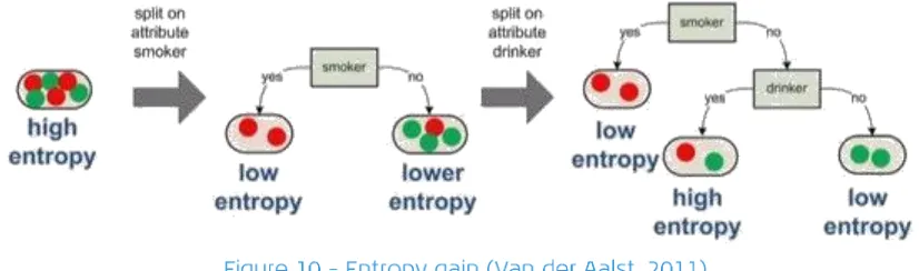
For our goal, we clearly need a supervised learning technique, as we want to classify variables on whether they cause delay or not. The most used supervised learning technique is Decision tree learning. This technique builds a tree of predictor variables, with every branch being a certain value of a variable. A simple example is given in Figure 9, where we present a tree based on the entire dataset of Table 14. In this tree, we try to predict the age at which people die, based on the various variables present in the dataset. The way decision tree learning works is that it takes the entire dataset and tries to divide this dataset on every available variable. In our example, it will try to divide our data on the smoking variable, the drinking variable and the weight variable. Its goal is to gain a better classification of the response variable, where its ideal output would be a perfect classification, where in every end node all entries have the response variable value in which it was classified. Before we discuss the way the tree is ‘learned’, we give a small explanation on how to read a decision tree: We start with the root node, where we split the data into two branches, based on the first chosen variable, in this case ‘smoking’. Each branch is classified, or predicted, to die at either an old or a young age. In this case, if the subject was a smoker, the person is
In order to identify relations between circumstances and departure delay, we use two methods. First, we apply decision tree learning to look for predictor variables in our dataset that correspond to departure delay. For this purpose, we choose our experimental design in Section 4.3.1, where we determine the input parameters for our algorithm. Next, in Section 4.3.2, we present and discuss the results. We have visualised the steps of the decision tree learning process in Figure 11. In addition, we use the delay propagation method we introduced (Section 3.2.1) to look for activities within a turnaround that were delayed and, according to the propagation algorithm, delayed the entire turnaround.
Before presenting the results, we first discuss how we instruct our decision tree learning process which data to use and what settings it should take into account. In other words, how we make sure that the results from our analysis are relevant and not influenced by selecting bad parameter settings. In order to select the correct parameters values, we used multiple runs, each with a different combination of parameter values.
Because of the large number of parameter values that we have to choose, we divide them into three categories, namely input data related, random forest related and decision tree learning related. When testing the different parameter values, we perform an incremental design. First, we test the various combinations for the input data related parameters. From these, we select the best predicting combination and continue to test the performance of the second set, the random forest related parameters. Again, this results in a set of best performing parameter values, which we then use to determine the best combination of parameter values in the decision tree learning related category. This will result in a good combination of parameter values that we can feed to our algorithm.
In Chapter 3, we presented the dataset we use as input for our decision tree learning process. However, within this dataset, we have a few options regarding what data we actually use, as we have various variables that describe similar performances. For example, for each activity, we have the time between scheduled departure and activity completion time, but also the deviation of activity completion time to its target completion time (Table 7). As these variables represent similar performance, we need only use one of these types of data. Next to that, we also want to test whether using the dummy data generated for the random forest (Table 17) would also improve performance for our decision tree learning process.
Number of trees: 5000 Table continues on next page
Minimum resulting leaf from branch 30
Number of variables per tree 10
Decision tree learning related:
Minimum size of leaf before trying to branch 60
Minimum resulting leaf from branch 30
Minimum information gain from branch 0.005
Maximum depth of tree 30
The final general variable is load factor. Regardless of aircraft type, when load factor is above 91%, the flight is predicted to be delayed. A logical explanation is that the duration of some activities depends on the number of passengers present. For example, the number of bags to be placed into the cargo hold increases, the time needed to scan all boarding passes increases, the time needed to get everybody seated within the aircraft and cabin luggage stowed away increases, and so on. Target processing times were determined based on activity durations under full load, but without disturbances. Thus, a single disturbance can disrupt the process, lengthen activity duration and delay the flight, because there is no slack time to make up for it. When the load factor is low, activities have more slack, allowing for some disturbances.
Finally, a variable that was only present in Embraer turnarounds: the RTD lateness. This is the time between the closing of the last door and the captain notifying the tower that he is ready to depart. RTD lateness might be caused when passengers have not taken their seat yet, or cabin luggage that has not been stowed away properly. Especially for flights with a high load factor this is an issue, as the amount of luggage people carry will be close to the maximum capacity of the luggage holds, and people will have to search for a place to stow their luggage. Nevertheless, although we could not determine the RTD lateness for the other turnarounds, because we do not have door closure data from the Fokker, we expect the RTD lateness to have an influence on Fokker turnarounds as well, because luggage and seating issues also occur in the Fokker.
delay is already calculated for the entire data set for the AP2K project, we can easily compare the results from the entire set with the results of the filtered data set. This comparison is presented in Table 24. Although small differences occur, no major differences exist between the two sets. Of course, this is just a very rough comparison and further research is required before any hard conclusions can be drawn, but it seems that the filtered data is a good representation of the entire data set.
In this section, we discuss the quality of the current delay identification method by comparing the delay attributed to a specific code to our data. Because it is the most frequently assigned delay code, (over 18% of all flights receive a code 89) and we have good comparison values in our data, we perform this comparison primarily on code 89, which stands for ‘Restrictions at departure airport’, or the most common cause: no departure slot made available by local air traffic control (Local ATC). This code should be assigned when the aircraft is fully ready to depart and departure is requested at local ATC (RTD notification), but local ATC does not have a free departure slot available, ordering the aircraft to wait at the gate before it can be pushed back. Because a TLO cannot see whether an aircraft is not departing due to an unready cabin or because of Local ATC restrictions, KLC suspects code 89 to be given too often.
Using our data, we can determine the actual delay caused by Local ATC by calculating the time between the Ready to depart notification and actual departure, which we call Local ATC lateness. When the delay code has been assigned correctly, this amount of minutes should be equal to the amount of delay minutes assigned to code 89, either as primary delay code or as secondary delay code. In Figure 14, we plotted the comparison between these two, where we allowed a minute of
deviation between the two times due to rounding errors or human error.
determined, and ‘assigned code 89 minutes’ indicates the amount of ATC delay that was assigned by the TLO.
However, in Figure 14, we also see that in roughly 30% of the cases our data suggests that the amount of assigned Local ATC delay is actually too low when compared to the time between the ready to depart notification and actual departure. Looking deeper in our data, we notice that for over 400 flights the RTD lateness (time between all doors closed and RTD notification) was negative, indicating that the RTD notification was given before the doors were closed, which would be impossible by its definition. KLC Flight Operations confirmed that this indeed is a possibility, as sometimes pilots give a RTD notification prematurely when they expect a long Local ATC delay. For example, the pilots expect they will be ready for take-off in 5 minutes but they notice on the radio that the current average waiting time for a departure slot is 10 minutes. In such a situation, they might give the RTD notification prematurely, to prevent having to wait the full 10 minutes after they are ready. Although the local ATC is indeed causing delay in such cases, it cannot be held responsible for causing 10 minutes of delay (the time between RTD and actual departure) which we currently do in our comparison, but only for the time after the aircraft is actually ready. In some cases, pilots may expect a delay in slot assignment, where in reality there proves to be none. In this case, the pilots give the RTD notification 5 minutes early, after which they are granted a departure slot immediately. At this moment in time, the aircraft still has to be prepared, still leaving 5 minutes after the RTD notification. In our comparison, these 5 minutes would wrongfully be attributed to Local ATC. A graphical explanation of this is represented in the left figure of Figure 16.
However, despite these limitations, we can still draw some conclusions on these findings. First, the statement that 11% of all flights receive too much code 89 delay still holds. While pilots can request a RTD notification too early, they cannot do this retroactively. This means that in our calculation, we can attribute too many minutes to local ATC, but not too few, meaning that the value we determined can be seen as the maximum amount of delay that could be caused by local ATC. When the assigned code 89 minutes exceed this, too much delay was attributed to local ATC. At the same time, less than 1% of all flights in our dataset have a negative RTD lateness, this number would be much higher if pilots send out a RTD notification prematurely for nearly 30% of all flights. We thus expect the percentage of incorrect assignments within this 30% of all flights to
be significant, however, this is something we cannot quantify.
Looking at code 89 only, it is safe to say that the current delay identification method is far from perfect. For at least 10% (and presumably significantly more) of all flights, the amount of delay attributed to local ATC (code 89) is incorrect. Of course, as stated in Chapter 1, delay identification is a difficult process, as the TLO should have constant focus on every step in the turnaround to ensure proper root cause analysis, and even then, he or she still might miss vital information. Also, code 89 is the most commonly assigned code, which makes it susceptible for being a ‘scapegoat’ for when the TLO does not know the exact cause. Finally, currently only two codes, or causes, can be given to a delayed flight. When three or more disturbances occur, this information gets lost. All this uncertainty surrounding delay codes makes it impossible for them to be used as a reliable input in a process performance analysis.
Based on the data analysis in this chapter, a few interesting conclusions can be made. First, important to note is that, while being very different techniques, the decision tree learning algorithm and delay propagation method show similar results. This means that it is safe to assume that these results show (at least for a large part) the true reasons behind departure delay.
When we start analysing the results from our decision tree learning algorithm in Table 23, we see that most of the delay originates at activities performed in the final stages of a turnaround. Scanning the boarding passes, closing the cargo doors, waiting for departure clearance from local ATC, all these activities are performed at the end of the turnaround. This makes sense, as, especially during a turnaround with a standard duration, there is some slack available between tasks. Thus, tasks at the beginning of the turnaround can be delayed without directly influencing departure punctuality. At the same time, the aircraft is scheduled to be ready for departure at D0, at which moment in time it can request departure clearance from local ATC. This means that for this event, no slack time is available and, unless previous tasks completed early, any delay in getting departure clearance will result in a delayed departure.
When an activity has multiple dependencies, we take the dependency that was finished last and use this as input for our slack calculations. Three examples on how we determine slack can be found in Figure 17. The first example is a regular calculation; a task has multiple dependencies of which we take the time the last one was finished to determine the activity slack. The second example shows how we handle activities that do not have dependencies; we take the planned starting moment from the OCP-ZY20 document. The third example shows an exceptional situation, namely that activities start before their dependencies, resulting in negative slack. As discussed in Section 4.3, this might happen with the ready to depart notification. The pilots request a departure slot prematurely, which results in a ‘negative’ slack. As this negative slack represents actual behaviour, we decide to leave this data in our input data.
Each turnaround is simulated in a single replication; we do not simulate turnarounds on a schedule level over the day. This is done because we only have detailed information of turnarounds at Schiphol. All outstation turnarounds and flights would simply be an historical duration, which adds little value to our model, and might even result in less realistic results, as we do not know whether changing departure punctuality may influence flight duration for example. Therefore, we see each turnaround as a single process, starting the simulation at aircraft arrival, and ending it at departure. However, there is a limited number of operators available for each task and by recreating each simulation independently, we would lose capacity constraints between simultaneous turnarounds we could model when recreating an entire day of fleet movements. For this purpose, we only use historical data from turnarounds that took place in a similar departure bank and comparable planned ground time. This way, historical non performance caused by resource constraints is still maintained within the model.
For our simulation, we use a terminating model, with empirical data as input. As we simulate each turnaround separately, the starting state and ending state of each run are unimportant. The aircraft arrives at a certain moment in time, and departs again after all tasks have been processed. After departure, the model is empty and the simulation stops. Therefore, we do not need any warming up period.
Using a 12-core CPU and creating 2200 replications per scenario, the entire model takes 12 hours and 43 minutes to complete. The results can be found in Table 29 where we listed the average departure punctuality (D0) per scenario per turnaround type. Notice that for the second scenario, the results of the standard turnarounds are missing. This is because this scenario only affects the QTA turnarounds, thus no simulation of the turnarounds with regular ground time was needed. First, we compare our ‘original’ scenario with the historical data. In the original data, we did not alter any parameters within the model; it thus should give similar performance as the historical data. We note that for some turnaround types, the historical data is more closely approximated than with the others, but the differences in D0 distribution are consistent. In Figure 18, we see a comparison of the D0 distributions between the simulations and the historical data. The observed D0 is placed on the horizontal axis, the vertical axis represents the number of observations. Also, the blue line represents the historical observations, whereas the orange line represents the simulated observations. The simulated results are slightly skewed to the right, which results in a higher average departure delay. Therefore, note that the delay of the original scenario does not represent actual delay. However, as the distributions are similar, the results of the different scenarios are representable, meaning we can expect similar effects on departure punctuality in real life as we get from our simulation model.
slack to be found in the process. At the same time, improving the A0 with 5 minutes seems to have a slight positive influence on D0 of the quick turnarounds, but this effect is very small.
KLC currently uses 15 turnaround types to define its turnaround processes. KLC management asked us whether they could reduce this number, without deteriorating departure delay. This means combining the various turnaround type schedules into a single schedule. Due to the fundamental differences between a standard turnaround and a quick turnaround, we decided to create a different turnaround type for each of these two, effectively reducing the number of turnaround types in our simulation model from six to two. The two different scenarios we test are described in Section 5.3.2. First, the second scenario we test shows a slight improvement for the semi contact departures, no improvement at the platform turnarounds and a deterioration of departure punctuality for the D6-gate departures. This is probably caused by the scheduled start of the boarding pass scans and the busses, in the second scenario, this is set to D-24. This is the same time as the current platform ZY20s, 7 minutes earlier than in the current semi contact ZY20s and 3 minutes later for the D6-gate ZY20s. This seems to directly influence the departure punctuality.
In the first scenario, we picked all the earliest possible times from every turnaround type, resulting in a significant improvement at both the platform and semi contact departures, but no improvement at the D6-gate departures. Again, this can mostly be explained by looking at the start of the boarding pass scanning process. In this scenario, we start a full 10 minutes earlier during semi contact turnarounds, and 3 minutes earlier during platform turnarounds. The D6 gate showed little to no improvement, as the created turnaround schedule is nearly identical to the current D6-gate schedule.
In this final chapter, we summarize the results from the previous chapters to find an answer to our main research question. To this end, we first do a short recap of our work and answer the sub research question in Section 6.1, after which we answer our main research question and discuss the implications for KLC in Section 6.2. In Section 6.3, we discuss the limitations of this research, and do some suggestions for further research.
This section is meant as a summary of the results of Chapters 2, 3, 4 and 5 and the answers to the research questions they provide. First, we look back at the current performance measures of Chapter 2 (Section 6.1.1), after which we discuss our data gathering process of Chapter 3 (Section 6.1.2). In Section 6.1.3, we discuss the data analysis of Chapter 4. Finally, in Section 6.1.4, we discuss our simulation and its results.
KLC uses many key performance indicators (KPIs) to get insight into its general performance. Each day, the overall results of the previous day are discussed, using delay codes to identify delay sources. These delay codes are also used to discuss performance during monthly performance meetings with the various service providers, comparing their actual performance (measured in number of assigned delay codes) to the agreed service levels in the service agreements. KLC uses procedures for 15 different combinations of turnaround circumstances, for each turnaround type defining at what time each activity or event should take place. These 15 turnaround types are based on aircraft type, planned ground time, aircraft location and gate location.
Thus, KLC has a thorough overview of how the turnaround process should happen, and has made agreements (both qualitative and quantitative) with its service providers towards this goal. KLC currently uses delay codes to identify causes of non-performance and gain insight into service provider performance. However, while this may give a general impression of performance, it is by no means an extensive tool to monitor the actual performance. Non-performance is only registered in a delay code when it has caused the aircraft to be delayed and, more importantly, when the TLO has identified the correct cause.
Finally, we present some topics that KLC should perform further research on, to gain more control over its departure punctuality. The first and most important topic is the number of busses used to transport passengers from the gate to the aircraft. Currently, KLC uses two busses from both the B-pier as well as the D6-gate, unless more than 70 passengers are expected at the D6-gate, in which case three busses are used. This third bus allows more spread in the arrival of the passengers at the aircraft, enabling a smoother boarding process. We performed a small initial data analysis into the departure punctuality for turnarounds departing from the D6-gate. We compared the performance of departures where two busses were used with departures where three busses were used. This showed that departures where three busses were used had an average D0 that was 1.5 minutes lower when compared with turnarounds with two busses. Further research into confirming this find is recommended and when successful, a pilot to use three busses at the B-pier might be worthwhile.
Next, in this research we use the ‘ready to depart’ notification to determine local ATC lateness. However, more data regarding the communication between the cockpit and the tower should be available. By examining this data, KLC might gain valuable insights into how it can reduce delay caused by waiting for departure clearance.
AhmadBeygi, S., Cohn, A., Guan, Y., & Belobaba, P. (2008). Analysis of the potential for delay propagation in passenger airline networks. Journal of Air Transport Management , 221-236.
Allison, P. (2009). Missing Data. In R. E. Millsap, SAGE Handbook of Quantitative Methods in Psychology (pp. 72-89). Thousand Oaks, CA, USA: Sage Publications Inc.
Cook, A., Tanner, G., & Lawes, A. (2012). The Hidden Cost of Airline Unpunctuality. Journal of Transport Economics and Policy , 157–173.
Flynn, B., Sakakibara, S., & Schroeder, R. (1990). Empirical research methods in operations management. Journal of Operations Management , 250-284.
Graham, J. (2009). Missing Data Analysis: Making It Work in the Real World. Annual Review of Psychology , 549-576.
Hsiao, C.-Y., & Hansen, M. (2006). An Econometric Analysis of US Airline Flight Delays with Time-of-Day Effects. Berkeley: National Center of Excellence in Aviation Operations Research.
Kohla, N., Larsen, A., Larsen, J., Ross, A., & Tiourine, S. (2007). Airline disruption management - Perspectives, experiences and outlook. Journal of Air Transport Management , 149–162.
Law, A. M. (2007). Simulation Modeling & Analysis. Tucson, Arizona, USA: McGraw-Hill.
Mladenic, D. (2005). Feature Selection for Dimensionality Reduction. Subspace, Latent Structure and Feature Selection (pp. 93-102). Bohinj, Slovenia: Springer.
Oshiro, T., Perez, P., & Baranauskas, J. (2012). How Many Trees in a Random Forest? International Conference on Machine Learning and Data Mining (pp. 154-168). Springer.
Reif, D., Motsinger, A., McKinney, B., Crowe Jr, J., & Moore, J. (2006). Feature Selection using a Random Forests. IEEE.
Tu, Y., & Ball, M. (2008). Estimating Flight Departure Delay Distributions - A Statistical Approach With Long-term Trend and Short-term Pattern. Journal of the American Statistical Association , 112-125.
van der Aalst, W. (2011). Process Mining. Heidelberg: Springer.
Winston, W. L. (2004). Operations Research. Belmont California, USA: Thomson Brooks/Cole. Witten, I., & Frank, E. (2000). Data Mining. San Diego: Morgan Kaufmann Publishers.
Wu, C., & Craves, R. (2004). Modelling and Simulation of Aircraft Turnaround Operations. Transportation Planning and Technology , pp. 25–46.
Wu, C.-L. (2008). Monitoring Aircraft Turnaround Operations - Framework Development, Application and Implications for Airline Operations. Transportation Planning and Technology , 215 - 228.
Wu, C.-L., & Caves, R. E. (2003b). The punctuality performance of aircraft rotations in. Transportation Planning and Technology , 417–436.
TLO Dutch: Team Leider Omdraai. Person managing the turnaround, present and responsible the entire on-blocks time.
Hub-and-Spoke network Plan of flights where all destinations are served from a single airport
Flight Operations Department of KLC responsible for all flight operations
KLC KLM Cityhopper
KLM Royal Dutch Airlines (Dutch: “Koninklijke Luchtvaart Maatschappij”)
Loadsheet List of all people and items on board of the aircraft.
Multi-stretching Skipping an activity between flights, e.g. no water replenishment
OCP-ZY20 KLC Procedure describing the turnaround process
Outstation Airport to which KLC maintains a flight connection from Amsterdam
Terminal weather The local weather at the airport
Platform Section of the airport where aircraft are parked during a turnaround if
not at a gate.
Registration change The assignment of a different aircraft to perform a certain flight.
STA / ATA Scheduled time of arrival / actual time of arrival
STD / ATD Scheduled time of departure / actual time of departure
PDO / PDC Passenger door open / passenger door closed
OCP-ZY20 - List of activities during a turnaround at AMS of an Embraer 190, taking 35 minutes and departing from the platform
The weekly report regarding ground process performance as created by the Manager Operational Processes & Planning to be used by the Director Ground Services & Cargo Operations KLC. (2 pages)
Removed due to confidentiality
Monthly non-performance overview Ground Services (ZY) on all stations, also created by the Manager Operational Processes & Planning to be used by the Director Ground Services & Cargo Operations KLC.
Removed due to confidentiality
Monthly non-performance comparison of Ground Services at Schiphol, non-performance compared to same month last year. Again created by the Manager Operational Processes & Planning to be used by the Director Ground Services & Cargo Operations KLC.
Removed due to confidentiality
The weekly report regarding ground process performance in Amsterdam, supplemented with specific service provider activity overviews, created by the various Duty Managers Ground Services. Below the specific performance chart for the water and toilet service for week 3 in 2015.
Monthly summary of task conformance during turnarounds, as monitored by the Duty Managers Ground Services. Summary is in shape of Excel file, with performance divided over tabs, each area of attention has a separate tab. Below are the general tab and loading-specific tab for April 2015.
Removed due to confidentiality
Tab with Loading-specific performance:
Performance overview KLC Flight Operations (ZV) used by (among others) Director Flight Operations.
Removed due to confidentiality
Weekly report regarding operational performance created by Operations Control (ZZ) to be used in weekly management team (MT) meeting of KLC.
Removed due to confidentiality
Performance conformance checklist used during turnarounds by the Duty Managers Ground Services. Used as input for the summary in appendix H.
Data availability of the different tasks
Activity Turnarounds Total
Faulty