Retrieval Term Prediction Using Deep Belief Networks
Qing Ma† Ibuki Tanigawa† Masaki Murata‡
†Department of Applied Mathematics and Informatics, Ryukoku University ‡Department of Information and Electronics, Tottori University
Abstract
This paper presents a method to predict re-trieval terms from relevant/surrounding words or descriptive texts in Japanese by using deep belief networks (DBN), one of two typical types of deep learning. To determine the effec-tiveness of using DBN for this task, we tested it along with baseline methods using example-based approaches and conventional machine learning methods, i.e., multi-layer perceptron (MLP) and support vector machines (SVM), for comparison. The data for training and test-ing were obtained from the Web in manual and automatic manners. Automatically cre-ated pseudo data was also used. A grid search was adopted for obtaining the optimal hyper-parameters of these machine learning meth-ods by performing cross-validation on training data. Experimental results showed that (1) us-ing DBN has far higher prediction precisions than using baseline methods and higher pre-diction precisions than using either MLP or SVM; (2) adding automatically gathered data and pseudo data to the manually gathered data as training data is an effective measure for fur-ther improving the prediction precisions; and (3) DBN is able to deal with noisier training data than MLP, i.e., the prediction precision of DBN can be improved by adding noisy train-ing data, but that of MLP cannot be.
1 Introduction
The current Web search engines have a very high retrieval performance as long as the proper retrieval terms are given. However, many people, particularly
children, seniors, and foreigners, have difficulty de-ciding on the proper retrieval terms for represent-ing the retrieval objects,1 especially with searches related to technical fields. The support systems are in place for search engine users that show suitable retrieval term candidates when some clues such as their descriptive texts or relevant/surrounding words are given by the users. For example, when the relevant/surrounding words “computer”, “previous state”, and “return” are given by users, “system re-store” is predicted by the systems as a retrieval term candidate.
Our objective is to develop various domain-specific information retrieval support systems that can predict suitable retrieval terms from rele-vant/surrounding words or descriptive texts in Japanese. To our knowledge, no such studies have been done so far in Japanese. As the first step, here, we confined the retrieval terms to the computer-related field and proposed a method to predict them using machine learning methods with deep belief networks (DBN), one of two typical types of deep learning.
In recent years, deep learning/neural network techniques have attracted a great deal of attention in various fields and have been successfully applied not only in speech recognition (Li et al., 2013) and image recognition (Krizhevsky et al., 2012) tasks but also in NLP tasks including morphology &
syn-1For example, according to a questionnaire
admin-istered by Microsoft in 2010, about 60% of users had difficulty deciding on the proper retrieval terms. (http://www.garbagenews.net/archives/1466626.html)
Labels (Retrieval terms)
Inputs (Descriptive texts or relevant/surrounding words; translated from Japanese)
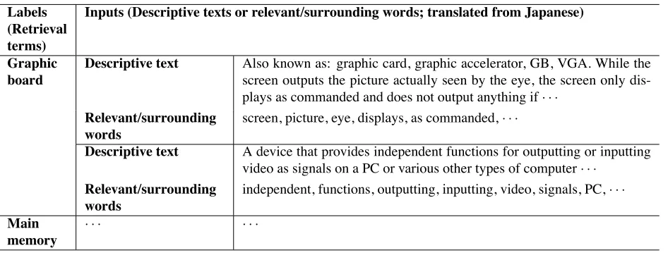
Graphic board
Descriptive text Also known as: graphic card, graphic accelerator, GB, VGA. While the screen outputs the picture actually seen by the eye, the screen only dis-plays as commanded and does not output anything if· · ·
Relevant/surrounding words
screen, picture, eye, displays, as commanded,· · ·
Descriptive text A device that provides independent functions for outputting or inputting video as signals on a PC or various other types of computer· · ·
Relevant/surrounding words
independent, functions, outputting, inputting, video, signals, PC,· · ·
Main memory
· · · ·
Table 1: Examples of input-label pairs in the corpus.
manually gathered data and (2) for each label, ran-domly adding the words that were extracted in step (1) but not included in the descriptive texts and/or deleting words that originally existed in the descrip-tive texts so that the newly generated data (i.e., the newly generated descriptive texts) have 10% noises and/or deficiencies added to the original data.
2.3 Testing Data
The data described in Subsections 2.1 and 2.2 are for training. The data used for testing are different to the training data and are also obtained from automat-ically gathered data. Since automatautomat-ically gathered data may include a lot of incorrect labels that cannot be used as objective assessment data, we manually select correct ones from the automatically gathered data.
2.4 Word Extraction and Feature Vector Construction
Relevant/surrounding words are extracted from de-scriptive texts by steps (1)–(4) below and the inputs are represented by feature vectors in machine learn-ing constructed by steps (1)–(6): (1) perform mor-phological analysis on the manually gathered data and extract all nouns, including proper nouns, ver-bal nouns (nouns forming verbs by adding word
(suru, “do”)), and general nouns; (2) connect the nouns successively appearing as single words; (3) extract the words whose appearance frequency in each label is ranked in the top 50; (4) exclude the words appearing in the descriptive texts of more
than two labels; (5) use the words obtained by the above steps as the vector elements with binary val-ues, taking value 1 if a word appears and 0 if not; and (6) perform morphological analysis on all data described in Subsections 2.1, 2.2, and 2.3 and con-struct the feature vectors in accordance with step (5).
3 Deep Learning
Two typical approaches have been proposed for im-plementing deep learning: using deep belief net-works (DBN) (Hinton et al., 2006; Lee et al., 2009; Bengio et al., 2007; Bengio, 2009; Bengio et al., 2013) and using stacked denoising autoencoder (SdA) (Bengio et al., 2007; Bengio, 2009; Bengio et al., 2013; Vincent et al., 2008; Vincent et al., 2010). In this work we use DBN, which has an elegant ar-chitecture and a performance more than or equal to that of SdA in many tasks.
DBN is a multiple layer neural network equipped with an unsupervised learning based on restricted Boltzmann machines (RBM) for pre-training to ex-tract features and a supervised learning for fine-tuning to output labels. The supervised learning can be implemented with a single layer or multi-layer perceptron or others (linear regression, logistic re-gression, etc.).
3.1 Restricted Boltzmann Machine
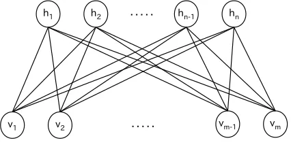
RBM is a probabilistic graphical model representing the probability distribution of training data with a fast unsupervised learning.
one hidden, that respectively have visible units (v1, v2,· · · , vm) and hidden units (h1, h2,· · · , hn) connected to each other between the two layers (Fig-ure 1).
Figure 1: Restricted Boltzmann machine.
Given training data, the weights of the connec-tions between units are modified by learning so that the behavior of the RBM stochastically fits the train-ing data as well as possible. The learntrain-ing algorithm is briefly described below.
First, sampling is performed on the basis of con-ditional probabilities when a piece of training data is given to the visible layer using Eqs. (1), (2), and then (1) again:
P(h(k)i = 1|v(k)) = sigmoid( m !
j=1
wijvj(k)+ci) (1)
and
P(vj(k+1)= 1|h(k)) = sigmoid( n !
i=1
wijh(k)i +bj),
(2) where k (≥ 1) is a repeat count of sampling and
v(1)=vwhich is a piece of training data,wij is the weight of connection between unitsvjandhi, andbj andciare offsets for the unitsvjandhiof the visible and hidden layers. Afterkrepetition sampling, the weights and offsets are updated by
W ←W +ϵ(h(1)vT−
P(h(k+1)= 1|v(k+1))v(k+1)T),
(3)
b←b+ϵ(v−v(k+1)), (4)
c←c+ϵ(h(1)−P(h(k+1) = 1|v(k+1))), (5)
whereϵis a learning rate and the initial values ofW,
b, andcare0. Sampling with a large enough repeat count is called Gibbs sampling, which is computa-tionally expensive. A method called k-step Con-trastive Divergence (CD-k) which stops sampling after k repetitions is therefore usually adopted. It is empirically known that evenk = 1(CD-1) often gives good results, and so we setk= 1in this work. If we assume totally eepochs are performed for learningntraining data using CD-k, the procedure for learning RBM can be given as in Figure 2. As the learning progresses, the samples2 of the visible layerv(k+1)approach the training datav.
Foreach of all epochsedo Foreach of all datando
Foreach repetition of CDkdo
Sample according to Eqs. (1), (2), (1) End for
Update using Eqs. (3), (4), (5) End for
End for
Figure 2: Procedure for learning RBM.
Figure 3: Example of a deep belief network.
3.2 Deep Belief Network
Figure 3 shows a DBN composed of three RBMs for pre-training and a supervised learning device for fine-tuning. Naturally the number of RBMs is changeable as needed. As shown in the figure, the hidden layers of the earlier RBMs become the vis-ible layers of the new RBMs. Below, for
simplic-2By “samples” here we mean the data generated on the basis
ity, we consider the layers of RBMs (excluding the input layer) as hidden layers of DBN. The DBN in the figure therefore has three hidden layers, and this number is equal to the number of RBMs. Al-though supervised learning can be implemented by any method, in this work we use logistic regression. The procedure for learning the DBN with three RBMs is shown in Figure 4.
1. Train RBM 1 with the training data as inputs by the procedure for learning RBM (Figure 2)and fix its weights and offsets.
2. Train RBM 2 with the samples of the hid-den layer of RBM 1 as inputs by the pro-cedure for learning RBM (Figure 2) and fix its weights and offsets.
3. Train RBM 3 with the samples of the hid-den layer of RBM 2 as inputs by the pro-cedure for learning RBM (Figure 2) and fix its weights and offsets.
4. Perform supervised learning with the samples of the hidden layer of RBM 3 as inputs and the labels as the desired out-puts.
Figure 4: Procedure for learning DBN with three RBMs.
4 Experiments
4.1 Experimental Setup
4.1.1 Data
We formed 13 training data sets by adding differ-ent amounts of automatically gathered data and/or pseudo data to a base data set, as shown in Table 2. In the table, m300 is the base data set including 300 pieces of manually gathered data and, for ex-ample, a2400 is a data set including 2,400 automat-ically gathered pieces of data and m300, p2400 is a data set including 2,400 pieces of pseudo data and m300, and a2400p2400 is a data set including 2,400 pieces of automatically gathered data, 2,400 pieces of pseudo data, and m300. Altogether there were 100 pieces of testing data. The number of labels was 10; i.e., the training data listed in Table 2 and
the testing data have 10 labels. The dimension of the feature vectors constructed in accordance with the steps in Subsection 2.4 was 182.
m300
a300 a600 a1200 a2400
p300 p600 p1200 p2400
a300p300 a600p600 a1200p1200 a2400p2400
Table 2: Training data sets.
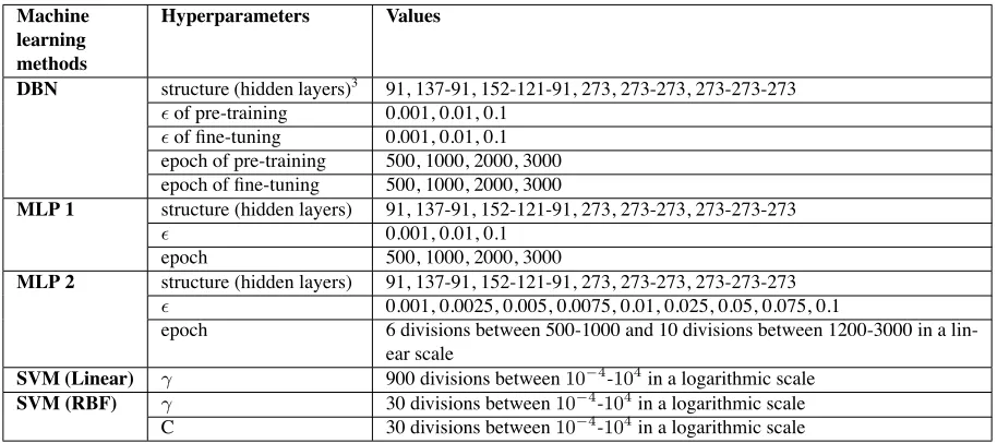
4.1.2 Hyperparameter Search
The optimal hyperparameters of the various ma-chine learning methods used were determined by a grid search using 5-fold cross-validation on training data. The hyperparameters for the grid search are shown in Table 3. To avoid unfair bias toward the DBN during cross-validation due to the DBN hav-ing more hyperparameters than the other methods, we divided the MLP and SVM hyperparameter grids more finely than that of the DBN so that they had the same or more hyperparameter combinations than the DBN. For MLP, we also considered another case in which we used network structures, learning rates, and learning epochs completely the same as those of the DBN. In this case, the number of MLP hyperpa-rameter combinations was quite small compared to that of the DBN. We refer to this MLP as MLP 1 and to the former MLP as MLP 2. Ultimately, the DBN and MLP 2 both had 864 hyperparameter combina-tions, the SVM (Linear) and SVM (RBF) had 900, and MLP 1 had 72.
4.1.3 Baselines
For comparison, in addition to MLP and SVM, we run tests on baseline methods using example-based approaches and compare the testing data of each with all the training data to determine which one had the largest number of words corresponding to the testing data. The algorithm is shown in Fig-ure 5, where the words used for counting are those extracted from the descriptive texts in accordance with steps (1)–(4) in Subsection 2.4.
Machine learning methods
Hyperparameters Values
DBN structure (hidden layers)3 91, 137-91, 152-121-91, 273, 273-273, 273-273-273
ϵof pre-training 0.001, 0.01, 0.1
ϵof fine-tuning 0.001, 0.01, 0.1 epoch of pre-training 500, 1000, 2000, 3000 epoch of fine-tuning 500, 1000, 2000, 3000
MLP 1 structure (hidden layers) 91, 137-91, 152-121-91, 273, 273-273, 273-273-273
ϵ 0.001, 0.01, 0.1 epoch 500, 1000, 2000, 3000
MLP 2 structure (hidden layers) 91, 137-91, 152-121-91, 273, 273-273, 273-273-273
ϵ 0.001, 0.0025, 0.005, 0.0075, 0.01, 0.025, 0.05, 0.075, 0.1
epoch 6 divisions between 500-1000 and 10 divisions between 1200-3000 in a lin-ear scale
SVM (Linear) γ 900 divisions between10−4-104in a logarithmic scale SVM (RBF) γ 30 divisions between10−4-104in a logarithmic scale
C 30 divisions between10−4-104in a logarithmic scale
Table 3: Hyperparameters for grid search.
Foreach inputiof testing datado Foreach inputjof training datado
1. Count the same words betweeniandj
2. Find thejwith the largest count and setm=j
End for
1. Let the label ofmof training data (r) be the predicting result of the inputi
2. Comparerwith the label ofiof testing data and determine the correctness
End for
1. Count the correct predicting results and compute the correct rate (precision)
Figure 5: Baseline algorithm.
4.2 Results
Figure 6 compares the testing data precisions when using different training data sets with individual ma-chine learning methods. The precisions are averages when using the top N sets of the hyperparameters in ascending order of the cross-validation errors, with N varying from 5 to 30.
As shown in the figure, both the DBN and the MLPs had the highest precisions overall and the SVMs had approximately the highest precision when using data set a2400p2400, i.e., in the case of adding the largest number of automatically gathered data and pseudo data to the manually gathered data as training data. Moreover, the DBN, MLPs, and SVM (RBF) all had higher precisions when adding
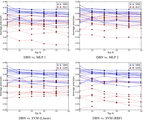
the appropriate amount of automatically gathered data and pseudo data compared to the case of using only manually gathered data, but the SVM (Linear) did not have this tendency.4 Further, the DBN and SVM (RBF) had higher precisions when adding the appropriate amount of automatically gathered data only, whereas the MLPs had higher precisions when adding the appropriate amount of pseudo data only compared to the case of using only manually gath-ered data. From these results, we can infer that (1) all the machine learning methods (excluding SVM (Linear)) can improve their precisions by adding automatically gathered and pseudo data as training data and that (2) the DBN and SVM (RBF) can deal with noisier data than the MLPs, as the automati-cally gathered data are noisier than the pseudo data. Figure 7 compares the testing data precisions of DBN and MLPs and of DBN and SVMs when us-ing different trainus-ing data sets (i.e., the data set of Table 2) that are not distinguished from each other. As in Figure 6, the precisions are averages of using the top N sets of hyperparameters in ascending order of the cross-validation errors, with N varying from 5 to 30. We can see at a glance that the performance of the DBN was generally superior to all the other machine learning methods. We should point out that the ranges of the vertical axes of all the graphs are set to be the same and so four lines of the SVM (RBF)
4This is because the SVM (Linear) can only deal with data
DBN
MLP 1 MLP 2
SVM (Linear) SVM (RBF)
DBN vs. MLP 1 DBN vs. MLP 2
DBN vs. SVM (Linear) DBN vs. SVM (RBF)
Figure 7: Comparison of average precisions for top N varying from 5 to 30.
are not indicated in the DBN vs. SVM (RBF) graph because their precisions were lower than 0.9. Full results, however, are shown in Figure 6.
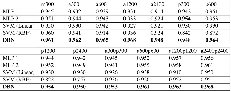
Table 4, 5, and 6 show the precisions of the base-line method and the average precisions of the ma-chine learning methods for the top 5 and 10 sets of hyperparameters in ascending order of the cross-validation errors, respectively, when using different data sets for training. First, in contrast to the ma-chine learning methods, we see that adding noisy training data (i.e., adding only the automatically gathered data or adding both the automatically gath-ered and the pseudo data) was not useful for the baseline method to improve the prediction preci-sions: on the contrary, the noisy data significantly reduced the prediction precisions. Second, in almost
all cases, the precisions of the baseline method were far lower than those of all machine learning meth-ods. Finally, we see that in almost all cases, the DBN had the highest precision (the bold figures in the tables) of all the machine learning methods.
In addition, even when only using the base data set (i.e., the manually gathered data (m300)) for training, we can conclude from Figure 6 and Table 5 and 6 that, in all cases, the precision of DBN was the highest.
5 Conclusion
learn-m300 a300 a600 a1200 a2400 p300 p600
Baseline 0.850 0.500 0.320 0.390 0.370 0.850 0.840
p1200 p2400 a300p300 a600p600 a1200p1200 a2400p2400
Baseline 0.840 0.840 0.510 0.320 0.390 0.370
Table 4: Precisions of the baseline.
m300 a300 a600 a1200 a2400 p300 p600
MLP 1 0.944 0.940 0.942 0.928 0.922 0.938 0.946
MLP 2 0.954 0.948 0.946 0.934 0.924 0.958 0.948
SVM (Linear) 0.950 0.930 0.942 0.928 0.920 0.930 0.930
SVM (RBF) 0.902 0.946 0.922 0.932 0.924 0.854 0.888
DBN 0.958 0.962 0.964 0.966 0.946 0.956 0.974
p1200 p2400 a300p300 a600p600 a1200p1200 a2400p2400
MLP 1 0.944 0.942 0.950 0.952 0.958 0.956
MLP 2 0.954 0.948 0.932 0.960 0.958 0.960
SVM (Linear) 0.930 0.930 0.920 0.940 0.940 0.950
SVM (RBF) 0.834 0.686 0.944 0.920 0.964 0.956
DBN 0.944 0.950 0.958 0.970 0.966 0.968
Table 5: Average precisions of DBN, MLP, and SVM for top 5.
m300 a300 a600 a1200 a2400 p300 p600
MLP 1 0.945 0.932 0.939 0.931 0.914 0.942 0.951
MLP 2 0.951 0.944 0.943 0.933 0.924 0.954 0.953
SVM (Linear) 0.950 0.930 0.942 0.927 0.921 0.930 0.930
SVM (RBF) 0.960 0.941 0.914 0.936 0.924 0.842 0.872
DBN 0.961 0.962 0.965 0.968 0.948 0.948 0.964
p1200 p2400 a300p300 a600p600 a1200p1200 a2400p2400
MLP 1 0.944 0.942 0.945 0.952 0.957 0.956
MLP 2 0.952 0.949 0.941 0.955 0.958 0.961
SVM (Linear) 0.930 0.930 0.926 0.938 0.940 0.950
SVM (RBF) 0.822 0.757 0.936 0.926 0.952 0.951
DBN 0.954 0.950 0.953 0.961 0.963 0.968
Table 6: Average precisions of DBN, MLP, and SVM for top 10.
ing. To determine the effectiveness of using DBN for this task, we tested it along with baseline meth-ods using example-based approaches and conven-tional machine learning methods such as MLP and SVM in comparative experiments. The data for training and testing were obtained from the Web in both manual and automatic manners. We also used automatically created pseudo data. We adopted a grid search to obtain the optimal hyperparameters of these methods by performing cross-validation on