Fast Boosting-based Part-of-Speech Tagging and Text Chunking with Efficient Rule Representation for Sequential Labeling

Fast Boosting-based Part-of-Speech Tagging and Text Chunking with

Efficient Rule Representation for Sequential Labeling

Tomoya Iwakura

Fujitsu Laboratories Ltd.

1-1, Kamikodanaka 4-chome, Nakahara-ku, Kawasaki 211-8588, Japan

[email protected]

Abstract

This paper proposes two techniques for fast sequential labeling such as part-of-speech (POS) tagging and text chunking. The first technique is a boosting-based al-gorithm that learns rules represented by combination of features. To avoid time-consuming evaluation of combination, we divide features into not used ones and used ones for learning combination. The other is a rule representation. Usual POS taggers and text chunkers decide the tag of each word by using the features gen-erated from the word and its surrounding words. Thus similar rules, for example, that consist of the same set of words but only differ in locations from current words, are generated. We use a rule representation that enables us to merge such rules. We evaluate our meth-ods with POS tagging and text chunking. The experi-mental results show that our methods show faster pro-cessing speed than taggers and chunkers without our methods while maintaining accuracy.

1 Introduction

Several machine learning algorithms such as Support Vec-tor Machines (SVMs) and boosting-based learning algo-rithms have been applied to Natural Language Processing (NLP) problems successfully. The cases of boosting in-clude text categorization [11], POS tagging [5] and text chunking [7, 5], and so on. Furthermore, parsers based on boosting-based learners have shown fast processing speed [7, 5]. However, to process large data such as WEB data and e-mails, processing speed of base technologies such as POS tagging and text chunking will be important.

This paper proposes two techniques for improving pro-cessing speed of POS tagging and text chunking. The first technique is a boosting-based algorithm that learns rules. Instead of specifying combination of features manually, we specify features that are not used for the combination of features as atomic. Our boosting algorithm learns rules that consist of features or a feature from non-atomic features, and rules consisting of a feature from atomic features.

The other is a rule representation for sequential label-ing such as POS tagglabel-ing and text chunklabel-ing. Usual POS taggers and text chunkers decide the tag of each word by using features generated from the current word and its sur-rounding words. Thus each word and its attributes, such as character-types, are evaluated several times in different relative locations from current word. We propose a repre-sentation that enables us to merge similar rules that consist of the same set of words and attributes that only differ in positions from current word.

The experimental results with English POS tagging and text chunking show the taggers and chunkers based on our methods show faster processing speed than without our methods while maintaining competitive accuracy.

2 Boosting-based Learner

2.1 Preliminaries

Let X be the set of examples and Y be a set of labels {−1,+1}. LetF = {f1, f2, ..., fM}beM types of fea-tures represented by strings.

Let S be a set of training samples

{(x1, y1), ...,(xm, ym)}, where each example xi ∈ X consists of features inF, which we call a feature-set, and

yi ∈ Y is a class label. The goal is to induce following mapping fromS:

F :X → Y.

Let |xi|(0 < |xi| ≤ M) be the number of features included in a feature-setxi, which we call the size ofxi,

andxi,j ∈ F(1≤j≤ |xi|) be a feature included inxi. We call a feature-set of sizekas ak-feature-set. We callxi is a subset ofxj, if a feature-setxjcontains all the features in a feature-setxi. We denote subsets of feature-sets as

xi⊆xj.

Then we define weak hypothesis based on the idea of the real-valued predictions and abstaining [11]. Letfbe a feature-set, called a rule,cbe a real number, called a con-fidence value, andxbe an input feature-set, then a weak-hypothesis for feature-sets is defined as

hhf,ci(x) =

½ c f⊆x

0 otherwise.

2.2 Boosting-based Rule Learning

We use a boosting-based algorithm that has shown fast training speed by treating a weak learner that learns sev-eral rules at each iteration [5]. The learner learns a final hypothesisFconsisting ofRtypes of rules defined as

F(x) =sign(PR

r=1hhfr,cri(x)).

We use a learning algorithm that generates several rules from a given training samples S = {(xi, yi)}mi=1 and weights over samples {wr,1, ..., wr,m} as weak learner.

wr,iis the weight of sample numberiafter selectingr−1 types of rules, where0<wr,i,1≤i≤mand1≤r≤R.

Given such input, the weak learner selects ν types of rules withgain:

gain(f)def=|pWr,+1(f)−pWr,−1(f)|, wherefis a feature-set, and Wr,y(f)is

Wr,y(f) =Pm_i=1wr,i[[f⊆xi∧yi=y]], where[[π]]is 1 if a propositionπholds and 0 otherwise.

The weak learner selects a feature-set having the highest

gainas the r-th rule, and the weak learner selectsνtypes of feature-sets havinggainin topνas{fr, ...,fr+ν−1}at each iteration.

Then the boosting-based learner calculates the confi-dence value of each rule in the selectedνrules and updates the weight of each sample. The confidence valuecrfor the first rulefrin the selectedνrules is defined as

##Fk: A set of k-feature-sets

##Ro:νoptimal rules (feature-sets)

##Rk,ω:ωk-feature-sets for generating candidates

##selectNBest(R,n,S,Wr): Selectnbest rules inR

## withgainon{wi,r}mi=1and training samplesS

##FN,FA: non-atomic, atomic features

procedureweak-learner(Fk,S,Wr)

##νbest feature-sets as rules

Ro=selectNBest(Ro∪Fk,ν,S,Wr);

if(ζ≤k)returnRo; ## Size constraint

##ωbest feature-sets inFkfor generating candidates Rk,ω=selectNBest(Fk,ω,S,Wr);

τ= min

f∈Rogain(f); ## Thegainofν-th optimal rule

Foreach(fk∈Rk,ω)

## Pruning candidates with upper bound of gain if(u(fk)< τ)continue;

Foreach(f∈ FN) ## Generate candidates

Fk+1= (Fk+1∪gen(fk, f)); end Foreach

end Foreach

return weak-learner(Fk+1, S, Wr);

Fig. 1:Find rules with given weights. cr=1₂log(W_Wr,_r,−1+1(₍f_fr)+r)+ε_ε),

whereε is a value to avoid to happen that Wr,+1(f) or

Wr,−1(f)is very small or even zero [10]. We setεto 1. After the calculation ofcr forfr, the learner updates the weight of each sample with

wr+1,i = wr,iexp(−yihhfr,cri(xi)). (1) Then the learner adds (fr, cr) toF as ther-th rule and its confidence value. When we calculate the confidence valuecr+1 forfr+1, we use{wr+1,1, ..., wr+1,m}as the weights of samples. After processing all the selected rules, the learner starts the next iteration. The learner continues training until obtainingRrules.

2.3 Learning Rules

We extend a weak learner that learns several rules from a small portion of candidate rules called a bucket used in [5]. Figure 1 describes an overview of the weak learner.

At each iteration, one of the |B| types of buckets is given as an initial 1-feature-setsF1 to the weak learner. We use W-dist that is a method to distributes features to|B|-buckets. To distribute features to buckets, W-dist calculates the weight of each feature that is defined as Wr(f) = Pmi=1wr,i[[{f} ⊆ xi]] (f ∈ F). ThenW-dist sorts features based on the weight of each feature, and in-sert each feature to one of the buckets.

The weak learner findsνbest feature-sets as rules from feature-sets that include one of the features in F1. The weak learner generates candidatek-feature-sets (1 < k) fromωbest (k-1)-feature-sets inFk−1withgain.

We define two types of features,FAandFN(i.eF = FA ∪ FN).FAandFNare a set of atomic features and a set of non-atomic features. When we generate candidate rules that consist of more than a feature, we only use non-atomic features inFN.

For example, if we use featuresFA ={A, B, C}and FN = {a, b, c}, we examine followings as candidates; {A},{B},{C},{a},{b},{c},{a, b},{b, c}and{a, b, c}.

Thegenis a function to generate combination of fea-tures. We denotef0_{=f+f as the generation ofk+}

1-feature-setf0_{that consists of a featurefand ak-feature-set}

f. LetID(f)be the integer corresponding tof, calledid, andφbe 0-feature-set. Then thegenis defined as follows.

gen(f, f) =

8 > < > :

φ if(f⊆ FA)

f+f if ID(f)>max

f0_∈fID(f0)

φ otherwise

.

##S={(xi, yi)}im=1: xi⊆X,yi∈ {+1}

##Wr={wr,i}mi=1: Weights of samples after learning

## r types of rules.

##|B|: The size of bucketB={B[0], ..., B[|B| −1]} ##b,r: The current bucket and rule number

##distFT: distribute features to buckets

procedureAdaBoost.SDFAN()

B=distFT(S,|B|); ##Distributing features intoB

##Initialize values and weights:

r= 1; b= 0;c0=1₂log(W_W+1₋₁);

Fori = 1,...,m:w1,i =exp(c0);

While(r≤R) ##LearningRtypes of rules

##Selectνrules and increment bucket idb

R=weak-learner(B[b], S, Wr);b++;

Foreach(f∈ R) ##Update weights with each rule

c=1

2log(WWr,r,+1−1((ff)+1)+1);

Fori=1,..,m wr+1,i=wr,iexp(−yihhf,ci(xi));

fr=f;cr=c;r++;

end Foreach

if(b==|B|) ## Redistribution of features

B=distFT(S,|B|);b=0; end if

end While

returnF(x) =sign(c0+PrR=1hhfr,cri(x))

Fig. 2:An overview of AdaBoost.SDFAN. Thegenexcludes the generation of candidates that include an atomic feature. We assign smaller integer to more infre-quent features asid. If there are features having the same frequency, we assignidto each feature with lexicographic order of features as in [4].

We also use the following pruning techniques.

•Size constraint(ζ): We examine candidates whose size is no greater than a thresholdζ.

•Upper bound of gain: The upper bound is defined as u(f)def=max(pWr,+1(f),pWr,−1(f)).

For any feature-set f0_{⊆F, which contains f (i.e.}

f ⊆ f0_{), the gain(f}0_{) is bounded under u(f), since}

0≤Wr,y(f0_)≤Wr,y(f)fory ∈ {±1}. Thus ifu(f)is less

thanτ, thegainof the current optimal rule, candidates that containfare safely pruned.

Figure 2 describes an overview of our algorithm, which we call AdaBoost for a weak learner learningSeveral rules from Distributed Features consist of Atomic and Non-atomic (AdaBoost.SDFAN, for short).1

3 Efficient Rule Representation

3.1 A Problem of Conventional Methods

When identifying the POS tags of words and chunks of words in usual parsers, we firstly generate features from current word and its surrounding words.

Let “I am happy .” be a sequence of words. If we iden-tify a tag of “am” with 3-word window, we use “I”, “am” and “happy” as features. To distinguish words that appear different locations, we usually express words with rela-tive locations from current word like “I:-1”, “am:0” and “happy:1”, where the -1, 0 and 1 after “:” are location-markers for relative locations. When “happy” is a current word, we have to express “am” as “am:-1”. Thus similar rules that differ in relative locations are generated.

3.2 Efficient Rule Representation

We propose a rule representation, calledCompressed Se-quential Labeling Rule Representation (CSLR-rep, for

1_{To reflect imbalance class distribution, we use the default rule defined}

as1

2log(WW+1−1), whereWy=

P_m

##f: a rule generated by AdaBoost.SDFAN ##sc: the score off

##cl: the class off

##s(f): the feature-stem of a featuref

##p(f): the location-marker of a featuref

##fn: the conversion result off

##RC[fn]: scores forfn procedureruleConv(f,sc,cl)

bp= min

f∈fp(f)## select the base position Foreachf∈f## generate new rule

lm=p(f)−bp## new location-marker off

## append new representation off fn=fn+ “s(f):lm”

endForeach

RC[fn] =RC[fn]∪(−bp, cl, sc)

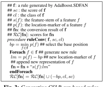
Fig. 3:Generating CSLR-rep based rules. short), to merge similar rules. To useCSLR-rep, we con-vert weak-hypotheses (WHs, for short) generated by Ad-aBoost.SDFAN toCSLR-rep. ACSLR-rep-basedWH is represented as

hrule,{(p1, cl1, c1), ...,(pq, clq, cq)}i.

Theruleis a rule generated by merging rules learned by AdaBoost.SDFAN.pp, called scoring-position, denotes the position of a word to assign a scorecpof a classclp (1≤p≤q) from current word.

We describe an example. Let h{I:−2, am:−1}, JJ, c0i , h{I:−1, am:0}, V BP, c1i and h{I:0, am:1}, P RP, c2i

be WHs generated by AdaBoost.SDFAN, and JJ,

V BP and P RP be class tags. These WHs are

converted to the following CSLR-rep-based rule;

h{I:0, am:1},{(2, JJ, c0),(1, V BP, c1),(0, P RP, c2)}i, When the convertedWHin the example is applied to a word sequence “I am happy .”, we can assign scores to all the three words by just checking{I:0, am:1}. The scores for “JJ”, “VBP” and “PRP” are assigned to “happy”, “am” and “I”, respectively.

When we use the three originalWHs in the example, we have to check three rules to assign scores to the words.

Figure 3 shows an overview for the rule conversion. We assume each feature is divided into a location-marker and a feature-stem. A location-marker is the relative location from a current word. A feature-stem is a word or one of its attributes such as character-types without a location-marker.

We use the relative location of a feature appeared in left-most word in each rule as base-position (bp, for short). Then we convert each feature to a new feature that con-sists of its feature-stem and new location-marker. The new location-marker means a relative location from thebp. We add the value of (bp×-1) as the scoring-position of the current score.

3.3 Rule Application

We describe an overview of the application of rules repre-sented byCSLR-rep. We consider two types of features, static-featuresanddynamic-features, in this application. Static-features are generated from input word sequences. Dynamic-features are dynamically generated from the tag of each word assigned with the highest score. We defineW

as a word window size that means using a current word and its surrounding words appearing W−1

2 left and W2−1 right of the current word.

Figure 4 shows an overview of the application. Let {wd1, ..,wdN}be an input that consists ofN (1 ≤ N) words. Each wordwdi(1≤i ≤N) has|wdi|types of attributes. We denotej-th attribute ofwdiaswdi,j. RC

is a set of rules represented byCSLR-repandRC[rc]is the set ofhscoring-position, class, scoreiofrc.

The application has two stages for static-features and dynamic-features. Our algorithm firstly assigns scores with rules consisting of only Static-features to each word in the direction of beginning of sentence (BOS) to end of sen-tence (EOS) direction. Rs[i]keeps the status of rule ap-plications fori-th word. If the algorithm finds a subset of rules while applying rules fromi-th word, the algorithm adds the subset of rules toRs[i]. 2 _{We define subsets of}

rules as follows:

Definition 1 Subsets of rules

If there existsruleinhrule, scoresi ∈ RCthat satisfies rc⊆rule∧rc6=rule, we callrcis a subset of rules of RCand denote it as

rc⊂ RC

Then we apply rules that include dynamic-features. All the subsets of rules are kept in Rs after examining all the Static-features, we can assign scores to words by just checking dynamic-feature of each word withRs. When checking rules that include the dynamic-feature of i-th word we check subsets of rules of words in (i−W−1

2 −∆

) to (i+max(W−1

2 ,∆) - 1). We use the tags of words with in∆in the direction of EOS.

We describe an example. LetRC={ {I:0, am:1},{I:0, VBP:1},{I:0, VBP:1, JJ:2} }be a set of rules. When ap-plying the rules to “I am happy .” with(W,∆) = (3,2), we check “I:0” first. “I:0” is inserted toRs[1]because of{I:0} ⊂ RC. Then we check “am:1” with “{I:0}” inRs[1], and{I:0, am:1}is found. Finally we check “happy:2” with Rs[1]. We check the other words like this. After checking all the words from BOS to EOS direction, we start to check rules that include dynamic-features from EOS to BOS di-rection. If the dynamic-features of “am” and “happy” are VBP and JJ, we check VBP and JJ withRs. For exam-ple, VBP is treated as “VBP:1” from the position of “I” and “VBP:0” from the position of “am”. When we check “VBP:1” with “{I:0}” inRs[1],{I:0, VBP:1}is found and inserted to Rs[1]. Then we check “JJ:2” with “I:0” and {I:0, VBP:1} inRs[1]. Then we check these dynamic-features withRs[2].

Unfortunately, theCSLR-rephas some drawbacks. One of the drawbacks is the increase of dynamic-features. When we convert rules that consist of more than a fea-ture toCSLR-rep, the number of types of dynamic-features increases. Since original rule representation only handles dynamic-features within∆, the total number of types of dynamic-features is up to “∆ ×CL”, where CLis the number of classes in each task. However, the total num-ber of dynamic-features inCSLR-rep is up to “ (W−1

2 +

∆+max(W−1

2 ,∆)-1)×CL” because we express each feature with the relative location from the base-position of each rule.

4 POS tagging and Text Chunking

4.1 English POS Tagging

We used the Penn Wall Street Journal treebank [8]. We split the treebank into training (sections 0-18), develop-ment (sections 19-21) and test (sections 22-24) as in [5]. We used the following features:

2_{We use a TRIE structure called double array for representing rules [1].}

##RC[rc]: pairs of score-positions and scores ofrc

##Rs[i]: subset of rules ofi-th word

## Initial value for each word is 0-feature-set

procedureruleApplication({wd1, ..,wdN},FN)

## For Static-feature

Fori0_{= 1;i}0_≤N;i0_{++ # beginning position} For i=i0_{;i < i+W;i++ # combination position}

For j= 1;j≤ |wdi|;j++# attributes Foreachrc∈Rs[i0_]

lm=i−i0_{## current location-marker}

rc0_{=rc+ “wdi,j:lm”} # IfRC[rc0_{]is applied,}

# assign the scores with base positioni’ assignScores(RC[rc0_],i0₎

Ifrc0_{⊂ RCRs[i}0_{] =Rs[i}0_]∪rc0 endForeach

# If no subset of rules fori0_{, go toi}0_{+ 1-th word} IfRs[i0_{] ={φ}break}

endFor endFor

## For Dynamic-feature : EOS to BOS direction Fori0_{=N; 1≤i}0_;i0_{−−# beginning position}

# Checking rules including Dynamic-feature

db=i0₋W−1

2 −∆;de=i0+max(W2−1,∆);

For i=db;i < de;i++ Foreach rc∈Rs[i]

lm=j−i0_{## current location-marker}

rc0_{=rc+ “dfti0:lm” #dftjis the tag ofi’-th word} assignScores(RC[rc0_],i)

Ifrc0_{⊂ RCRs[i] =Rs[i]∪rc}0 endForeach

endFor endFor

Fig. 4:Application of CSLR-rep based rules. ·words, words that are turned into all capitalized, in aW -word window size, tags assigned to∆words on the right. ·whether the current word has a hyphen, a number, a capi-tal letter, the current word is all capicapi-tal, all small

·prefixes and suffixes of current word (up to 4) ·candidate-tags of words in aW-word window

We collect candidate POS tags of each word, called can-didate feature, from the automatically tagged corpus pro-vided for the shared task of English Named Entity recogni-tion in CoNLL 2003 as in [5]. 3 4 _{We express these}

can-didates with one of the following ranges decided by their frequencyfq: 10 ≤ fq < 100, 100 ≤fq < 1000 and 1000≤fq.

If ’work’ is annotated as NN 2000 times, we express it like “1000≤NN”. If ’work’ is current word, we add 1000≤NN as a candidate POS tag feature of the current word. If ’work’ appears the next of the current word, we add1000≤NN as a candidate POS tag of the next word.

4.2 Text Chunking

We used the data prepared for CoNLL-2000 shared tasks.5

This task aims to identify 10 types of chunks, such as, NP, VP and PP, and so on. The data consists of subsets of Penn Wall Street Journal treebank: training (sections 15-18) and test (section 20). We prepared the development set from section 21 of the treebank as in [5].6

Each base phrase consists of one word or more. To iden-tify word chunks, we useIOE2representation. The chunks are represented by the following tags: E-X is used for end word of a chunk of class X. I-X is used for non-end word in an X chunk. O is used for word outside of any chunk.

3_{http://www.cnts.ua.ac.be/conll2003/ner/}

4_{We collected POS tags for each word that are annotated to the word}

more than 9 times in the corpus as candidates.

5_{http://lcg-www.uia.ac.be/conll2000/chunking/}

6_{We usedhttp://ilk.uvt.nl/˜sabine/chunklink/chunklink 2-2-2000 for conll.plfor creating}

de-velopment data.

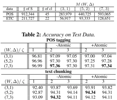
Table 1: Training data for experiments. POS and ETC indicate POS tagging and text chunking.]of S,]of cl and

M indicate the number samples, the number of class in each data set and the distinct number of feature types for each pair of (W,∆).

M(W,∆) data ]of S ]of cl (3,1) (5,2) (7,3)

POS 912,344 45 283,979 440,725 593,065 ETC 211,727 22 56,917 93,333 128,651

Table 2:Accuracy on Test Data.

POS tagging

-Atomic +Atomic

(W,∆)/ ζ 1 2 3 2 3

(3,1) 96.81 97.09 97.05 97.00 97.04

(5,2) 96.96 97.30 97.30 97.25 97.28

(7,3) 96.99 97.36 97.30 97.31 97.34

text chunking

-Atomic +Atomic

(W,∆)/ ζ 1 2 3 2 3

(3,1) 92.40 93.87 93.69 93.91 93.82

(5,2) 92.87 94.31 94.14 94.34 94.31

(7,3) 93.09 94.32 94.11 94.12 94.11

For instance, “[He] (NP) [reckons] (VP) [the current ac-count deficit] (NP)...” is represented by IOE2 as follows; “He/E-NP reckons/E-VP the/I-NP current/I-NP account/I-NP deficit/E-account/I-NP”.

We used the following features:

·words and POS tags in aW-word window. ·tags assigned to∆words on the right. ·candidate-tags of words in aW-word window.

We collected the followings as candidate-tags for chunking from the same corpus used in POS tagging.

• Candidate-tags expressed with frequency information as in POS tagging

• The ranking of each candidate decided by frequencies in the automatically tagged data

• Candidate tags of each word

If we collect “work” annotated as I-NP 2000 times and as E-VP 100 times, we generate the following candidate-tags for “work”; 1000≤I-NP,100≤E-VP<1000, rank:I-NP=1 rank:E-NP=2, candidate=I-NP and candidate=E-VP.7

5 Experiments

We testedR=200,000,|B|=1,000,ν= 10,ω=10,ζ={1,2,3} and(W,∆)={(3,1), (5,2), (7,3)}. Table 1 shows that the number of training samples, classes, features.

We examine two types of training, “-Atomic ” and “ +Atomic ”, in this experiment. “-Atomic ” indicates traing with all the features as non-atomic. “ +Atomic ” in-dicates training by using atomic features. We specify pre-fixes, suffixes and candidate-tags as atomic for POS tag-ging, and candidate-tags as atomic for text chunking.

To extend AdaBoost.SDFAN to handle multi-class prob-lems, we used the one-vs-the-rest method. To identify proper tag sequences, we use Viterbi search.8

5.1 Tagging and Chunking Accuracy

Table 2 shows accuracy obtained with each rules on POS tagging and text chunking. We calculate label accuracy for 7_{We converted the chunk representation in the corpus to IOE2 and we}

collected chunk tags of each word appearing more than 9 times.

8_{We map the confidence value of each classifier into the range of 0 to 1}

with sigmoid function defined ass(X) = 1/(1+exp(−βX)), where

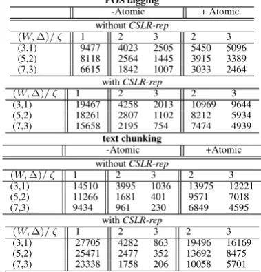
Table 3: Tagging and Chunking Speed. Each number is average processed words per second. We examine three times measurements for each tagger or chunker. Each time is obtained with all rules.

POS tagging

-Atomic + Atomic

withoutCSLR-rep

(W,∆)/ ζ 1 2 3 2 3

(3,1) 9477 4023 2505 5450 5096

(5,2) 8118 2564 1445 3915 3389

(7,3) 6615 1842 1007 3033 2464

withCSLR-rep

(W,∆)/ ζ 1 2 3 2 3

(3,1) 19467 4258 2013 10969 9644

(5,2) 18261 2807 1102 8212 5934

(7,3) 15658 2195 754 7474 4939

text chunking

-Atomic +Atomic

withoutCSLR-rep

(W,∆)/ ζ 1 2 3 2 3

(3,1) 14510 3995 1036 13975 12221

(5,2) 11266 1681 401 9571 7018

(7,3) 9434 961 230 6849 4595

withCSLR-rep

(W,∆)/ ζ 1 2 3 2 3

(3,1) 27705 4282 863 19496 16169

(5,2) 25471 2477 352 13692 8475

(7,3) 23338 1758 206 10058 5701

POS tagging as accuracy. As for text chunking, we calcu-late F-measure (Fβ=1) given by2rp/(r+p)as accuracy, whererandpare recall and precision. Each accuracy on a test data is calculated with the number of rules that show the best accuracy on development data.

We obtain almost the same accuracy even if we use part of features as atomic.

5.2 Tagging and Chunking Speed

Table 3 shows tagging and chunking speed. We measure the number of words processed by per second.9 _We

ob-tain faster processing speed by usingCSLR-rep-based rules traind withζ = {1,2}and - Atomic. These show that CSLR-repcontributes to improved processing time. When we use rules trained withζ= 1, we can get more improve-ment than using rules trained withζ= 2.

However, the performance obtained with CSLR-rep -based rules trained with (ζ = 3,−Atomic) is slower than with the original rules. We guess this is caused due to the following two reasons. OurCSLR-repreduces the number of times of rule evaluation up to1/W . ThusCSLR-rep reduces processing time linearly. However, the number of combination of features exponentially increases. The other reason is that the number of times to generate dynamic-features is increased as described in the end of section 3.3. We obtain much improvement by using atomic features withCSLR-rep. For example, processing speed obtained with the text chunker using rules (ζ= 3, W = 7, +Atomic) is about 28 times faster than the speed obtained with the chunker using rules (ζ= 3, W = 7, -Atomic ).

6 Related Work

We list previous best results on English POS tagging and Text chunking in Table 4. The tagger and chunker based on AdaBoost.SDFAN show competitive F-measure with pre-vious best results.

9_{We used a machine with 3.6GHz DualCore Intel Xeon and 10 GB}

memory.

Table 4:Comparison with previous best results.

POS tagging Guided learning [12] 97.33

Boosting [5] 97.32

CRF [13] 97.40

This paper 97.34

Text Chunking LaSo [2] 94.4 Boosting [5] 94.30 CRF [13] 95.15 This paper 94.34

As for fast classification methods, techniques for con-verting or pruning models or rules generated by machine learning algorithms are proposed. Model conversion tech-niques for SVMs with polynomial kernel that converts kernel-based classifier into a simple liner classifier are pro-posed in [3, 6]. For AdaBoost, a pruning method for hy-potheses is proposed in [9].

Our method uses a rule conversion technique for sequen-tial labeling problems. Although CSLR-repcan only be used in tasks that use each word as different features time and again, such as POS tagging and text, we obtain faster processing speed without loss in accuracy.

7 Conclusion and Future Work

We have proposed techniques for fast boosting-based POS tagging and text chunking. To reduce time-consuming rule evaluation, our method controls the generation of combi-nation of features by specifying part of features that are not used for combination. We have also proposed a rule rep-resentation that enables us to merge similar rules. Experi-mental results have showed our techniques improve classi-fication speed while maintaining accuracy.

References

[1] J. Aoe. An efficient digital search algorithm by using a double-array structure. InIEEE Transactions on Software Engineering, volume 15(9), 1989. [2] H. Daum´e III and D. Marcu. Learning as search optimization: approximate

large margin methods for structured prediction. InProc. of ICML 2005, pages 169–176, 2005.

[3] H. Isozaki and H. Kazawa. Efficient Support Vector classifiers for named entity recognition. InProc. of COLING 2002, pages 390–396, 2002. [4] T. Iwakura and S. Okamoto. Fast training methods of boosting algorithms for

text analysis. InProc. of RANLP 2007, pages 274–279, 2007.

[5] T. Iwakura and S. Okamoto. A fast boosting-based learner for feature-rich tagging and chunking. InProc. of CoNLL 2008, pages 17–24, 2008. [6] T. Kudo and Y. Matsumoto. Fast methods for kernel-based text analysis. In

Proc. of ACL-03, pages 24–31, 2003.

[7] T. Kudo, J. Suzuki, and H. Isozaki. Boosting-based parse reranking with sub-tree features. InProc. of ACL 2005, pages 189–196, 2005.

[8] M. P. Marcus, B. Santorini, and M. A. Marcinkiewicz. Building a large anno-tated corpus of english: The Penn Treebank. pages 313–330, 1994. [9] D. D. Margineantu and T. G. Dietterich. Pruning adaptive boosting. InProc.

of ICML 1997, pages 211–218, 1997.

[10] R. E. Schapire and Y. Singer. Improved boosting algorithms using confidence-rated predictions.Machine Learning, 37(3):297–336, 1999.

[11] R. E. Schapire and Y. Singer. Boostexter: A boosting-based system for text categorization.Machine Learning, 39(2/3):135–168, 2000.

[12] L. Shen, G. Satta, and A. Joshi. Guided learning for bidirectional sequence classification. InProc. of ACL 2007, pages 760–767, 2007.