The calibration of fluid-object interaction in immersed boundary
method
Martin Buˇs´ık,IvanCimr´ak
Cell-in-fluid research group, University of ˇZilina, Slovakia, [email protected]
Abstract. In modelling of elastic objects immersed in a fluid, very important part of the model is the inter-action between objects and fluid. In models based on immersed boundary method and lattice-Boltzmann method, this interaction is mediated by friction coefficient between fluid and particles. The friction coeffi-cient is phenomenological and needs to be properly calibrated. In this work we design an experiment, the results of which can be predicted by theoretical computations. Based on the theory, we calibrate friction coefficient to properly describe the interaction between fluid and objects. The simulation experiments are performed in Object-in-fluid framework. We calibrate it for objects immersed in flow with low Reynolds number to model flow of cells inside microfluidic devices. We analyze dependence of interaction method on number of nodes and size of spherical object.
1 Introduction
We consider model of elastic objects immersed in a fluid based on the lattice-Boltzmann (LB) method coupled with the immersed boundary (IB) method. Both methods have its own mesh, one for the fluid and one for the object.
In the LB method, fluid is modeled by fictive parti-cles that travel and collide over a fixed cubic lattice mesh [?]. The fluid dynamics are computed using the LB equa-tion. The unknown variable in this equation is the density function for the fictive particles. Macroscopic properties of the fluid can be afterwards recovered from the density function.
In the IB method, the objects are characterized by tri-angulation of their surface. The discretization mesh con-tains boundary points linked together by elastic forces along the edges and faces of the mesh. These forces move the IB points in the space according to Newton equation of motion. This equations include the mass of individual IB points. This way, the object’s boundary may change the shape according to the elastic forces. The IB mesh is not fixed, the positions of the IB points are determined freely in the space.
To maintain mechanical properties of the cell’s mem-brane, five elastic moduli are considered, each defining different forces. These moduli govern the stretching and bending of the membrane, as well as local and global preservation of the surface and volume of the cell.
The interaction between the fluid and the object is provided by coupling of LB and IB method. From the fluid velocity field given over the LB fixed mesh, the cor-responding fluid forces are applied to IB points, adding up with elastic forces. Reversely, the change of object’s shape generates forces that are applied back to the fluid by en-tering the external forces in the governing LB equation
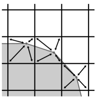
for the LB method. Since the fixed LB mesh and free IB mesh do not overlap, we need to interpolate the values of respective forces and velocities between the IB points and the lattice points as depicted in Figure??.
Fig. 1. Two dimensional version of the LB-IB method cou-pling. The respective forces and velocities are transferred from and to the vertices of LB lattice squares where the IB point is currently located.
In our case, we use transfer force between the objects and the fluid similarly as in [?] by following equation
Fi=ξ(vi−ui), (1)
whereviis the velocity of the IB pointi,ui is the interpo-lated velocity of the fluid at the particle positioni andξ is phenomenological friction coefficient. Then, total force exerted on each IB mesh point consists of elastic forces and force of fluid-object interaction [?].
Current implementation of the Object-in-fluid frame-work distributed as a part of ESPResSo [?] requires to set the friction coefficient. This phenomenological con-stant was previously calibrated by the following experi-ment: A rigid ball with the same density as surrounding fluid was put into a static fluid. The ball was pushed with given nonzero initial velocity. The resulting drag force of the fluid on the sphere may be computed explicitely. This drag force slows the sphere down and the velocity evolu-tion of the sphere may be evaluated by theoretical compu-tations. The computational simulations of this experiment were performed using the Object-in-fluid framework and the corresponding friction coefficient was determined to fit the theoretical data [?].
The computational experiment however was performed according to the authors not correctly. The initial speed of the sphere was set to the IB points only and the inner fluid of the sphere was initiated with zero speed. This way, the whole movement had to be mediated by the IB points only, while we argue that the inner fluid should have been initiated with the same initial speed as the IB points.
The remedy for this situation is however not trivial. In the LB method, setting the nonzero initial speed to inner LB points of the sphere while preserving zero speed to the neighbouring outer LB lattice points, is unphysical and leads to shocks. Therefore we present new experiment with physically correct assumption in Section??.
1.1 Theoretical considerations
In general, the motion of any object under the application of given force, is described by the Newton’s second law of motion
F =mv, (2)
where m is the mass of the object and v is the acceler-ation of the object. We consider small solid rigid sphere relatively slow speed. The drag force of the fluid exerted on moving objects with very low Reynolds number (Re<1) is described by Stoke’s law as
Fd= 6πνrKv, (3)
whereris the radius of the object,vis the relative veloc-ity of the object to the fluid, K is the shape dependent constant, for spherical objectK= 1,andνis the dynamic viscosity of the fluid. This equation assumes the object to be immersed in an unbounded fluid. Otherwise, complex boundary effects will come into play.
2 Simulation setup
Based on the previous theoretical considerations, we de-signed the following simulation experiment.
2.1 Terminal velocity experiment
We put a spherical object into a static flow. We exert a horizontal constant forceF0 on the sphere that causes the sphere to move horizontally. The static fluid will reversely exert a drag force on the sphere. As mentioned above, the drag force is directly proportional to the velocity of the sphere. Therefore the drag force is increasing and we can compute the velocity profile.
The Newton equation of motion for such sphere is
mv =F
0−6πνrv. (4)
This differential equation has the following solution
v(t) = F0 6πνr−
F0 6πνrexp
−6πνrt m
. (5)
We can see that the velocity depends on the mass of the sphere. In the coupled LB-IB method, there is fluid contributing to the object’s mass as well as the mass of IB points. There is however no direct way how to interpret the physical object’s mass in terms of model components (LB fluid mass and IB points mass).
We can however get rid of the object’s mass in the velocity expression by considering the terminal velocity as limitt→ ∞
v∞= lim
t→∞v(t) =
F0
6πνr, (6)
wherev∞is terminal velocity. This way we do not have the problem with overall mass of the object, since the terminal velocity do not depend on the object’s mass.
When simulating this experiment, we obtain terminal velocity of the simulated sphere that should be the same as in (??). This will however hold true only if the inter-action between fluid and object is calibrated properly. In other ways, the simulated terminal velocity will equals to theoreticalv∞ only if the friction coefficient is correct.
2.2 Restriction on practical implementation
2.3 Implementation details
We simulate experiments by software ESPResSo with frame-work Object-in-fluid. It allows to simulate elastic object described by triangulation its surface filled with the same fluid as outside. The simulation box has a cubical shape with uniform discretization. The discretization grid is cho-sen such that we do not have significant boundary effects. The boundary conditions for the fluid on the all sides of the simulation box are set to be zero.
Every time a particular force must be exerted on a spherical object, this force is divided by the number of IB mesh points and only afterwards it is applied to each IB point.
We use different meshes with different number of nodes, lengths of edges and sizes of the object. All meshes how-ever are quasi-uniform in a sense that they are composed of almost equilateral triangles.
Since the model we are working with is primarily used for elastic objects, we set quite high elastic coefficients to ensure that simulated object behaves like a rigid one. To control this effect we record the differences in the volume, surface area and maximal diameter of the object at the beginning and at the end of the simulation. We keep all these differences under the threshold 5%.
3 Computational analysis and results
3.1 Size of the simulation box
Theoretical considerations in Section ?? assume the im-mersed sphere in a unbounded fluid to eliminate boundary effects. In practice, we need to set up the simulation box large enough so that boundary effects are negligible. We follow the numerical simulation reported in [?] where the ratio between the size of the sphere and the simulation box was approximately 1:30. With the size of our sphere having diameter 8μmwe set the size of the box to 200μm. Moreover we perform an analysis of the influence of the simulation box on the resulting drag force.
Setting the friction coefficient to 1.0 we choose four different sizes of cubic box: 50μm, 100μm, 200μm and 400μm. We perform the simulation for the terminal veloc-ity. The results are presented in Table??.
Table 1. Terminal velocities for different box sizes for fixed friction coefficientξ= 1.0
s(size of box) 50μm 100μm 200μm 400μm vs (term. vel.) 0.00304 0.00356 0.00381 0.00395 δs→2s (rel. diff.) +14.61% +6.56% +3.54%
The differences reported in Table ?? are defined as relative difference when doubling the size of the box by expression
δs→2s= v2s−vs v2s
We can see that the differences between the terminal velocities when changing the size of the box from 200μmto 400μmis less then 5%. Therefore we will perform all sub-sequent simulation using the size of simulation box 200μm.
3.2 Results for fixed mesh and fixed size of the sphere
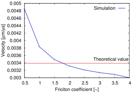
Although we assume that the friction coefficient will change for different triangulations, first we determined the friction coefficient for mesh with 393 points and with radius 4μm. We set density of fluid to 1025kg.m−3, dynamic viscosity to 1.5375×10⁻³P a.sand force exerted on the sphere to 0.393×10⁻⁹N. We performed a series of simulations of terminal velocity experiment described in Section??. We varied the value of friction coefficient and for each value we obtained different terminal velocity. In Figure ??we can see the results with value of friction coefficient computed from theoretical consideration indicated by red horizontal line. The intersection of the line and the curve determines the calibrated friction coefficient with value 1.76. In the
0.003 0.0032 0.0034 0.0036 0.0038 0.004 0.0042 0.0044 0.0046 0.0048 0.005
0.5 1 1.5 2 2.5 3 3.5 4
Theoretical value
Velocity [
μ
m/
μ
s]
Friciton coefficient [−] Simulation
Fig. 2. The dependence of friction coefficient on the terminal velocity experiment.
figure we can see that the terminal velocity is more sensi-tive for lower values of friction coefficients and increasing the friction coefficient above certain level does not influ-ence the terminal velocity much.
3.3 The dependence of friction coefficient on the number of nodes and radius of the sphere
Heuristics
First we analyze situation for two different meshes with number of mesh points n1 and n2 with the radius of the sphere fixed. We want to find out what is the relation between corresponding friction coefficients ξ1 and ξ2 in order to achieve the same simulated behaviour.
As soon as the sphere reaches terminal velocity, all forces exerted on the mesh points come to equilibrium. There are three types of forces exerted on the mesh points: elastic forces, dragging forceF0, and fluid forces that act in the opposite direction to F0. The elastic forces just keep the sphere almost solid and do not contribute to the balance between the dragging force and the fluid force. So basically, in each mesh point we have the equilibrium of the dragging force and the fluid force. We can use (??) to calculate the fluid force and thus we have for both meshes
F0=
n1
i=1
ξ1(ui−vi) = n2
i=1
ξ2(ui−vi). (7)
Our aim is to get the same behaviour of simulated sphere in the computational experiment and thus the velocities ui of mesh points for both meshes will be the same. The same holds for the fluid interpolated velocitiesviand thus
we can conclude that
n1
i=1
ξ1=
n1
i=1
ξ2, or n1.ξ1=n2.ξ2. (8)
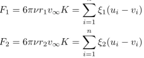
Second, we analyze the situation when we keep the number of mesh points fixed equal ton and we have two different radii r1 and r2. Assume that we want to use two different dragging forces F1 and F2 to get the same terminal velocity for both spheres. In the equilibrium, the dragging forcesF1, F2 are compensated by the drag force computed from (??) and thus we get
F1= 6πνr1v∞K=
n
i=1
ξ1(ui−vi)
F2= 6πνr2v∞K=
n
i=1
ξ2(ui−vi)
With similar argumentation as before we note that both spheres are moving with the same terminal velocity and thusuiandviare the same. Using this result after dividing the previous two equations we end up with
r1
r2 =
n.ξ1
n.ξ2 =
ξ1
ξ2 (9)
Hypotheses
From relations (??) and (??) that we have obtained using heuristic considerations, we can formulate the following two hypotheses:
(a) the friction coefficient increases linearly with the increasing radius of the sphere
(b) the friction coefficient decreases linearly with the increasing the number of nodes
Both hypotheses may be merged into one expression. Starting from the already calibrated value of friction co-efficient ξ393,4 for mesh with 393 nodes and radius 4μm, we can write down the following expression for mesh with nnodes and radius of spherer
ξn,r =393
n r
4ξ393,4. (10)
This expression reflects both hypotheses and satisfies both (??) and (??).
Verification
To confirm these hypotheses, we performed number of simulations. We picked 4 different meshes with number of nodes 126, 393, 500, 1182. With each mesh we consid-ered three different radii 2, 4 and 8μm. For each of these 12 cases we computed the friction coefficient using (??). Then we performed our computational experiment with fixedF0and we recorded the obtained terminal velocities. In first two columns of Table ?? we can see the pa-rameters of the simulations. In column 3 we see values of friction coefficient computed from (??). In next column we see the obtained terminal velocity that can be compared to the theoretical value of terminal velocity computed from (??) presented in column 5. In the last column we can see relative error in v∞.
The relative error in all simulations is low (under 5%) which confirms the validity of (??).
Table 2.The comparative result for different radiui and num-ber of mesh points. The calibrated case is emphasized with boldface.
mesh r ξ vsim vexact δsim→exact
126 2 2.74 0.006532 0.006780 3.66 % 126 4 5.49 0.003428 0.003390 1.10 % 126 8 10.89 0.001668 0.001695 1.60 % 393 2 0.88 0.006532 0.006780 0.72 %
393 4 1.76 0.003404 0.003390 0.41 %
393 8 3.52 0.001646 0.001695 2.89 % 500 2 0.69 0.006515 0.006780 3.92 % 500 4 1.38 0.003399 0.003390 0.26 % 500 8 2.77 0.001645 0.001695 2.98 % 1182 2 0.29 0.006513 0.006780 4.18 % 1182 4 0.59 0.003400 0.003390 0.30 % 1182 8 1.17 0.001644 0.001695 3.01 %
4 Summary and discussion
mesh points. This formula was confirmed by series of com-putational simulations.
The results presented in Table ?? indicate two phe-nomena. First, when keeping the radius fixed to value 4μm for which the friction was calibrated, the relative error be-tween simulated and exact terminal velocity is very low, under 1%. This suggests, that the change of the mesh den-sity with size of the object fixed is a safe operation.
Second, when keeping the number of mesh points fixed and changing the radius, relative errors are bit higher, but still acceptable. This indicate that the behaviour of the sphere is more sensitive to the changes in mesh density.
References
1. P. Ahlrichs, B. Dunweg, Lattice-Boltzmann simulation of polymer-solvent systems, Internat. J. Modern Phys. C vol. 8 (1998) 1429 - 1438
2. I. Cimr´ak, M. Gusenbauer, T. Schrefl, Modelling and simu-lation of processes in microfluidic devices for biomedical ap-plications, Computers and Mathematics with Applications vol. 64 (2012) 278 - 288
3. I. Janˇcigov´a, Modeling elastic objects in fluid flow with biomedical applications, Dissertation Thesis, Faculty of Man-agement Science and Informatics, University of ˇZilina, 2015 4. B. Dunweg and A. J. C. Ladd, Lattice-Boltzmann simula-tions of soft matter systems, Advances in Polymer Science, vol. 221 (2009) 89–166
5. D. A. Jones and D. B. Clarke, Simulation of Flow Past a Sphere using the Fluent Code, Maritime Platforms Division, Defence Science and Technology Organisation, DSTO-TR-2232, AR-014-365, 2008
6. A. Arnold, O. Lenz, S. Kesselheim, R. Weeber, F. Fahren-berger, D. Roehm, P. Koovan, and C. Holm, ESPResSo 3.1 - molecular dynamics software for coarsegrained models, in Meshfree Methods for Partial Differential Equations VI, Lec-ture Notes in Computational Science and Engineering, M. Griebel and M. Schweitzer, Eds., vol. 89, 2013, pp. 123. 7. I. Janˇcigov´a, On mass distribution in ESPResSo simulations