The equilibrium gap method : a two-scales approach
F. Amiot1,a
FEMTO-ST Institute, CNRS-UMR 6174/UFC/ENSMM/UTBM, 24 chemin de l’ ´Epitaphe, F-25030 Besanc¸on, France
Abstract. Optical full-field measurement methods are increasingly used in the field of experimental mechanics, and several techniques have been developped to make the most of the redundancy of the measured fields. However, the number of modelling parameters that can be retrieved is strongly connected to the noise level corrupting the measured fields. Focusing on the techniques based on the construction of a statically admissible field from the experimental data, a two-scales approach is proposed. It relies on the fact that, using a finite-element description of the struture, the larger the number of degrees of freedom to be measured, the more degraded by noise. It is therefore proposed to use displacement fields measured at two different scales. This paper describes the way the macro displacement fields basis is built.
1 Introduction
Optical full-field measurement methods are increasingly used in the field of experimental mechanics. These techniques are now well established so that extensive knowledge about the mechanisms driving the measurements quality is now available (for DIC measurements, see [1]). These methods provide a very large amount of data, so that different techniques have been proposed to identify material prop-erties using redundant or full-field kinematic data [2]. However, the number of parameters that can be identified using these methods is directly related to the noise level degrading the measured field. This can lead to either significant errors on the description or a poor resolution of the structure un-der scrutiny, especially when this is extremely heterogeneous and/or subjected to an unknown loading field (i.e. for MEMS devices [3]). The equilibrium gap method is first recalled, before a two-scales approach is presented. The projection conditions to be satisfied by the macro displacement field basis are then derived, and a procedure to build the projection operator is proposed. The method is then illustrated on an example.
2 Mono-scale equilibrium gap method
One considers an elastic body, whose displacement is measured at several points x. For the sake of brevity, only cantilever beams under transverse loading are considered in the sequel. One supposes a stiffness field C(x) described by a finite number of functions di(x) and a scaling parameter C0:
C(x)=C0
N
X
i=1
Didi(x) (1)
where N is the number of used functions and{Di}i=1...N the projection of the stiffness field onto the
defined basis. The structure is subjected to a loading field Qm(x), which is also described by a finite
a e-mail:[email protected]
© Owned by the authors, published by EDP Sciences, 2010
numberS of functionsψms(x)
Qm(x)= S
X
s=1
Fmsψms(x) (2)
{Lms}s=1...S is the projection of the loading field onto the defined basis. This results in a out-of-plane displacement fieldvm(x) :
vm(x)= K
X
k=1
Umkφmk(x) (3)
In the following, it will be assumed that the chosen basis are well suited to describe both stiffness, loading and displacement fields. The previously proposed equilibrium gap method ([5]) then relies on the finite element formulation of the direct problem : when the stiffness and loading fields are known (through their projectionsDandLm), the nodal displacement componentsUmkare computed by solving
KmUm=Lm (4)
The components of the stiffness operatorKmread
Kmk,l =C0
N
X
i=1
Di
Z di(x)
d2φ
mk(x) dx2
d2φ
ml(x)
dx2 dx (5)
and
Lmk =
S
X
s=1
Fms
Z
ψms(x)φmk(x)dx (6)
In order to identify the fieldsC(x) andQm(x) from measured displacement fields, and contrary to the resolution of the direct problem, the nodal displacement fieldUm is here considered as “almost” known (i.e.,measured)
Um≃Ucm (7)
The equilibrium conditions (4) are then recast as
Mm
c Um
S=Km(S)Ucm−Lm(S)=R (8)
whereSis the concatenation of the stiffness parametersDand the loading parametersFm. The Eq.(8) is solved for the non-trivialSby minimization of the residualRwhen the number of nodal displacements used to write the equilibrium conditions is large compared to the number of parameters to identify. When the number of unknowns inSincreases, the Eq.(8) is solved by singular value decomposition taking into account that under the assumption of linear behavior, the operatorMm is singular, and the solutionSsolis obtained as the right singular vector associated to the least singular value [3]. The sensitivity of this last procedure to the measurement noise has been assessed and has been found to dramatically increase with the number of parameters to be identified, therefore limiting, for a given measurement quality, the achievable description level. This is a critical issue when the structures and/or the loadings are not well defined, for example when dealing with MEMS devices under environmental loadings.
Equation (8) then defines a statically admissible displacement field. Any norm of the residualR then provides a distance between the measured displacement field and its statically admissible pro-jection. From its definition, finding a statically admissible displacement field is similar to finding the stiffness and the loading related by this statically admissible displacement field.
3 Two-scales approach
3.1 Projection conditions
using different projections of the measured displacement field onto different basis, thus defining a “macro”-measured displacement fieldvM(x) :
vM(x)= P
X
p=1
UMpφMp(x) (9)
withP<K. For a given structure, described by the sets{Dn,Lms}, it is then worth noting that one has two ways of computing the displacement projection{UMp}:
– The first one mimics the projection of the measured displacement field onto the reduced kernel of displacement functions. The displacement fieldvm(x) is computed using the equilibrium condi-tions at the micro-scale (Eq. (4)) and projecting the obtained displacement field onto the “macro” displacement basis.
– The second way involves an homogenization procedure. Using a suitable macro stiffness matrix KM, the macro displacement fields satisfies some macro equilibrium conditions :
KMUM=LM (10)
If the first way would be natural from the computing point of view, it is useless from the experimental one since it requires unachievable data. The problem is then to define some conditions on the basis to be used so that the second way will provide the same projected displacement field than the first way.
Let us define the projection operatorWso that the function basis at the macro and micro scales are related through
φMp(x)= K
X
k=1
Wpkφmk(x) (11)
Wis therefore defined byP×Kcoefficients. Starting with the first way, the displacement field at the macro scaleUk⋆
M derived from a test displacement field at the micro scaleU⋆m is simply obtained by projection onto the macro basis. Minimizing a least-square norms yields
WH WtUkM⋆=AMUkM⋆=WHU⋆m (12)
whereHis defined by
Hi j=
Z
φmi(x)φm j(x)dx (13)
On the other hand, the stiffness matrix at the macro scaleKMis obtained by expressing the strain energy in the micro stiffness field and the macro displacement field. The definition (11) then yields
KM=WKmWt (14)
The macro loading termLM is also obtained by writing the work of the micro loading field in the macro displacement field
LM=WLm=WKmU⋆m (15)
The displacement field at the macro scaleUs⋆
M is therefore defined as satisfying
KMUsM⋆=LM (16)
The displacement fieldUk⋆
M is the one that is measured when using a reduced functions kernel (that is with a reduced noise sensitivity), whereasUs⋆
M satisfies the equilibrium conditions at the macro scale as long as these are satisfied at the micro scale. Finding an operatorWso that
Uk⋆
allows one to get equilibrium conditions at the macro scale (on the parameters at the micro scale) from displacement fields measured at the macro scale, so that these are less corrupted by the measurement noise. The condition (17) then yields
WKm
WtA−M1WH − IUm=WKm·Gm=0 (18)
The condition (18) is satisfied for any stiffness field ifGmbelongs to stiffness operator nullspaceKm⊥. As the stiffness operator is obtained without use of any a priori boundary condition on the displacement (since the latter are measured),K⊥
m is composed of the structure rigid-body motions. It is therefore straightforward to define the operatorR⊥so that
Rt⊥·Gm =0 (19)
One therefore has to define the projection operatorWsatisfying Eq.(19) for some user-defined test displacement fieldsU⋆
m.
3.2 Projection operator computation
Considering the singular value decomposition ofH
H =VEVt (20)
the projection operatorWis sought as
W=PVt (21)
The problem turns then to find the operator
G=PtPEPt−1P (22)
satisfying
VGEVtU⋆
m=U⋆m+Rr0 (23)
whereRr0is a linear combination of the rigid body motions subspace. DefiningGthrough its singular
value decomposition
G=VsDsVts (24)
Vsis orthogonal,Dsis diagonal, and a solution reads
P=Vts (25)
provided that
VtsEVs=D−s1 (26)
Focusing on cantilever beams under flexure loading,Vscan be computed using a single test displace-ment fieldU⋆
m. Defining
Z1=
EVtU⋆ m kEVtU⋆ mk
(27)
Z2(r0)=
Vt U⋆
m+Rr0−Zt1Vt U⋆m+Rr0Z1 kVt U⋆
m+Rr0−Zt1Vt U⋆m+Rr0Z1k (28)
the problem turns to findγandr0so that
Vts=
" cos(
γ) sin(γ) −sin(γ) cos(γ)
# " Zt
1
Zt
2(r0)
#
satisfies Eq.(22) under the constrain defined by Eq.(26). It can be proved that the set
r0=0 (30)
γ= 1 2tan
−1 2Z2(0)tEZ1
Zt
1EZ1−Z2(0)tEZ2(0)
!
(31)
satisfies Eq.(22) and Eq.(26). The above described procedure can be repeated to allow Eq.(23) to be satisfied byP
2 distinctU⋆mtest displacement fields, considering orthogonal subspaces. It’s worth noting the strain energy computed from the micro and macro displacement fields are then equal for the chosen U⋆
m.
3.3 Example
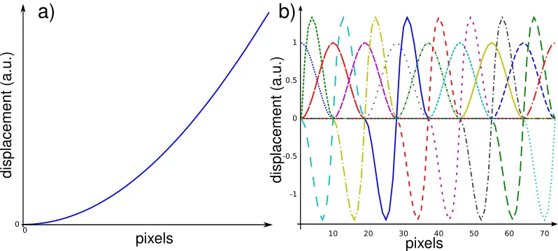
The above described procedure is illustrated using a cantilever beam meshed by 8 elements on which the displacement is projected onto cubic Hermite functions (four degrees of freedom per element). The cantilever is clamped at one end and is free at the other. Numbering the elements fromn= 1 to n=8 when moving from the clamping to the free end, the stiffness is assumed to be constant on each element and to linearly decrease when moving away of the clamping, so that the bending stiffness of the elementnreads
(EI)n=(EI)0
0.9− n
10
(32)
The cantilever is assumed to be loaded by a single transverse force applied to the last node.
Fig. 1.a) Micro-scale displacement field used as an example b) Micro-displacement field basis.
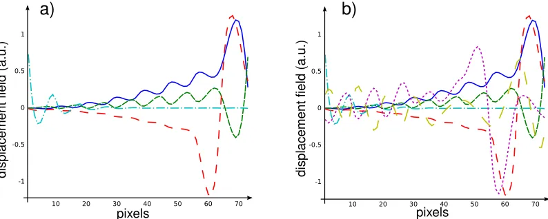
The resulting displacement field (see Fig.1a) is described by 18 degrees of freedom. This displace-ment field basis is used as the micro-scale displacedisplace-ment fields basis (see Fig.1b) and is then used to examplify the above defined procedure. The first macro displacement fields basis is obtained using 4 dofs. Two test displacement fields are therefore used, namelyU⋆
m =Ucm andU⋆m =V18 whereV18is
the last column ofV, that is the dominant mode of the covariance matrix.
Fig. 2a shows the obtained displacement fields basis for 4 macro degrees of freedom. These macro degrees of freedom are those to be used when writing the equilibrium gap matrix at the macro scale, thus limitimg the effect of the measurement noise. Considering two additional macro dofs, the dis-placement fields basis shown on Fig. 2b is obtained by addingU⋆
m =V17. It can be shown this second,
Fig. 2.a) Macro-scale displacement field basis obtained using a single macro element b) Macro-scale displace-ment field basis obtained using 2 macro eledisplace-ments.
4 Conclusion
A two-scales approach for the equilibrium gap method is presented. The projection conditions to be satisfied by the macro displacement field basis have been derived, and a procedure to build the projection operator is proposed. Various strategies can then be drawn in order to get the more robust identification procedure.
References
1. Bornert M., Doumalin P., Dupr´e J.-C., Fazzini M., Gr´ediac M., Hild F., Mistou S., Molimard J., Orteu J.-J., Robert L., Surrel Y., Vacher P. and Wattrisse B., Experimental Mechanics49, (2009) 353-370.
2. Avril S., Bonnet M., Bretelle A.-S., Gr´ediac M., Hild F., Ienny P., Latourte F., Lemosse D., Pagano S., Pagnaco E., Pierron F., Experimental Mechanics48, (2008) 381-402.
3. Amiot F., Hild F., Roger J.P., Int. J. SolidsStruct.44, (2006) 2863-2887. 4. Grediac M., C. R. Acad Sci. Paris309[Serie II], (1989) 1-5.