VISCOUS INCOMPRESSIBLE FLOW SIMULATION USING PENALTY
FINITE ELEMENT METHOD
R.L. SHARMA*
Abstract
:
Numerical analysis of Navier–Stokes equations in velocity– pressure variables with traction boundary conditions for isothermal incompressible flow is presented. Specific to this study is formulation of boundary conditions on synthetic boundary characterized by traction due to friction and surface tension. The traction and open boundary conditions have been investigated in detail. Navier-Stokes equations are discretized in time using Crank-Nicolson scheme and in space using Galerkin finite element method. Pressure being unknown and is decoupled from the computations. It is determined as post processing of the velocity field. The justification to simulate this class of flow problems is presented through benchmark tests - classical lid-driven cavity flow-widely used by numerous authors due to its simple geometry and complicated flow behavior and squeezed flow between two parallel plates amenable to analytical solution. Results are presented for very low to high Reynolds numbers and compared with the benchmark results.Key Words: Viscous incompressible flow; Finite elements, Penalty method, Boundary conditions; Surface traction.
1. Introduction
Major problem in the numerical simulation of incompressible flow is the coupling of the velocity and pressure fields and the correct implementation of pressure boundary conditions. Formulation of boundary conditions is an important stage in solving problems of hydrodynamics and their accuracy largely determines the flow characteristics. Although, form a theoretical point of view, it may be clear what kind of boundary conditions must be prescribed. The solution convergence rate is seriously affected if the coupling among the governing equations is not proper either in the interior or at the boundaries. Different approaches have been used to solve the viscous incompressible flow problems by finite element method [1- 4] usually categorized as mixed formulation (velocity-pressure integrated), segregated and the penalty methods. The accuracy of the various alternatives has been studied extensively in the literature [5]. However, the mixed method is the most intuitive and is based upon simultaneously analysis of momentum and continuity equations treating both the velocity and pressure as unknown. This apparently straightforward way of dealing with the governing equations often leads to consistency problems. The mixed finite element formulation entails large dimensioned system of equations requiring large memory space.
---x Professor, Dept. of Civil Engg., National Institute of Technology, Hamirpur (H.P), India.
e-mail: [email protected]
The stiffness matrix is found to be radically different to the narrow-band type matrix, which is preferred for direct solution. However, these shortcomings are not present in the so called segregated methods.
Another popular strategy to overcome the coupling difficulty is to relax the incompressibility constraint in an appropriate way, resulting in a class of methods with a pseudo-compressibility constraint. Penalty, artificial compressibility, pressure stabilization and projection are some of the methods which belong to this category. In this paper, penalty finite element method which seeks to eliminate the continuity equation to get rid of pressure - the most unusual quantity in the N-S equations has been considered. It is subsequently determined from the velocity at time t without any time lag.
The accuracy of the solution, however, involves specification of the proper boundary conditions [6-8]. Using penalty method neither the pressure nor its normal gradient on the boundaries are known until the velocity field is determined. Prescription of any erroneous boundary stresses may result in distortion of solution in the interior of the domain. Peyret and Taylor [9], in their book on computational fluid mechanics, also identify the specification of correct pressure boundary conditions as the primary difficulty.
In this paper we consider the time-dependent Navier–Stokes equations with traction boundary conditions prescribed on parts of the boundary. The pressure boundary conditions have been replaced by gradient of velocity conditions to avoid distortion of solution. Fully discrete approximation procedure for the solution of transient Navier-Stokes equations based on Crank Noclson scheme in time and finite element method in space is used. It is then applied to classical lid-driven square cavity flow and squeezing flow between parallel plates. The results are compared with benchmark results published in the literature. The comparison shows a good agreement with the model results.
2. Governing Equations
The governing equations for isothermal, viscous incompressible flow over a domain
:
enclosed by the boundary
w
:
*
1
*
2 are:
:
w
w
in
f
p
t
X
X
X
X
2Re
1
.
(1)
div
X
0
in
:
(2)where u is the dependent velocity vector, p is the kinematic pressure, Re is Reynolds number which is reciprocal of the kinematic viscosity
Q
and f is body force vector. The effect of stresses in Eq. (1) is represented by
p
and
2u
/
Re
terms, which are gradients of surface forces, analogous to stresses in solids. The term
p
is pressure gradient and arises from normal stresses that turn up in almost all situations and
2u
/
Re
conventionally represents the shear effect for incompressible flow.3. Boundary Conditions
For conciseness, we breakup
w
:
into two subsets:*
1 and*
2, over which displacements and stresses, respectively are specified. Two transitional relations must be satisfied for fluid at the material boundary i.e. continuity of intensity across the surface and the continuity of normal component of flux vector. For viscous incompressible flow, momentum is the transportable quantity across the interface; hence, specifications of boundary conditions at a surface involve continuity of velocity and continuity of stress.3.1 Continuity of Velocity
On solid walls
w
:
*
1, the velocity must satisfy both no-slip and no-flux conditions. No slip condition requires that the tangential component of the fluid velocity be the same as the tangential component of the velocity of the surface i.e.
X
W
X
W
(3)where,
X
is a given function describing the velocity of the boundary*
1 and t is a unit vector tangent to the boundary. This condition is used almost universally in modeling of viscousflows and is essentially a conservation of tangential velocity; if the boundary isstationary,
X
W
0
and by equation (3) above we have,X
W
0
givingu
v
0
. Similarly, no-flux condition requires that the normal component of the velocity of the fluid must be same as the normal component of the velocity of the boundary i.e.
X
Q
X
Q
(4) where, n is a unit vector that has a direction normal to the boundary. If this were not being the case, the resulting discontinuity would essentially be a rupture or shock in the medium and we have not assumed any event that would cause such a phenomena. Further, any discontinuity across a boundary would result either in a transport of the differences of fluid across the boundary, which would not then be impermeable, or there would be an unbounded positive or negative accumulation of fluid by the wall. Boundary condition (4) is known as no flux or no penetration condition. Combining Eq. (3) and (4) we have
X
g
1on
*
1 (5) The boundary conditions (5) imply that the fluid velocity must match the velocity of the rigid boundary at every point on it. It represents essential or Dirichlet boundary conditions which assign values to dependant variables. It is obtained from kinematic considerations - a condition which relates the motion of the boundary to the fluid velocities and is applicable on rigid and symmetry planes of the boundary*
1.3.2 Continuity of Stress
Boundary tractions and contact forces (because of friction and surface tension) acting on 2 lead to pressure or stress boundary conditions. Considering a small area dA
bounded by a closed contour C and characterized by surface traction tn and surface
S
I
on the element dA is given by
³
³
C Ss WQdA Jdl
I (6)
where,
7
7
is Cauchy stress tensor. The elements of7
7
are associated with normal and tangential forces and can be expressed as the sum of mean hydrostatic stress tensor, pI which tends to change the volume of the fluid element; and deviatoric stress as
7
p
,
Q
X
X
X
T (8) where I is the identity tensor. The partp
,,
represents the stresses due to compression of the fluid. The partQ
X
X
X
T represents viscous stress tensor which tends to distort the body and depend on the velocity of the fluid. It gives the force in a direction parallel to the surface. Substituting the expression for stress tensor in (7) and integrating, we have
³
³
^
`
S
T
S
t
ndA
p
,
Q
u
u
.
Q
dA
(9)Also form Stokes theorem, we have
dl
>
.
@
dA
S
s s
C
³
³
J
J
Q
Q
J
(10)where,
s
Q
.
is the component of gradient operator in the local plane of the
interface.
s.
Q
Q
is the mean curvature of the interface which is expressed as the sum of two radii of curvature R1 and R2 of the interface in any two orthogonal planes. On the right hand side (Eq. 10),J
Q
s.
Q
Q
is the normal curvature force per unit area andJ
s
is the tangential stress associated with gradient of surface tension, both of which will vanish, if either the curvature of the interface or the surface tension vanishes. Using equations (9 -10), the surface force fs become
f
^
p
`
.
dA
>
.
.
@
dA
S
s s
S
T
s
³
,
Q
X
X
Q
³
J
Q
Q
J
(11)Since dA is arbitrary, the integrand must vanish identically giving
˰
p
.
Q
Q
X
X
7.
Q
J
Q
s.
Q
sJ
on
*
2 (12) where ı is the total stress vector acting on a plane perpendicular to the coordinate axis having the unit normal n. It serves as a traction boundary condition at the free surface, typically complementing the Navier-Stokes equations at the far field. The stress vector ı may not necessarily be perpendicular to the plane, i.e. parallel to n, and can be resolved into scalar components i.e. normal and tangential (shear traction).3.3 Normal Stress
The normal stress component, ın of any stress vector in terms of the component of the
stress tensor is the dot product of the stress vector and the unit vector n normal to the surface, thus
˰
n˰
.
Q
Q
(13) Using equation (12), we have
˰
Q>
p
.
Q
Q
X
X
T.
Q
J
Q
s.
Q
SJ
@
.
Q
p
Q
X
X
TQ
Q
J
S.
Q
Q
Q
SJ
.
Q
Q
Q
Q
X
.
.
.
p
Q
J
S
SJ
since
X
X
X
T (14)Noting that
SJ
.
Q
Q
since
SJ
is tangent to the surface, the normal boundary condition (14) can be written as
S
Q
u
.
Q
J
S.
Q
Q
g
2 2 (15)This condition indicates that the interface curvature times the surface tension and pressure must balance the given normal stress. In the case where
*
2 is a planer surface,,
0
.
sQ
Q
the equation (15) reduces to
3.4 Tangential Stress
The tangential stress component, ıtof any stress vector ı in terms of the component of
the stress tensor is given by
˰
t˰
.
WW
(17)where, t is a unit tangential vector. Using (12), we have
˰
W>
Q
Q
Q
X
X
TJ
Q
sQ
S
J
@
W
p
p
Q
W
Q
X
X
TQ
W
J
SQ
Q
W
SJ
W
sJ
in
*
2(18) which indicates that the tangential stress at a surface must be balanced by the gradient of local surface tension. The effect of surface tension applies only in the normal direction since the attractive forces on the molecules between the two mediums will always apply in the direction normal to the fluid interface. Since no such difference in potential forces exists in the tangential direction, equation (18) reduces to
˰
W0
on
*
2 (19)In fact, for incompressible flows, no boundary conditions for pressure are necessary. It is closely related to continuity equation and when the continuity equation is dropped or eliminated, the pressure term will also disappear as is shown later.
In case of time dependant problems, the fluid is also assumed to satisfy the initial condition
X
t 0X
0in
:
(20)velocity field must be solenoidal, i.e.
.
X
00
. A typical divergence free condition correspond to a stationary flow is u0 = 0. For pressure, no initial conditions need to be specified as no time derivatives of pressure appear in the governing equations. Thus we have the boundary conditions
X
g
1on
*
1, (21)S
Q
u
.
Q
g
2;
˰
W0
on 2 and (22)
X
t 0X
0in
:
(23)which together with governing equations (1-2) completely specify the problem.
4. Mathematical Formulation
In penalty function formulation [5], the constrained problem is reformulated as unconstrained one by eliminating the pressure from the equation (1). The idea is to add small term containing pressure to the divergence equation. The obvious choice is
H
P
div
X
0
(24) giving,P
div
X
H
1
(25)where, -independent positive parameter of the order of
10
710
8in double precision calculations. It is believed that the added term introduces damping to the continuity equation and hence reduces the divergence. Using (25), the pressure gradient term can be eliminated from equation (1) to yield:
div
f
Re
1
.
t
2
w
w
X
X
X
X
O
X
(26)parameter, to the momentum balance equation. Strict compliance of incompressibility constraint (Eq. 2) is abandoned in view introduction of penalized term in the momentum equation; thus eliminating the issue of a pressure boundary condition associated with the original primitive variable formulation.
The standard weak form is obtained by the application of weighted residual method i.e. by decretizing the equation (26), multiplying it by an arbitrary test function w which is zero on the boundary and integrating, we have
O
:
:
:
:
Re
.
w
d
w
d
1
.
t
2³
³
»
¼
º
«
¬
ª
w
w
I
X
X
X
X
X
(27)Integrating equation (27) and using the relations
w
2X
div
w
X
w
.
X
,
X
X
w
w
w
w
.
x
.
w
X
together with Gauss divergence theorem
³
³
*
:
div
D
d
:
D
.
Q
d
*
,
with n as outwardnormal and choosing, a=
w
X
,
we obtain the weak formO
:
:
Re
w
.
w
.
d
1
)
.
(
w
w
t
³
»
¼
º
«
¬
ª
w
w
X
X
X
X
X
³
³
³
::
*w
d
*
O
*w
.
d
*
Re
1
d
w
f
X
Q
X
Q
(28)Once the elementary matrices are evaluated and assembled, the Eq. (28) can be expressed as
> @
M
>
K
K
@
^ `
^ `
F
¿
¾
½
¯
®
X
. OX
(29)where, M is the standard mass matrix, K is viscosity matrix arising from viscous terms and
K
Ois so called penalty matrix having the same structure as K. The term F represent aggregate force produced by body forces and stresses (normal and tangential) acting on the surface. It may be observed that matrices K andK
Oare proportional toQ
andO
respectively. In order to impose compressibility constraint, the parameterO
must be selected sufficiently large so that it plays a significant role to yield correct results. If it is too small, compressibility and pressure errors will result and if too large it may result in numerical ill conditioning.Crank-Nicolson scheme [7], with step size % # $&
5. Numerical Examples
5.1 Flow in a Square Cavity
The first benchmark problem attempted using the proposed method is the classical lid-driven cavity flow shown in Figure 1. It has been, widely used by numerous authors viz. Ghia et al. [10], Burgraff [11], Young and Lin [12], Botella and Peyret [13], Eldho and Young [14], etc. Accurate solutions are available in the literature for this problem. The flow in the cavity is driven by shear with upper wall moving from left to right and is characterized by single parameter i.e. Reynolds numb'#&*+ are stationary. The boundary conditions for this problem are Dirichlet type given by
X
X
g
1 and are shown in Figure 1 for each boundary.Figure 1: Configuration of Square Cavity
We solve NS equations (1-2) for a wide range of Reynolds numbers by penalty finite element method for this problem to obtain steady state velocity and pressure fields with initial solution
X
0
.
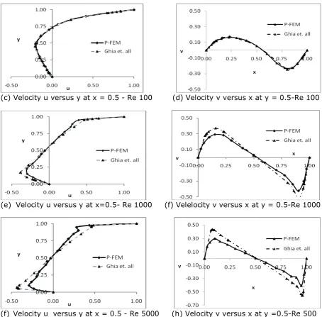
Results have been presented for Re = 10, 100, 1000 and 5000 respectively.For this benchmark problem, the commonly used parameters for comparison of results are the velocity components along the vertical and horizontal lines through the center of the cavity. These results have been plotted for different Reynolds numbers in Figure 2. At Re = 10, the flow is symmetric with respect to the centerline with visible corner eddies. As Reynolds number increases, the center of the main vortex moves toward right downstream corner before it returns toward the center at higher Reynolds numbers. The velocity distribution also provides a good measure of the effect of viscosity. The trend from rounded profile at low Reynolds number to the flattened profile at high Reynolds number is clear. The symmetric pattern up to Re = 100 is due to the vanishing of the convective terms in Equation 1. As the Reynolds number increases (inviscid flow), the flow becomes unsymmetrical with the dominance of inertia terms.
(c) Velocity u versus y at x = 0.5 - Re 100 (d) Velocity v versus x at y = 0.5-Re 100
(e) Velocity u versus y at x=0.5- Re 1000 (f) Velelocity v versus x at y = 0.5-Re 1000
(f) Velocity u versus y at x = 0.5 - Re 5000 (h) Velocity v versus x at y =0.5-Re 500
Figure 2: Velocity profiles along central horizontal and vertical line of the cavity For accuracy, the computed results are compared with benchmark solutions and are shown in Figure 2 for Re = 10, 100, 1000 and 5000. The comparison show a close agreement between the computed and benchmark results.
These figures also indicate that stable solutions are obtained for Reynolds numbers as high as 5000. However, it has been noticed that as the Reynolds number increases, the convergence becomes slow owing to the diminishing thickness of the viscous layer, thus increasing the number of iterations required to attain the same degree of accuracy. This behavior can be noticed from Table 1 where characteristic results for velocity are given along the vertical line through the center of the cavity. The minimum of u along the center of the vertical line at x = 0.5 is denoted by umin. Similarly maximum and minimum
of v along the horizontal line at y = 0.5 are denoted by vmax and vmin respectively. The
Table 1: Characteristic values of the solution extrema on the horizontal and vertical line through center of the cavity.
Re P-FEM Solution Ref. (20) Solution
umin vmax vmin J umin vmax vmin J
10 -0.1950 0.1736 -.01803 186 - - -
-100 -0.1921 0.1647 -0.2243 213 -0.2058 0.1750 -0.2453
-1000 -0.2973 0.2910 -0.4240 839 -0.3828 0.3709 -0.5155
-5000 -0.2912 0.2991 -0.4066 7500 -0.4364 0.4364 -0.5540
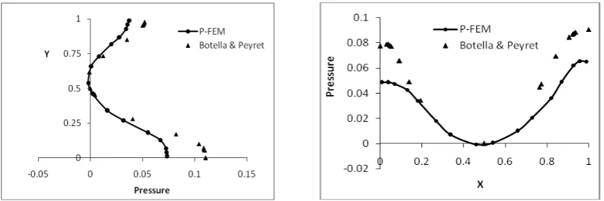
-The pressure was computed once the velocity profile was obtained. -The pressure variation along the horizontal and vertical lines through the cavity center is shown in figure 3 for Re = 100, 1000 and 5000.
Figure 3: Pressure profiles along central vertical and horizontal lines of the cavity
The comparison of pressure variation is also made with the model results of Botella and Peyret [13] for Re = 1000, wherein, the results of pressure field are given after setting the pressure equal to zero at the center (0.5, 0.5) of the cavity. Therefore, for the sake of comparison, free scale factor is chosen to make the pressure zero at the center of the cavity. The comparison is shown in figure 4 for Re = 1000. The agreement is seen to be good with the model results. However, small difference near the two ends is caused by effect of element division in the present case.
Figure 4: Comparison of pressure profiles along central vertical and horizontal lines of the cavity
5.2 Squeezing flow between parallel plates
two-dimensional; the central axis of the channel is taken as the x-axis and the y-axis perpendicular to it. It is also assumed that the plates move symmetrically with respect to the central axis of the channel. The dimensions of the modelling region are shown in Figure 5. The movement of plates would impart momentum to the fluid and would set up a velocity gradient in the fluid. Assuming a strong fluid-wall interaction, we expect robust momentum transfer and Dirichlet boundary conditions at the walls and traction boundary conditions at the outflow as follows:
0
0
0
0
0w
w
y
at
y
u
and
v
B
y
at
v
v
and
u
(30)
The plates are considered long enough so that the flow at the exit planes is fully developed and the velocity profile become invariant. The boundary conditions at these planes follow from equation 23 and are:
Figure 5: Dimensions of the Modeling Region and Boundary Conditions
at
x
L
x
u
u
r
w
w
.
Q
0
(31)Since the problem is transient in nature and has to be solved with appropriate initial conditions which are assumed as
:
in
0
t
at
0
X
(32)The analysis has been carried out with
U
Q
0
. The results are shown in Figures 6 and 7.
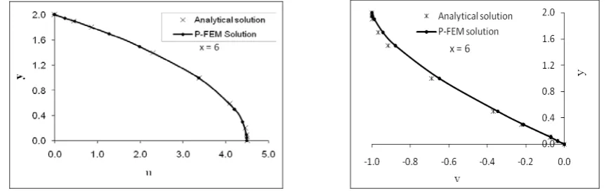
Figure 6: Comparison of computed velocity profiles with analytical solution
Figures 6a shows the variation of velocity u with y at x = 6. It shows that the velocity u varies parabolically. Figure 6b shows the variation of velocity component v with y. Clearly the velocity v varies from -1.0 at the boundary to zero at the center as anticipated. Figures 6a and 6b also show the comparison of computed velocity profiles with the approximate analytical solution of Nadai [15]. It can be observed that there is an
The pressure has been calculated by post-processing the velocity field using
.
)
u
.
(
P
O
The variation of pressure along the length of plate has been plotted at0
y
y
rr
, where y0 is the y -coordinate of the Gauss point. Figure 7a shows the plot ofpressure variation at
y
rr
0
.
02
along the length of the plate, whereas, figure 7b shows the pressure variation across the gap between the plates atx
rr
0
.
02
. The pressure at the walls is marginally higher than that in the central core. These figures indicate that in this case bothw
3
/
w
x
asw
3
/
w
y
are non-zero.
Figure 7: Comparison of computed pressure profiles with analytical solution
6. Conclusion
We present the successful application of penalty finite element method to viscous incompressible flow problems governed by Navier-Stokes equations. The penalty variational formulation using finite element approximation has been constructed and discussed. The solution requires additional boundary conditions about the velocity field and its velocity gradients at the natural boundaries of the flow domain. Formulation of boundary conditions on synthetic boundary characterized by traction due to friction and surface tension has been formulated and discussed in detail.
The solutions presented for the two standard problems are representative of the most accurate solutions obtained for each case. With good agreement between the computed results and benchmark solutions it is concluded that penalty finite element method is a convenient way to satisfy the incompressibility constraint and to eliminate the pressure as an unknown from the formulation, thus reducing the number of degrees of freedom in the discretization. It can be successfully applied to solve incompressible viscous as well as inviscid fluid problems over a wide range of Reynolds numbers.
References
[1] Carry J.F. and Krishnan R., Penalty Finite Element Method for Navier – Stokes Equations, Journal of Computer Methods in Applied Mechanics and Engineering, 42, 1983, pp 183–224.
[2] Hughes T.J.R., Liu W.K. and Brooks A., Finite Element Analysis of Incompressible Viscous Flow by the Penalty Function Formulation, Journal of Computational Physics, 30, 1979, pp. 1-60.
[4] Jobelin M., Lapuerta C., Latche J.C., Angot Ph. and Piar B., A finite element penalty–projection method for incompressible flows, Journal of Computational Physics, 217, 2006, pp 502-508.
[5] Gresho P. M. and Sani R. L., On the Pressure Boundary Conditions for the Incompressible Navier – Stokes Equations, Int. Journal for Numerical Methods in Fluids, 7, 1987, pp 1111-1145.
[6] Liu J., Open and Traction Boundary Conditions for the Incompressible Navier-Stokes Equations, Journal of Computational Physics, 228, 2009, pp 7250-7267.
[7] Barth W.L. and Carey G.F., On a Boundary Condition for Pressure-Driven Laminar Flow of Incompressible Fluids, Int. Journal of Numerical Methods in Fluids, 54, 2007, pp 1313–1325.
[8] Dai X., Finite Element Approximations of the Pure Neumann Problem using Iterative Penalty Method, Journal of Applied Mathematics, 186, 2007, pp 1367-73.
[9] Peyret R. and Taylor T.D., Computational Method for Fluid Flow, Springer-Verlog Berlin, 1983.
[10] Ghia U., Ghia K.N. and Shin C.T., High-Re Solutions for Incompressible Flow Using the Navier-Stokes Equations and a Multigrid Method, Journal of Computational Physics, 48, 1982, 387-411.
[11] Burggraf O.R., Analytical and Numerical Studies of the Structure of Steady Separated Flows, Journal of Fluid Mechanics, Part 1, 1966, pp 113-151.
[12] Young D.L. and Lin Q.H., Application of Finite Element Method to 2-D Flows, Proc. 3rd National Conference in Hydraulic Engineering, Taipei, 223-242.
[13] Botella O. and Peyret R., Benchmark Spectral Results on the Lid-Driven Cavity Flow, Comp. & Fluids, 27, 1998, 421-433.
[14] Eldho T.L. and Young D.L., Two Dimensional Incompressible Viscous Flow Simulation Using Velocity-Vorticity Duel Reciprocity Boundary Element Method, Journal of Mechanics, Vol. 20, 2004, pp 177-185.