DEVELOPMENT OF OPTIMIZATION ALGORITHMS FOR
UNCERTAIN NONINEAR DYNAMICAL SYSTEM
(PEMBANGUNAN ALGORITMA PENGOPTIMUMAN UNTUK
SYSTEM TAK LINEAR TAK PASTI)
MOHD ISMAIL BIN ABD AZIZ ROHANIN BINTI AHMAD
RESEARCH VOT NO: 71910
Jabatan Matematik Fakulti Sains
Universiti Teknologi Malaysia
ACKNOWLEDGEMENT
DEVELOPMENT OF OPTIMIZATION ALGORITHMS FOR UNCERTAIN NONINEAR DYNAMICAL SYSTEM
(Keywords:Optimal Control,nonlinear, model reality,DISOPE, momentum terms)
Nonlinear optimal control problems are problems involving real world situations where the objectives are the maximization of the return from, or the minimization of the cost of, the operation of physical, social, and economic processes. Algorithms used to solve these problems are expected to satisfy the objectives consistently and since time translates into cost, must also be fast. An algorithm that definitely can satisfy the objectives is the Dynamic Integrated Systems Optimization and Parameter Estimation (DISOPE) algorithm. However, this algorithm has an inherent problem of slow convergence due to its gradient descent type updating mechanism. Hence, the purpose of this study is to overcome this convergence problem by modifying the mechanism. Two approaches were chosen for this purpose. The first is the use of momentum terms and the second is the parallel tangent method. Two new algorithms named DISOPE-MOMENTUM and DISOPE-PARTAN sprouted from these modifications and extensive simulations were performed to observe their performances. To strengthen the findings, theoretical analyses were done on each algorithm. These include optimality, stability, convergence, and the rate of convergence analyses. Based on the results of these simulations, we compared the number of iterations needed by each algorithm to arrive at the optimal solution and the CPU time taken for each algorithm to execute the search. From the theoretical analyses, comparisons were done on the speeds of contraction of the algorithms. Both new algorithms managed to arrive at the optimum in fewer numbers of iterations and in shorter CPU times than DISOPE without compromising on the accuracy of the solutions. The new algorithms also boast faster contractions. Both new algorithms performed better than DISOPE. This study succeeded in overcoming the problem of slow convergence and with the modifications, the new algorithms become more efficient in solving the optimal control problems.
Key researchers:
Asc. Prof. Dr. Mohd Ismail Abd Aziz Rohanin Ahmad
Email: [email protected]
Tel. No: 07-5534231 / 019-7538204
ABSTRAK
Masalah kawalan optimum tak linear adalah masalah dunia nyata yang berobjektifkan pemaksimuman hasil, atau peminimuman kos operasi fizikal, proses-proses sosial atau ekonomi. Algoritma yang ingin digunakan untuk menyelesaikan masalah-masalah ini harus berupaya memenuhi objektif tersebut, dan disebabkan masa boleh ditafsir sebagai kos algoritma ini juga harus pantas. Sebuah algoritma yang berupaya memenuhi objektif di atas ialah algoritma Pengoptimuman Sistem Bersepadu Dinamik dan Penganggaran Parameter. Walau bagaimanapun, algoritma ini mempunyai masalah penumpuan lamban yang diwarisi daripada mekanisme pengemaskiniannya yang tergolong ke jenis penurunan gradien. Tujuan kajian ini ialah mengatasi masalah penumpuan di atas dengan cara mengubahsuai mekanisme tersebut. Dua pendekatan telah dipilih untuk tujuan ini. Yang pertama
menggunakan sebutan momentum dan yang kedua menggunakan kaedah tangen selari. Dua algoritma baru yang dinamakan MOMENTUM dan DISOPE-PARTAN terhasil daripada ubahsuaian ini dan simulasi secara ekstensif telah dijalankan untuk meninjau prestasi masing-masing. Untuk memampankan hasil penemuan, analisis secara teori telah dilakukan untuk setiap algoritma. Analisis-analisis ini termasuk Analisis-analisis keoptimuman, kestabilan, penumpuan dan Analisis-analisis kadar penumpuan. Berdasarkan hasil simulasi, kami bandingkan bilangan lelaran yang diperlukan oleh setiap algoritma untuk mencapai penyelesaian optimum dan juga masa CPU yang diambil oleh setiap algorithma untuk melaksanakan carian. Daripada analisis secara teori, perbandingan telah dibuat terhadap kecekapan, kerumitan dan kepantasan pengecutan algoritma. Kedua-dua algoritma baru ini berupaya mencapai optimum masing-masing dengan bilangan lelaran dan masa CPU kurang daripada DISOPE, tanpa menjejas kejituan penyelesaian. Pengecutan
algoritma-algoritma ini juga lebih pantas. Kedua-dua algoritma baru ini
TABLE OF CONTENTS
CHAPTER TITLE PAGE
TITLE PAGE i
DECLARATION ii
ACKNOWLEDGEMENTS iii
ABSTRACT iv
ABSTRAK v
TABLE OF CONTENTS vi
LIST OF TABLES xi
LIST OF FIGURES xii
1 INTRODUCTION 1
1.0 The Continuous Optimal Control Problem 1 1.1 Methods for Solving the Continuous Optimal
Control Problem
2
1.2 The Variational Approach to Optimal
Control Law 3
1.2.1 The Necessary Optimality Conditions 4 1.2.2 Difficulties Facing the Nonlinear Optimal
Control Problems
5
1.3 LQR Problem as Model 6
1.4 Model-Reality Differences 9 1.4.1 DISOPE Algorithm 9 1.4.2 Problems Faced by Gradient Descent
Methods 10
1.5 Statement of Problem 12
1.6 Research Objectives 12
1.7 Scope of Research 12
1.8 Contributions of the Research 13 1.8.1 Contributions to Algorithm Development 14 1.8.2 Contribution to Theoretical Analysis 14 1.8.3 Contribution to Software Implementation and Algorithm Testing 15 1.8.4 Contribution to the Field of Gradient Descent
Algorithm 15
1.9 Outline of Thesis 16
1.10 Summary and Conclusion 17
2 LITERATURE REVIEW 18
2.1 Introduction 18
2.2 Other Approaches in Solving Optimal Control
Problems 19
2.3 Background of DISOPE Algorithm 21
2.4 Gradient Descent Algorithm 23
2.5 Back Propagation Algorithm 27
2.5.1 A Perceptron 27
2.5.2 Multilayer Perceptron 29 2.5.3 Representation of the Back Propagation
Algorithm 30
2.5.4 Approaches to Overcome the Slow
Convergence 30
2.6 Momentum Term 35
2.7 Parallel Tangent 37
2.8.1 Link to 2-D Systems 41 2.8.2 Abstract Model of Multipass Processes 42
2.8.3 An Abstract Model of the Linear Multipass Process of Constant Pass Length in the
Form of a Unit Memory Repetitive Process 44 2.8.4 Properties of the Linear Unit Memory
Repetitive Processes 44 2.8.5 DISOPE as 2-D System 46
2.9 Summary and Conclusion 47
3 DISOPE ALGORITHM 49
3.1 Introduction 49
3.2 Problem Formulation 49
3.3 DISOPE Algorithm 55
3.4 DISOPE with LQR as Model 55
3.5 The Algorithm Mapping of DISOPE 58
3.6 The Optimality Analysis 63
3.6.1 A Unit Memory Repetitive Process
Interpretation 64
3.6.2 DISOPE as Linear Multipass Process 66 3.6.3 The Optimal Condition of ROP and Its Linear Unit Memory Repetitive Process Form 69 3.7 The Stability and Convergence Analyses of DISOPE 72 3.7.1 The Stability Analysis 72 3.7.2 The Convergence Analysis 74
3.8 Numerical Examples 76
3.9 Summary and Conclusion 85
4 FURTHER ANALYSES OF DISOPE 86
4.1 Introduction 86
4.3 Map C as a Gradient Descent Algorithm 88 4.3.1 Generating the Error Function 89 4.4 DISOPE and the Basic Characteristics of the Gradient
Descent Method 91
4.4.1 Numerical Examples 92 4.5 The Analysis of the Rate of Convergence 95 4.5.1 Establishing the Existence and Uniqueness of y) in DISOPE 96 4.5.2 Establishing the Convergence Rate 98
4.6 Summary and Conclusion 101
5 DISOPE-MOMENTUM ALGORITHM 103
5.1 Introduction 103
5.2 Modification of Map C 104
5.2.1 Similarities Between Map C and BP
Algorithm 104
5.2.2 The Inclusion of the Momentum Term 105 5.3 The Effects of the Momentum Term on DISOPE 107 5.3.1 Numerical Examples 108
5.4 DISOPE-MOMENTUM Algorithm 115
5.6 Summary and Conclusion 118
6 DISOPE-PARTAN ALGORITHM 119
6.1 Introduction 119
6.2 Modification of Map C 119
6.2.1 The Gradient-PARTAN Method 120 6.2.2 The Incorporation of PARTAN to Map C 122 6.3 The Effects of Gradient-PARTAN 124 6.3.1 Numerical Examples 125
6.4 DISOPE-PARTAN Algorithm 132
9 CONCLUSION 136
9.1 Introduction 136
9.2 Summary of significant Findings 136
9.3 Further Research 140
LIST OF TABLES
TABLE NO. TITLE PAGE
3.1 The result of the algorithm’s performance with different values of the relaxation gains and convexification
factors 78
3.2 The algorithm’s performance for Example 3.2 81
3.3 The simulation results of Example 3.3 83
4.1 Results of simulation with different values of Q 93 4.2 Results of simulation with different values of R 94 5.1 Algorithm’s performance of Example 5.1 with the
addition of momentum terms 108
5.2 The comparison of the performance of DISOPE and
DISOPE-MOMENTUM foe Example 5.2 112
6.1 The algorithm’s performance of Example 6.1 with the
incorporation of PARTAN step 126
6.2 Comparisons of the final performance of DISOPE and
LIST OF FIGURES
FIGURE NO. TITLE PAGE
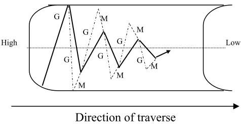
2.1 The different terrains of the surface of a nonlinear
function 24
2.2 The oscillation phenomenon 25
2.3 The zigzagging phenomenon 25
2.4 The schematics of the problems faced by gradient
descent algorithms 27
2.5 A single layer perceptron 28
2.6 A simple three-layer perceptron 29
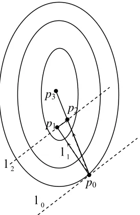
2.7 The locus of weights with the momentum terms 36 2.8 Locus for the search for a quadratic function 38 2.9 The points of tangency of the two parallel lines define
a line that parallels the ravine 39
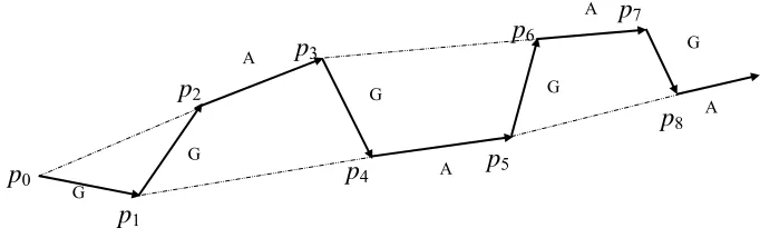
2.10 The path taken by the gradient-PARTAN. 40
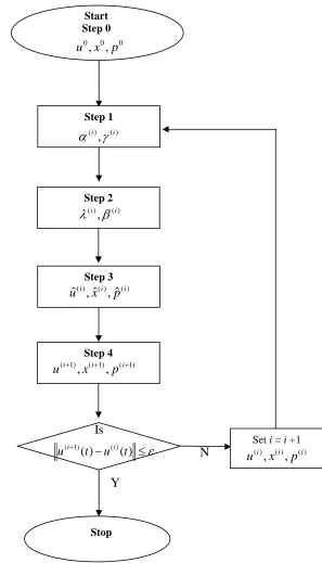
3.1 The flow chart of DISOPE algorithm 56
3.2 The final responses of DISOPE for Example 3.1 (vii) 79 3.3 The final responses of DISOPE for Example 3.2 (iv) 82 3.4 The final responses of DISOPE for Example 3.3 (iii) 84
4.1 Composite map of DISOPE 88
4.2 Comparisons of closeness between two different initial solutions and the optimal solution (a) Result for Q =
2I2; (b) Result for Q = [22.40 4.480; 4.480 0.896] 93
5.1 The effects of the momentum terms on the search
direction 106
5.2 The comparison of the performance indices of
Example 5.1 110 5.3 The comparison of the control variation norms of
DISOPE and DISOPE-MOMENTUM for Case (i) of
Example 5.1 111
5.4 The comparison of the performance indices of (a) DISOPE and; (b) DISOPE-MOMENTUM, for Case
(i) of Example 5.2 113
5.5 The comparison of the control variation norms of (a) DISOPE and (b) DISOPE-MOMENTUM, for Case (i)
of Example 5.2 114
5.6 The flow chart of DISOPE-MOMENTUM algorithm 117
6.1 The zigzagging phenomenon 121
6.2 The optimum is reachable along the line through p0
and p2 122
6.3 The vectors involved in the general gradient-PARTAN
search 123
6.4 The comparisons between the performance indices of
(a) DISOPE; (b) DISOPE-PARTAN 127
6.5 The comparisons between the control variation norms
of DISOPE and DISOPE-PARTAN of Example 6.1 128 6.6 The graph showing the final states x(t) of Case (iii)
satisfying the end-point condition of x1(2) = 0 130
6.7 The comparisons of the performance indices of (a)
DISOPE and (b) DISOPE-PARTAN of Case (iii) 131 6.8 Comparisons between the control norms of DISOPE
and DISOPE-PARTAN of Case (iii) 131
LIST OF SYMBOLS AND ABBREVIATIONS
i
a - The input of node i
A - A time-invariant state matrix for the system dynamics of an LQR model
, , , , , mp mp mp
mp mp mp A B C D F J
⎫⎪ ⎬
⎪⎭ - Constant coefficient matrices of the multipass processes 1
i
b+ - The initial conditions, disturbances, and control input effects
B - A time-invariant control matrix for the system dynamics of an LQR model
0
B - As defined in Equation (3.76)
*
A - As defined in Equation 3.22
*
B - As defined in Equation 3.22
C - As defined in Equation 3.46
1
C - As defined in Equation 8.33
N
C - The learning rate
2n m
C + - Bounded mappings
( )
i
d t - Interpass disturbance
D - A set of constraints
1
D - As defined in Equation 3.79
1
M
D - As defined in Equation 7.16
3
D - As defined in Equation 8.32
( )
E w - Error function of a back propagation algorithm ( )
( ) i y
n
E - The Euclidean space
0
E - As defined in Equation 3.83
0
E% - As defined in Equation 3.82 1, 2
E E - Matrices representing the contributions from r r1, 2
Eς - A Banach space
( )
f ⋅ - Plant dynamics of the model
* ( )
f ⋅ - Plant dynamics of the real process ( ), ( )
f n g n - Complexity functions, with n input size ( )
F λ - As defined in Equation 3.97
( )
P
F λ - As defined in Equation 8.31
1( ), 2( )
g ⋅ g ⋅ - Vectors representing the model reality differences G - The gradient descent direction
( )
G t - A m n× Kalman gain matrix
h - Step size
1, 2, 3
h h h - Lipschitz constants 1 , 2 , 3
DM DM DM
h h h - Lipschitz constants for DISOPE-MOMENTUM h - Input size in time complexity analysis
( )
H ⋅ - The Hamiltonian
,
i j - Indices
I - The identity matrix
J - The performance index of the LQR model
J( - As defined in Equation 3.65
*
J - The real cost functional or performance index
J′ - The Lagrangian functional
ea
J - The performance index of the augmented EOP
EOP
J - The performance index of EOP
MOP
J - The performance index of MOP
MMOP
J - The performance index of MMOP
( )
y
K - As defined in Equation 3.41
1, 2
l l - Lines
( )
L ⋅ - Performance index of the model *
( )
L ⋅ - Real performance measure function
Lς - A bounded linear operator of Eς into itself
M - The momentum direction
( ( )), ( ( )) ( ( )), ( ( )) o f n O f n
f n f n
⎫ ⎬
Θ Ω ⎭ - Sets of complexity functions
( )
p t - The costate vector
0, 1,
p p K - Search points
P - PARTAN step direction
* ( )
0
( i ( ), , )f
P y t t t - As defined in Equation 3.52
y
P - A matrix of PARTAN parameters
Q - Symmetric state weighting matrix for the LQR model ( )
r Lς - Spectral radius
1, 2
r r - Scalar modification factors
R - Symmetric control weighting matrix for the LQR model ,
R Q - The augmented weighting matrices ,
S V - Weights for the terminal conditions of the LQR model
ˆ
S - An arbitrary set in the Euclidean space
j
S - The sum of all weighted inputs from node i
,
t τ - Time
0
t - Initial time
,
f
t T - Terminal time
j
t - A set of target outputs
( )
u t - The control vector
o
u - Optimal control
ˆ( ), ( ), ( )ˆ ˆ
( ), ( ), ( )
v t z t P t - Variables used in the updating step *
V - As defined in Equation 3.22
w - A vector of all weights between nodes and i j
y
W - A matrix of momentum parameters
Wς - A linear subspace
( )
x t - The state vector
o
x - Optimal state
0
x - Initial state
j
x - Actual output of a network
( ) ( )
i
y t - The process output
y) - Limit point of the sequence of terms ( )
i
Y t - Pass profile i
,
Y∞ y∞ - The limit profile ( ), ( )t t
α γ - Parameter estimates for the value differences between reality and model
s
β - A search parameter
( ) 1
i
Γ - As defined in Equation 3.23
( ) 2
i
Γ - As defined in Equation 3.23
η - Step size parameter of the gradient descent algorithm 0
( , , )t t tf
η - As defined in Equation 3.52
m
η - Momentum Learning rate of the back propagation
θ - A predetermined threshold value
1, 2, 3
ϑ ϑ ϑ - Contraction coefficients
κ - A constant; κ∈[0, )∞
( ), ( ), ( ), ( )
t t t t
λ β
μ ξ
⎫ ⎬
⎭ - Scalar multipliers
( ), ( )t t
λ β - Augmented scalar multipliers
,
x p
μ μ - As defined in Equation 3.50
, ,
u x p
℘ ℘ ℘ - PARTAN parameters
ς - Pass length
0 ( ,t tf)
σ - As defined in Equation 3.109
( )
φ ⋅ - Final weighting function – scalar valued ( , )t
φ τ - As defined in Equation 3.33
21( , ),t tf 0 2( , )t
φ φ τ - As defined in Equation 3.36
11( , ), ( , )t tf 0 1 t
φ% φ τ% - As defined in Equation 3.37
21 0 21 0
2
( , ), ( , ),
( , )
f f
f
t t t t
t
φ φ
φ τ
⎫⎪ ⎬ ⎪⎭
% %
% - As defined in Equation 3.38
Φ - Symmetric terminal weighting matrix for the LQR model
Φ( - As defined in Equation 3.63
*
Φ - Real terminal measure
χ - Lagrange multiplier
Ψ( - As defined in Equation 3.64
*
Ψ - Real terminal constraint vector *
Ψ - As defined in Equation 3.36
*
Ψ% - As defined in Equation 3.37 , u, x, p
ϖ ϖ ϖ ϖ - Momentum parameters
0 ( , , , )t t tf τ
Ω - As defined in Equation 3.53
, f g
∇ - Gradient of a function
( )
( )⋅ ∞ - Limit profiles
2
⋅ - The Euclidean norm used in the thesis
DISOPE - Dynamic Integrated Systems Optimization and Parameter Estimation
DISOPE-MOMENTUM
- DISOPE with momentum terms
DISOPE-PARTAN - DISOPE with PARTAN step
EOP - Expanded Optimal Control Problem
Estimation
MMOP - Modified Model Based Optimal Control Problem MOP - Model Based Optimal Control Problem
CHAPTER 1
INTRODUCTION
1.0 The Continuous Optimal Control Problem
Suppose that a plant is described by the time-varying dynamical equation *
( ( ), ( ), )
x&= f x t u t t (1.1)
where f*:¡ nס m× →¡ ¡ n representing a set of equations describing the process with ( ) n
x t ∈¡ as the state vector, ( ) m
u t ∈¡ as the control input, and t∈¡ as the time. Let the functional
0
* *
( ( ))f tf ( ( ), ( ), )
t
J =φ x t +
∫
L x t u t t dt (1.2) be the associated cost function or performance index, where [ ,t t0 f] is the time interval. In Eq. (1.2) :φ ¡ n →¡ is a scalar valued function called the finalweighting function, which depends on the final state and final time. The weighting function *
: n m
L ¡ ס × →¡ ¡ is a continuous function, and it depends on the state and input at intermediate times in [ ,t t0 f]. In both Eqs. (1.1) and (1.2), ( )⋅* represents the original problem formulation.
By assuming that the state of the system at initial time is given with value
0 0
( )
0
* *
( )
min ( ( ))f tf ( ( ), ( ), )
t
u t J =φ x t +
∫
L x t u t t dt (1.3)subject to *
( ( ), ( ), )
x&= f x t u t t (1.4)
0 0
( )
x t =x (1.5)
In order to emphasize time as the argument of the functions, they are referred to as either the control trajectory, which means the time path of the control vector, or the state trajectory, which means the time path of the state vector. If time does not enter explicitly as an argument of f*, we say that the system is autonomous.
1.1Methods for Solving the Continuous Optimal Control Problem
Two established methods for accomplishing the minimization are the method of Dynamic Programming developed by Bellman (1957) and the variational
approach of Pontryagin (Pontryagin et al. 1962).
The method of dynamic programming can handle control and state
The variational approach of Pontryagin is called the minimum principle. It generalizes the calculus of variations to include problems where optimization is not achieved by calculus. It is an extension of Weierstrass’ necessary condition to cases where the optimal functions are bounded. It follows directly from the general continuous-time dynamic programming equations.
The minimum principle deals with one extremal at a time. In optimal control terminology, its states that a minimizing path must satisfy the Euler-Lagrange equations where the optimal controls maximize the Hamiltonian within their bounded region at each point along the path (Hocking, 1991). This transforms the calculus of variation problem to a nonlinear problem at each point along the path.
1.2. The Variational Approach to Optimal Control Law
The algorithms discussed in this research used the variational approach in their course toward finding the solutions of the optimal control problems. Thus we steer our discussion in the direction of this approach.
The optimal control problem defined in Eqs. (1.3), (1.4), and (1.5) in Sec.1.1 is a constrained minimization problem. The variational approach for solving this problem is to eliminate the existence of constraints and turn the problem into an unconstrained problem. Adjoining the constraints to the performance index using Lagrange multipliers does this. Thus a new functional called the Lagrangian functional is defined. This approach was introduced by Lagrange (Rao, 1984). According to the Lagrange theory, the minimum of the original problem is achieved by finding the minimum of the new unconstrained functional (Lewis and Syrmos, 1995).
Suppose that ( )p t T∈¡ is the multiplier for the system defined by Eq. (1.4). n Then, the new Lagrangian functional to be minimized can be defined as
0
( ( ), )+ T[ ( ( ), ( ), ) ( ) ( ( ( ), ( ), )T )]
t
where ( )p t is usually referred to as the costate function. From Eq. (1.6), if we define a function termed the Hamiltonian, which is
( ( ), ( ), ( ), )H x t u t p t t =L x t u t t( ( ), ( ), )+p t( )T f x t u t t( ( ), ( ), ), (1.7) then Eq. (1.6) can be rewritten as
0
( ( ), )+ T[ ( ( ), ( ), ( ), ) ( )T ]
t
J′ =φ x T T
∫
H x t u t p t t −p t x dt& (1.8)The problem is now reduced to a problem of finding the minimum of a functional represented by Eq. (1.8). From the calculus of variation, we know that the minima of such functionals happened at points where the gradients have the values of zero. The conditions where the gradients diminished are called the necessary
optimality conditions. Thus to find the solution of this problem, we have to clearly define these conditions.
1.2.1 The Necessary Optimality Conditions
The necessary optimality conditions for solving Eq. (1.8) are derived by setting all the gradients of the Hamiltonian with respect to x u, , and p, respectively, to zero (Lewis and Syrmos, 1995). The criteria are listed below.
( ) 0 or ( )
xH p t p t xH
∇ + & = − & = ∇ (1.9)
0
uH
∇ = (1.10)
( )∇pH−x t& =0 or x t&( )= ∇pH (1.11) Eqs. (1.9), (1.10), and (1.11) are also referred to as the costate equation, stationarity condition, and the state equation respectively. Eqs. (1.9) and (1.10) are also called Euler’s or Euler-Lagrange equations (Lewis and Syrmos, 1995; Bryson, 1996). The solution of the optimal control problem defined by Eqs. (1.3), (1.4), and (1.5) is arrived at by solving Eqs. (1.9), (1.10), and (1.11) together with the following boundary conditions
0 0
( )
x t =x (1.12)
and
( ) ( ( ))
f
f x t t
Even though the manner for finding the solution of the continuous optimal control problem is well outlined, the actual job of finding the solution is by no means effortless. The variational approach to the necessary optimality conditions leads to a nonlinear two-point boundary-value problem (Kirk, 1970) having boundary
conditions specified at two separate points in time (Jacob, 1974) given by Eqs. (1.12) and (1.13).
The optimal control law depends on the solution of the nonlinear two-point boundary-value problem, which in general, are difficult problems to solve (Kirk, 1970; Jacob, 1974; Bryson and Ho, 1975; Lewis and Syrmos, 1995) due to the high degree of nonlinearity involved. Analytical solutions are close to impossible; therefore, numerical solutions are usually sought for. Techniques available for solving the nonlinear two-point boundary-value problem include the steepest descent, variations of extremals, and quasilinearization (Kirk, 1970). All these methods begin with the necessary optimality conditions obtained from the application of the minimum principle of Pontryagin.
1.2.2 Difficulties Facing the Nonlinear Optimal Control Problems
Most optimal control problems are very nonlinear. Without a doubt, a ‘good’ model of the real dynamical process must have high degree of nonlinearity.
However, using a good model representation of the real problem does not translate into ease of solution. Basically, there are at least three foreboding problems with nonlinear optimal control problem as described above. The first one is due to the variational approach itself, which ends up with a nonlinear two-point boundary-value problem as the necessary optimality conditions. As mentioned earlier, these
problems are difficult to solve.
of constraints might define a feasible region that is difficult to find (Shang, 1997). Furthermore, even when the feasible region is located, if both the objective functions and the set of constraints are not convex, the convergence to a global optimum is not guaranteed (Stoer and Witzgall, 1970; Koo, 1977; Cesari, 1983; Bunday, 1984; Rao, 1984; Beale, 1988; Shang, 1997).
Hence, a class of methods tries to do away with the ‘good’ model and instead use ‘easy-to-solve’ models to approximate the original problems. Here is where the Linear-Quadratic-Regulator (LQR) problem comes in handy.
1.3 LQR Problem as Model
To overcome the difficulties mentioned above, we resort to modeling the original problem defined by Eqs. (1.3) - (1.5), which consisted of both nonlinear system dynamics and performance index with ‘simpler’ functions. For this purpose, we use the linear-quadratic regulator (LQR) problem. With LQR as model, the system dynamics are represented as linear differential equations and the performance index is a quadratic function in terms of the state and control variables. In LQR problems, the resulting two-point boundary-value problem is linear and is relatively easy to solve (Becerra, 1994), obtaining a linear optimal control law (Kirk, 1970). In LQR problems it was found that it is possible to obtain the optimal law, by
numerically integrating a matrix differential equation of the Riccati type.
With the LQR as model, the optimal control problems are defined as follows:
0
( )
1 1
min ( ) ( ) ( ) ( ) ( ) ( )
2 2
f
t
T T T
f f t
u t J = x t Φx t +
∫
⎡⎣x t Qx t +u t Ru t dt⎤⎦ (1.14)subject to
( ) ( )
x&= Ax t +Bu t (1.15)
0 0
( )
x t =x (1.16)
the time-invariant matrices of the system dynamics and control distribution respectively. The Hamiltonian function defined in Eq. (1.7) becomes
(
)
(
)
1
( ) ( ) ( ) ( ) ( ) ( ) ( )
2
T T T
H = x t Qx t +u t Ru t +p t Ax t +Bu t (1.17) with the state equation becoming
( ) ( )
x&= Ax t +Bu t (1.18)
and the costate equation ( ) ( ) T ( ) p t Qx t A p t
−& = + (1.19)
The stationarity condition is now
0 ( ) T ( )
Ru t B p t
= + (1.20)
Furthermore, by rearranging Eq. (1.20) we get the basic expression for the control input as
1
( ) T ( )
u t = −R B p t− (1.21)
The boundary conditions become
0 0
( )
x t =x (1.22)
and
( ) ( ( )) ( ) ( )
f
f x t t f f
p t = ∇ φ x t = = Φ t x t (1.23)
1.3.1 Solving the LQR Optimal Control Problem
Kalman showed that the linear quadratic optimal control problem could be solved numerically in an elegant, efficient manner with a “backward sweep” of a matrix Ricatti equation (Bryson, 1996). Jacopo Francesco Ricatti (1676-1754) gave the scalar form of his equation for solving linear second-order two-point boundary-value problems (Bryson, 1996). With LQR as the model, the problem is specified by Eqs. (1.18) and (1.19). To apply the method, we first assume that ( ) and ( )x t p t satisfy a linear relationship in the form of
( ) ( ) ( )
p t =K t x t (1.24)
for all t∈[ ,t t0 f], where K t( )is a time-varying n n× yet to be determined matrix
is to be followed to get the solution of the LQR optimal control problem using the back-sweep method.
Procedure 1.1: Simple LQR solution
Step 1: Solve backward from tf to t0 the following Ricatti differential equation, with terminal condition K t( )f = Φ( )tf :
1
( ) ( ) T ( ) T ( ) ( )T
K t& =K t BR B K t− −A K t −K t A Q+ (1.25) Step 2: Compute the state ( )x t , t∈[ ,t t0 f] by integrating from the initial condition
0 0
( )
x t =x the following equation:
(
)
( ) ( ) ( )
x t& = A BG t− x t (1.26)
where G t( )=R B K t−1 T ( )is the Kalman gain.
Step 3: Compute the optimal control ( )u t , t∈[ ,t t0 f] from the state feedback control law:
( ) ( ) ( )
u t = −G t x t (1.27)
With LQR as model, the first of the problems listed in Section 1.2.5 above is, without a doubt, solved. The beauty of using LQR as model is that the remaining two problems are unwittingly solved as well. With a quadratic as the objective function, the existence of many local minima is no longer a problem. A quadratic function has only one local minimum. The constraints of LQR problems are linear and thus the feasible region is well defined. One of the attractive properties of a LQR problem is its convexity. The main importance of convexity comes from the following proposition.
Proposition 1.1 (Beale, 1988)
If the region ¡ of the feasible region determined by the constraints of an optimization problem is convex and the objective function ( )f x is a convex function in ¡ , then any local minimizer of ( )f x in ¡ is also a global minimizer.
With the LQR problem, its feasible region defined by a set of linear
constraints is convex (Beale, 1988). Since twice differentiable functions are convex if their Hessian is positive semi-definite, its quadratic objective function is also convex. Hence, the LQR problem satisfies Proposition 1.1. Thus, any solution acquired by a search using it as a model is guaranteed to achieve the global optimum.
Clearly, using LQR as model overcame the problems of the nonlinear optimal control problem in general. However, the usage of LQR has problems of its own. The one glaring problem is the model-reality differences that surfaced when a very nonlinear problem is modeled by ‘simple’ functions.
1.4 Model-Reality Differences
Since LQR is a simplified model of the original optimal control problem, the matter of model-reality differences cannot be ignored. An algorithm that uses this approach would not be solving the original problem but rather solves the simplified LQR problem. The solution to the LQR problem is hoped to approximate the real solution or in other words to converge to the real solution. Thus, a good algorithm has to take into account the model-reality differences to be successful. One such algorithm is the Dynamic Integrated Systems Optimization and Parameter Estimation (DISOPE) algorithm.
1.4.1 DISOPE Algorithm
DISOPE is an algorithm specifically aimed at solving dynamic nonlinear optimal control problems. It was first developed by Roberts (1993) and further improved by Becerra (1994). DISOPE takes into account the model-reality
within the model is used for calculating the optimum (Roberts, 1993). An important property of the technique is that the iterations converge to the real optimum in spite of the model-reality differences. An implementable algorithm based on LQR has been designed and implemented in MATLAB by Roberts (1993). For the
discussions in this research, the model used will be the LQR model.
The algorithm integrates the information from the real problem and its simplified model by introducing parameters such that the solution of the model provides the control as a function of the current parameter estimates. These
estimates in turn are obtained by matching model and real states and performance at the current computed control. In this way, the two problems of optimization and parameter estimation interact. To properly integrate the two problems, different notations for controls are introduced to separate the signals of the optimization problem from the parameter estimation problem and application to reality. The same is done for the states signals of the two problems. A set of additional constraints is defined by matching the different signals from the two problems. The pair of constraints signifies the interconnection between reality and model.
The algorithm uses the back sweep method to generate trial solutions. The solutions are then updated using a mechanism that is based on the gradient descent method. Left as is, the algorithm suffers from the same setbacks as the gradient descent method; that is the slow convergence and the possibility of converging to false minimum. These two problems are well known problems of the gradient descent approach. The problems are so significant that a vast wealth of literature is available on the manners tried and tested to overcome these problems. This research proposed methods of improving DISOPE by modifying its updating mechanism so as to make it resilient in the face of the problems created by the gradient descent part of it.
1.4.2 Problems Faced by Gradient Descent Methods
convergence and false optimum. One of the causes of slow convergence is oscillation of the search algorithm. This usually happens when the iterative
computed solution of the algorithm nears an optimum be it local or global. In these vicinities, the surface to be traversed formed ravines. The surfaces of the ravines generate almost perpendicular gradients, making the trial solutions advance in small steps. These oscillations retard the journey of the search to the optimum hence the slow convergence.
For nonlinear problems, where the surface of the objective function contains an abundance of local minima, the solution attained is not guaranteed to be the global optimum. This could easily happen when the ravine in question contains a local optimum. The search algorithm might get trapped without being able to get out and find the global optimum. This case is referred to as convergence to a false optimum. Having the descent method as part of it categorizes DISOPE as a local search
procedure. Being a local search algorithm, it does not have the mechanism to escape local minimum once stuck in it.
The other problematic situation faced by the gradient descent methods is when it encounters flat surfaces. Flat surfaces potentially hide both problems mentioned above; slow convergence and false optimum. The problem arises when the flat surface to be negotiated is large. Flat surfaces deliver very small gradients for the search to rapidly move across the area contributing to slow convergence. Occasionally, the gradient is too small such that the norm between two consecutive terms is negligible that the tolerance set for the algorithm to stop is met. When this happens, the solution of the algorithm is also a false optimum.
Since DISOPE discussed in this research uses LQR problems as model, the second problem listed here is no longer valid. Thus we are faced with the remaining two problems. These two problems affect the convergence the algorithm, if it converges at all. The physical manifestation of these problems is the slowness of convergence.
1.5 Statement of Problem
DISOPE is a newly developed algorithm (Roberts, 1993; Becerra, 1994) and as such, there are bound to be inherent weaknesses that need to be addressed. From the discussion above, we have identified that a weakness of DISOPE is slow
convergence. The slow convergence has been identified to be the result of oscillating search either in the areas of ravines or on flat basins with very small gradients, which has a secondary problem of converging to false optima.
This research aims to improve DISOPE so as to overcome the problem of slow convergence. The research also seeks to provide the relevant theoretical results to support the findings.
1.6 Research Objectives
Specifically, this research addresses the problems of slow convergence of DISOPE. This research goal is overcome this shortcoming and make DISOPE a more attractive algorithm. To achieve the goal we have the following objectives as guideline. The objectives of the research are
• To decompose DISOPE into two distinct maps with one of them being the updating mechanism
• To establish an error function for the updating mechanism
• To establish the convergence rate of DISOPE
• To develop new algorithms by modifying DISOPE according to the chosen improvements
• To carry out simulations on chosen problems to see the effects the modifications have on the convergence speed
• To compare the efficiency of the new algorithms with DISOPE
The products of this research would be new algorithms that can handle the problem inherent to the gradient descent algorithm successfully.
1.7 Scope of Research
For this research, the modifications done to DISOPE are at its updating mechanism. The modifications to the updating mechanism are primarily aimed at improving the performance of the gradient descent algorithm. Alternative methods such as replacing the gradient descent algorithm with other methods were never considered.
On improving the performance of the gradient descent procedure, principally the improvements done to the back propagation algorithm of the neural networks are explored. Out of the numerous improvements documented, two simple and effective modifications are chosen and tried with the updating mechanism of DISOPE. The two are the addition of momentum terms and the use of parallel tangent method.
1.8 Contributions of the Research
The contributions of this research are primarily to the field of optimal control. The contributions are appreciably in the realization of two new algorithms. The new algorithms are equipped with supporting theoretical analyses to reinforce their appeals. These algorithms are implemented using MATLAB and tested with simulation examples. Further analyses of the original algorithm DISOPE are also provided in the report as enhancements to its theoretical basis.
1.8.1 Contribution to Algorithm Development
Two new algorithms have been developed based on the amendments of the updating mechanism of DISOPE. They are named DISOPE-MOMENTUM and DISOPE-PARTAN. Both of the algorithms maintained the core design of DISOPE. However, the two new algorithms have improved convergence properties due to modifications in the updating mechanisms. Both algorithms have been implemented in software and tested with simulation examples. The two new algorithms proved to be superior in convergence speed over DISOPE.
1.8.2 Contribution to Theoretical Analysis
Optimality studies of DISOPE-MOMENTUM and DISOPE-PARTAN are presented in this report. To have sound footing for the new algorithms, the stability and convergence analyses are also offered. These analyses are based on the unit memory repetitive process that falls naturally into the area of 2-D systems. Studies on time-complexity analysis and the individual algorithms’ convergence rates have also been derived. All these analyses are compared to same analyses of DISOPE to gauge their efficiency. All these theoretical analyses are important measures of the credibility and merit of the new algorithms. They provide confidence and
attractiveness to perspective users.
1.8.3 Contribution to Software Implementation and Algorithm Testing
The two new algorithms have implementations in software using MATLAB as the tool for the programming language. Simulations of several examples with differing levels of difficulties have been carried out with the software. These
simulations helped us distinguish and comprehend the effects of the modifications on the original algorithm. They helped us come to a decision that the improvements obtained are worthwhile of the new algorithms. These simulations also permit us to test the new algorithms and make comparison of the results with the performance of the original algorithm DISOPE.
1.8.4 Contribution to the Field of Gradient Descent Algorithm
1.9 Outline of Report
The purpose of this research is to establish modifications to DISOPE algorithm that can overcome the problem of slow convergence. The improvements suggested here can significantly reduce the number of iterations needed for
convergence. A reduction on the number of iterations means that the number of oscillations is reduced, which in turn, increases the speed of the algorithm.
Chapter 2 gives literature reviews on published relevant works. We begin with reviewing several approaches to solve optimal control problems. Then we present the history of the original algorithm DISOPE. Next, we present the gradient descent algorithm and problems associated with it. Our journey brings us to an established area where the use of this algorithm is well documented, the back propagation algorithm of the neural networks. This algorithm is based on the
gradient descent method. Then we review the documented methods done to the back propagation algorithm in order to overcome the problems instigated by the gradient descent part of the algorithm. Also in Chapter 2 we review the basic tools that are used in the convergence and stability analysis of the two new algorithms. These are the theory of multipass processes in the form of 2-D systems representations and limit profiles.
Chapter 3 is a compilation of works done on DISOPE. It describes the algorithm in details. An established convergence and stability analysis is reproduced here. A few numerical examples with varying degrees of complexity are included in this chapter. This chapter acts as a basis for comparison for subsequent chapters when the modifications have been made.
Chapter 5 reports the first modification done to the updating mechanism of DISOPE. The updating mechanism is added terms of momentum from previous trial solutions, to help overcome the oscillation phenomenon. Two examples were
simulated to see the effect the momentum has on the algorithm. The performance of this new algorithm, called DISOPE-MOMENTUM, is then compared to the
performance of DISOPE by comparing results from the simulated examples to the examples in Chapter 3.
Chapter 6 reports the second modification done to the updating mechanism. In this chapter, the updating mechanism is altered to have two different updating schemes for two consecutive iterations. The first scheme is the same updating mechanisms of DISOPE retained. This scheme uses the gradient descent algorithm as its updating mechanism. The second scheme uses the parallel tangent algorithm for updating the trial solutions. This new algorithm is called DISOPE-PARTAN algorithm. This chapter ends with two simulated numerical examples. The results of which are again compared to the results of examples in Chapter 3.
Chapter 7 summarizes the work done in Chapters 2 to 8, compares the performance of all the three algorithms, and draws a conclusion on the findings. This chapter also provides suggestions for further research in this area.
1.10 Summary and Conclusion
CHAPTER 2
LITERATURE REVIEW
2.1 Introduction
Literature reviews of the subject matters of this research are given in this chapter. Some of the discussions in Chapter 1 are given elaboration here.
First, we review several other approaches in solving nonlinear optimal control problem. These are methods of quasilinearization (Sage and White, 1977), the methods of Hassan and Singh (1976), Teo et al. (1981), Shwartz (1996) and
Neuro-Dynamic Programming by Bertsekas (2000).
Next, we discuss the history of the conception of DISOPE algorithm
beginning with ISOPE algorithm. Next, we discuss the gradient descent algorithm, the basis for the updating mechanism of DISOPE. Here we review the problems relating to the gradient descent algorithms and the problems they caused DISOPE. Some proposed enhancements documented in the literature are related next.
Next, we review the 2-D presentation of DISOPE in the form of the unit memory repetitive process. This treatment is needed in the theoretical analysis of the new modified algorithms. With the help of limit profiles, local stability of the new algorithms would be established in later chapters. This chapter ends with a summary of the discussions mentioned.
2.2 Other Approaches in Solving Optimal Control Problems
Before discussing the algorithm of concern in this research, we describe a number of other iterative procedures available for solving nonlinear continuous optimal control problems. The first approach is the continuous quasilinearization. It is a technique whereby a nonlinear, multipoint, boundary value problem is
transformed into a more readily solvable linear, nonstationary boundary value problem. This technique involves the study of a sequence of vectors, which can be made to approximate the true solution of the nonlinear system (Sage and White, 1977).
The quasilinearization approach to the solution of non-linear dynamic optimization problems is based on solving the non-linear two-point boundary value problem iteratively as a series of linear two-point boundary value problem (Singh and Titli, 1978). These methods are attractive for several reasons. First it is often easier to guess nominal-state-variable histories than nominal-control-variables histories. Second, these methods converge rapidly near the optimum solution (Bryson and Ho, 1975).
One variation of quasilinearization involves choosing nominal functions for ( )
x t and λ( )t that satisfy as many of the boundary conditions as possible. The
solved to modify the solution until it satisfies the system and influence equations to the desired accuracy.
A second method is the method of Hassan and Singh (1976). In their work they developed a two level method for optimization of nonlinear dynamical systems with a quadratic cost function. This approach was based on the possibility to use equilibrium point of the system to expand the dynamic equations in a Taylor series and then fix the second and higher order terms by predicting the states and controls, which arise in these terms. This enables one to decompose the optimization problem into independent ‘linear quadratic’ sub-problems for given states and controls to be provided by a second level. On the second level a prediction principle type
algorithm can be used. The algorithm has the advantage that only linear quadratic problems are solved at the first level and trivial updating is done at the second. There are substantial computational savings compared to the global single level solution, making the method suitable for solving low order nonlinear problems (Singh and Titli, 1978).
Teo et al. (1981) considered a class of convex optimal control problems
involving a linear hereditary system with a bounded control region. The controls for negative time were treated as a given function rather than as controls. The algorithm was motivated by Barnes (Teo et al. 1981).
Bertsekas (2000) developed a class of dynamic programming methods for control called the Neuro-Dynamic Programming. It is a relatively new class of methods that have the potential of dealing with problems that for a long time were thought to be intractable due to either a large state space or the lack of accurate model (Bertsekas, 2001). The algorithm combined ideas from the fields of neural networks, artificial intelligence, cognitive science, simulation, and approximation theory.
Neuro-Dynamic Programming is a class of reinforcement learning methods that deals with the curse of dimensionality of Dynamic Programming by using neural network-based approximations of the optimal cost-to-go function. The method has the advantage that it does not require an explicit system model; it uses a simulator, as a model substitute, in order to train the neural network architectures and to obtain sub optimal policies (Bertsekas, 2000).
2.3 Background of DISOPE Algorithm
The algorithm DISOPE on focus in this research is an extension of an earlier algorithm called Integrated System Optimization and Parameter Estimation (ISOPE).
The underlying principle governing this technique is the consideration of the model-reality differences between real problems and their simplified models. It was originally developed by P.D. Roberts (1979), and Roberts and Williams (1981) for on-line steady state optimization of industrial processes implemented through adjustment of regulatory controller set points. It has been proved to be successful in solving many example problems (Roberts and William, 1981; Ellis and Roberts, 1981; Stevenson et al., 1985; Brdyśet al. 1987). Later, Brdyś and Roberts (1987)
derived sufficient conditions for convergence of this algorithm.
parameter estimation and model-based optimization is recognized by the algorithm. To match the results of the real and the simplified problems, ISOPE uses Lagrangian techniques to integrate the simplified optimization with parameter estimation. This is achieved by means of Lagrange modifiers introduced into the model-based optimization problem so that the interaction between system optimization and parameter estimation is compensated at the end of the algorithm iterations (Roberts, 1995). This approach was inspired by Haimes and Wismer (1972).
ISOPE was intended for the steady-state optimizing control. Naturally, it was later extended to solve the dynamical optimal control problems. Roberts (1994) extended ISOPE to dynamical problems and it has been termed DISOPE (dynamic ISOPE). The philosophy behind the techniques remains very much the same. As it was originally developed and published, DISOPE addressed continuous-time, unconstrained, centralized and time invariant optimal control problems (Becerra, 1994). Becerra (1994) advanced and improved the existing knowledge on the technique so as to make it attractive for its implementation in the process industry.
DISOPE was initially developed for continuous nonlinear optimal control problems (Roberts, 1993) and then extended to discrete systems (Becerra and Roberts, 1996) and to optimal tracking control problems (Becerra and Roberts, 1994). The technique has also been extended to cope with un-matched terminal constraints (Roberts and Becerra, 1998). A range of applications of DISOPE techniques has also been developed by Becerra, (1994).
The stability and convergence analyses of this algorithm have also been offered by Roberts (1994a, 1994b, 1999, 2000b, 2000c, 2002). The algorithm is considered as a 2-D system and the convergence and stability analyses are based on the multipass process theory in the form of a unit memory repetitive process.
ignored up to now. This research weights heavily on this mechanism and the modifications are tailored specifically for it.
As mentioned in Chapter 1, the updating mechanism of the algorithm is recognized as the gradient descent method and as explained in the same chapter, gradient descent algorithms come with two well-known setbacks; the slow convergence of the algorithm caused by oscillations of the search and the
convergence to false optima (Pierre, 1969; Ochiai et al., 1994; Shang, 1997; Qiu et al., 1992; Fukuoka et al., 1998; Qian, 1999). In the next section, we discuss the
gradient method and its maladies further.
2.4 Gradient Descent Algorithm
The method of gradient descent is one of the most fundamental procedures for minimizing a differentiable function of several variables, f. Common to all
gradient search techniques is the use of the gradient
1 2
, ,...,
T
n
f f f
f g
x x x
⎡∂ ∂ ∂ ⎤
∇ = = ⎢∂ ∂ ∂ ⎥
⎣ ⎦ .
All gradient methods are governed, at least in part, by the following equation:
1 |
i
i i
x x
x+ = −x ηg = (2.1)
where g = ∇f is the gradient of f in column-vector form and η is the step size
parameter to be estimated. Gradients methods differ in the way in which η is
selected at i
x=x (Pierre, 1969).
In general, the gradient algorithm takes a point i ˆ n
x ∈ ⊂S E and computes a
new point i 1 ˆ n
x+ ∈ ⊂S E where Sˆrepresents an arbitrary set and E represents the
Euclidean space. The new point is defined by Eq. (2.1) where η>0is taken for minimization or η<0 for maximization problem. Further, point i
x is the origin of
Problems faced by gradient descent methods have been outlined in Chapter 1. They are the oscillations of the search and false optima. The two phenomena are discussed in detail in what follows.
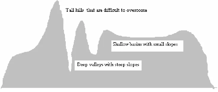
The surfaces of nonlinear objective functions are terrains with both hills and valleys and flat basins as depicted in Fig. 2.1 (Shang, 1997). These terrains pose challenges to any search algorithm because of the differing slopes they offered. Steep slopes of tall hills made them difficult to overcome. Hence once a search get stuck in a local minimum, it would be difficult for the search to get out of it and continue to search for the global minimum. Large shallow basins on the other hand, provide little information for search direction, and may take a long time for a search algorithm to pass these regions if the step-size is inappropriately small (Shang, 1997).
Gradient descent methods are classified as local optimization methods (Shang, 1997). They do not have the ability that guarantees the solutions found are global optima. Thus without a doubt, the basic gradient methods are relatively inefficient when ridges or ravines are salient (Pierre, 1969; Qiu et al., 1992; Ochiai et al., 1994) where most optima reside, be it local or global.
Figure 2.1. The different terrains of the surface of a nonlinear function.
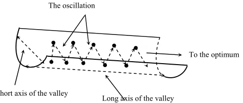
search oscillates back and forth in the direction of the short axis, and only moves very slowly along the long axis of the valley (Rumelhart et al., 1986a; Qian, 1999)
towards the optimal solution. These oscillations make travel time longer and consequently, the slow convergence.
Figure 2.2: The oscillation phenomenon.
Because of this, gradient methods usually show great improvements in the first few iterations but tend to advance slowly as the optimal solution is approached. To further illustrate this phenomenon, consider an objective function with concentric ellipsoidal contours (Ghorbani and Bayat, 2000). If the initial point for a gradient search happens to be precisely on one of the axes of the systems of ellipses, the gradient line will pass right through the optimum and the search will be over in one
descent. Otherwise, the search will follow a zigzag course from p0 to p1 to p2etc.
The following Fig. 2.3 illustrates the situation.
Figure 2.3: The zigzagging phenomenon.
Long axis of the valley Short axis of the valley
To the optimum The oscillation
P1
P0
P5
P2
P3
P4
Furthermore, gradient methods are slow to converge when the surface forms a plane or basin with a gentle slope (Fig. 2.1). This results in too small a gradient to move rapidly over the wide flat surface (Ochiai et al, 1994; Qiu et al, 1992). If one such area is encountered, no significant decrease in the error between two
consecutive terms occurs for some period of time, hence the slow convergence.
This phenomenon might even be mistakenly interpreted as convergence if the error is too insignificant that it is less than the tolerance specified for the algorithm to terminate. If the algorithm terminates, the point of termination is a false optimum. This phenomenon is called ‘premature saturation’ (Fukuoka et al, 1998). However,
if the algorithm does go on and the minimizer is still far away, the error will eventually decrease again. In the end, the algorithm will slowly arrive at the true optimum.
Since gradient methods are local optimizers, the possibility that their solutions are local optima is inevitable. Ravines on the surface in all probability contain local minima, hence a local search procedure that enters such a region, will be directed towards that minimum and stop when it reaches it, while it would be desired that it continue towards a global minimum. This is another instant where the gradient descent methods might be giving false optimum as solutions.
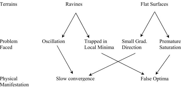
In short, the gradient descent method has the problem of slow convergence that might happen in the vicinities of ravines, ridges, and large flat areas of basins. A secondary problem to these terrains is convergence to local or false optima. Fig. 2.4 summarizes these problems. The DISOPE algorithm being a search method of the gradient descent type, is indisputably susceptible to the same problems. Our aim is to propose methods that can overcome the difficulties.
One of the most prolific algorithms that are based on the gradient descent method is the back propagation algorithm of the neural networks. The area of
this vast volume of knowledge to improve the convergence behavior of DISOPE based on the improvements done to the back propagation algorithm.
Figure 2.4: The schematics of the problems faced by gradient descent algorithms.
2.5 Back Propagation Algorithm
The back propagation algorithm of Rumelhart and McClelland (1986b) is an iterative gradient descent algorithm designed to train multi-layer feed forward networks of sigmoid nodes by minimizing the mean square error between the actual output of the network and the desired output.
Before discussing the back propagation algorithm in detail, some basics of the neural networks are in order. We begin with the description of a perceptron.
2.5.1 A Perceptron
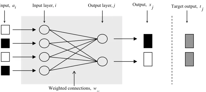
A perceptron is a connected network. The basic perceptron is composed of an input layer and an output layer of nodes as in Fig. 2.5. Each input node is
Terrains Ravines Flat Surfaces
Problem
Faced Oscillation Trapped in Local Minima Small Grad. Direction Premature Saturation
Physical
connected to every output node and vice versa, but there is no connection between nodes in the same layer. Assigned to each connection is a weight. When the first layer sends a signal to the second layer the associated weights are applied on the inputs. The receiving nodes then sum up the incoming values. If the sum exceeds a predetermined threshold, the receiving nodes will fire output signals.
Figure 2.5: A single layer perceptron.
The input of a node i is represented by ai. The input of a node j, Sj, is the
sum of all the weighted inputs from node i. The output of a node j is determined by
the following rule.
0
If then 1
If then 0
n
j i ij
i
j j
j j
S a
S x
S x
θ θ
=
⎫
= ⎪
⎪⎪
> = ⎬
⎪
≤ = ⎪
⎪⎭
∑
w(2.2)
where w is a vector representingall the weights between nodes i and j, n is the
number of nodes in the input layer, and θ is a predetermined threshold value.
The weights can be adjusted so that the network produces a desired output given a set of inputs. The adjusting of weights to produce a particular output is called the training of the network. It is a mechanism that allows the network to learn. The training is accomplished by comparing the actual output xjof the network with a
Input, ai Input layer, i Output layer, j Output, x
j Target output, tj
set of target outputs tj. If there is a difference between the two, the weights are
adjusted to produce a set of outputs closer to the target values. New weights are determined by adding an error correction value to the old weights. The amount of correction is determined by a multiple of the difference between the actual and the target outputs. The multiplier is a constant called a learning rate. The calculation of the new weights can be summed up as follows.
(new) (old) ( )
ij = ij +CN tj−x aj i
w w (2.3)
where CN is the learning rate. The training procedure is repeated until the
performance no longer improves, theoretically when tj =xj.
2.5.2 Multilayer Perceptron
A multilayer perceptron network is a net with one or more layers of nodes between the input and the output units. These extra layers are called the hidden layers. The outputs of one layer are fed-forward as inputs to the next layer. Fig. 2.6 illustrates the architecture of a simple three-layer perceptron. The multilayer
perceptron can solve more complicated problems compared to the single layer perceptron although training may be difficult. The multilayer perceptrons are typically trained using a supervised training algorithm known as the back propagation algorithm.
Figure 2.6: A simple three-layer perceptron.
Inputs Outputs
2.5.3 Representation of the Back Propagation Algorithm
As mentioned earlier, the back propagation algorithm is a gradient descent method aimed at minimizing the total squared error of the output computed by the net. The error function is taken to be the least squares error function below.
∑
=−
= p
j
j
j x
t E
1
2
) (
2 1 )
(w (2.4)
where p is the number of nodes in the output layer. While in training, the weights in
each iteration are changed according to the following rule (Rumelhart and McClelland, 1986).
ij m
ij
E
η ∂
Δ = −
∂
w
w (2.5)
From (2.3) and (2.5) the back propagation algorithm is defined as
( 1) ( )
ij ij m
ij
E n+ = n −η ∂
∂
w w
w (2.6)
where ηm is a small positive number known as the learning rate and n is the iteration
index.
The standard back propagation algorithm inherits the problems of the gradient descent methods. It shows very slow convergence (Moreira and Fiesler, 1995; Fukuoka et al., 1998)and has the tendencyto converge to a false local
minimum (Fukuoka et al., 1998). Over the years, many acceleration techniques have
been developed to speed up the convergence of this algorithm. In the next section, we review some of the better-known approaches that have been documented.
2.5.4 Approaches to Overcome the Slow Convergence