Straight Line And Circular Arc Methods For Developing G 1 And G 2 Involute Curves

Jurnal Teknologi, 43(C) Dis. 2005: 55–66 © Universiti Teknologi Malaysia

STRAIGHT LINE AND CIRCULAR ARC METHODS FOR

DEVELOPING G1 AND G2 INVOLUTE CURVES

R. GOBITHASAN1, R. ROFIZAH2 & M. A. JAMALUDIN3

Abstract. Parametric polynomial curves such as Bezier, Ball, B-splines, Non-uniform B-splines (NURBS) are used for free form curve design. In this paper, we classify these curves as conventional curves. The flexibility of these curves deems suitable for use in the interactive design of curves. On the contrary, these curves cannot be used for highways, railways and robot trajectory designs as the signed curvature of these curves are difficult to control. As a result, the designer has to integrate a time consuming fair process. There are unconventional curves with easy control of the curvature namely, Euler and equiangular spirals. Unfortunately, the formulation of these spirals involves Fresnal integral and exponential functions respectively, which results in extra overhead and implementation. This paper introduces two type of curves which are generated from an evolute-involute process. The first type of evolute-involute curve(s) is generated using straight line(s) as the evolute(s) and named IFSL. The second type of involute curve(s) is generated based on circular arc(s) and a straight line and named IFCA.

Keywords: Computer Aided Geometric Design (CAGD), involute curves, geometric continuity of degree 1 (G1) and 2 (G2), circular arcs, spirals

Abstrak. Lengkung polinomial berparameter seperti Bezier, Ball, splin-B dan Splin-B tak seragam digunakan dalam mereka bentuk lengkung bebas. Dalam kajian ini, kami telah mengkategori lengkung di atas sebagai lengkung konvensional. Fleksibiliti lengkung-lengkung tersebut membolehkannya diguna dalam mereka bentuk lengkung secara interaktif. Namun demikian, lengkung konvensional ini tidak boleh diguna untuk mereka bentuk lebuh raya, landasan keretapi dan trajektori robot kerana kelengkungan bertanda bagi lengkung-lengkung tersebut sukar dikawal. Oleh yang demikian, pereka bentuk harus menerapkan proses saksama yang memakan masa. Terdapat juga lengkung tak konvensional yang mudah dikawal dari segi kelengkungan, misalnya lingkaran Euler dan sama sudut equiangular. Walau bagaimanapun, mereka bentuk lengkung tak konvensional melibatkan kamiran Fresnal dan fungsi eksponen masing-masingnya yang mengakibatkan overhed dan implementasi. Kajian ini memperkenalkan dua jenis lengkung yang dijana melalui proses evolut-involut. Lengkung involut jenis pertama dijana menggunakan garis lurus selaku evolut dan dinamakan IFSL. Lengkung involut jenis kedua dijana berdasarkan segmen bulatan dan garis lurus, dan dinamakan IFCA.

Kata kunci: Reka Bentuk Geometri Dibantu Komputer (RGBK), lengkung involut, keselanjaran geometri berdarjah 1 (G1) dan 2 (G2), segmen bulatan, lingkaran

1

School of Mathematical Sciences, Universiti Sains Malaysia, 11800 Minden, Penang, Malaysia. Tel: +604-653 3924, Fax: +604-657 0910, E-mail: [email protected] or [email protected]

2&3

1.0 INTRODUCTION

The curvature is used as a measure of curve fairness for technical design specifically for aesthetic design, such as car bodies. A curve is said to be fair if it has relatively few curvature monotonous segments [1]. Fair curves are not just important for Computer Aided Design (CAD) and Computer Aided Geometric Design (CAGD) applications, but they play essential roles in highways and robot trajectory designs as well. Inspection of curvature has been used as a passive shape interrogation tool in the field of aesthetic design.

A significant disadvantage of using the conventional curves (Bezier, Ball, B-splines and non-uniform B-splines) is that their curvature is a complicated function of its parameter. Hence, it is not easy to use them in the design of curvature controlled curves. In general, a spiral is said to be a plane curve traced by a point which winds about a fixed pole from which it continually recedes [2]. In CAGD, a spiral is a curve with monotone curvature of constant sign [3]. Two types of spirals which have been widely used in curve design are Euler and equiangular spirals.

The Euler spiral (also called Cornu’s spiral or clothoid) was first studied by Euler in 1781 in connection with an investigation of an elastic spring [4]. The Euler spiral has been used for highways and railways route design [5]. This is because the curvature for clothoid is linearly related to its arc length. The standard clothoid [6] with scaling factor S is:

( ) ( )

( ) 0

C

K S ,

S

θ

θ θ

θ

 

= _{ } ≤

  (1)

where scaled versions of Fresnal integrals C(θ) and S(θ) are:

( ) ( )

0 0

cos sin

0

u u

C du, S du,

u u

θ θ

θ =

_∫

θ =

_∫

≤θ (2)

The equiangular spiral (also called logarithmic spiral) was first discovered by Descartes, followed by its properties of self reproduction by Bernoulli [4]. The radius of curvature of logarithmic spiral is proportional to its arc length. Thus, the task of constructing a smooth planar spline curve with the given end curvature is straightforward using a logarithmic spiral. A logarithmic spiral L(θ) in plane [7] can be defined by:

( ) cos 0

sin

b

L θ r θ , r ae ,θ θ

θ

 

= _{ } = ≤

  (3)

Both Euler and equiangular spirals have their own drawbacks, for instance, clothoid involves integration which is numerically expensive (Simpson rule is widely used for numerical integration). Logarithmic spirals involve exponential, sine and cosine functions and it cannot be represented by a Bezier curve of finite degrees [7]. Thus, researchers look into methods of approximating the spirals by conventional curves [7-9]. A notable research on developing spirals by using cubic Bezier can be seen in [10, 11].

2.0 PROBLEM STATEMENT

The idea of evolutes originated from Huygens [4] in 1673, in conjunction with his studies on light. However, it is said that the concept had existed around 200 BC where it first appeared in the fifth book of Apollonius’s conic sections [4]. Conversely, the idea of involute of a circle was discussed and utilized by Huygens [4] in 1693 in connection with his study of clocks without pendulums for service on ships of the sea. Nowadays, involutes of circle are being used in the design of gear teeth [2].

Involutes can be drawn easily by mechanical means: if a string is attached to a point on a curve, lying along the tangent to the curve at that point and is ‘wrapped up’ on to the curve, the locus of any point of the string is an involute of the given curve [12]. The original curve is called an evolute. A curve can have any number of involutes, thus a curve is an evolute of each of its involutes and an involute of its evolute. The normal to a curve is tangent to its evolute and the tangent to a curve is normal to its involutes. The evolute of a curve is also the envelope of the normal to the curve [13].

The involute of a convex curve in the plane is a spiral in the plane, e.g., the involute of a circle is a spiral (also called anti-clothoid) and the involute of an equiangular spiral is another equiangular spiral.

The idea of using evolute-involute process for curve design was first introduced by Kuroda and Mukai [14] whereby circular arcs have been used as the evolutes to develop G2 involute curves. Recently, Goodman et al. [15] have proposed the generation of an involute spiral that matches G2 Hermite data by means of a polynomial and a rational Pythagorean hodograph as the evolutes.

3.0 A SEGMENT OF IFCA

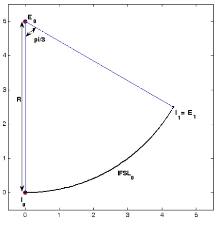
Let a straight line defined from E₀(a₀, b₀) to E₁(a₁, b₁) be the evolute. For simplicity, let E₀ = (0, R₀), where R₀ is the distance from the origin. The length of the stated line is denoted by L₀ and the angle formed between the y-axis and the evolute line by θ₀. By using a trigonometric function, one may produce an involute segment, IFSL₀, denoted by A(θ₀) in the form of a parametric equation with θ₀ as the parameter. The end points are denoted as I₀(x₀, y₀) = (0, 0) and I₁(x₁, y₁) = E₁. Notationwise:

(

)

[

]

(

)

(

)

0 0 0 0 0 1 1 1 1 1 1

E a ,b = ,R , E a ,b = I x , y , (4)

(

)

[ ]

(

)

(

)

0 0 0 0 0 1 1 1 0 sin 0 0 1 cos 0 0 0 2

I x , y = , , I x , y =_R θ ,R − θ _, ≤θ ≤ π (5)

( )

₍

₎

0 0 sin 0 0 1 cos 0 0 0

A θ =_R θ ,R − θ _, ≤ ≤θ θ (6)

From (6), one may generate an involute which is in the form of a circular arc with radius R₀ = L₀. Figure 1 shows an example of generating a IFSL segment with R₀ = 5 and θ₀ = π/3. One may choose a desired θ₀ to design a convex IFSL₀ curve, for instance, if θ₀ = 2π, the resulting IFSL₀ curve is a circle.

4.0 A GENERAL ALGORITHM TO DEVELOP IFSL SPLINE

To generate IFSL_i spline with (n + 1) number of segments where i = 0, …, n, and 0 ≤

θi ≤ 2π, we need to calculate the evolutes of a straight line. For now, consider

0 0 n i i R L =

=

∑

(see Remark 1). The interpolating point of the evolutes can be defined

recursively as:

(

)

1 1 1

0 0

sin cos

n n

i i i i i i i i i

i i

E₊ a₊ ,b₊ a L θ ,b L θ ,

= =

     

= +   −_  _

     



∑

∑

 (7)

Next, the end points of involutes are determined by letting R_i+1= R_i – L_i as:

(

)

1 1 1

0 0

sin cos

n n

i i i i i i i i i

i i

I₊ x₊ , y₊ a R θ ,b R θ

= =       = +   −_  _       

∑

∑

 (8)

Finally, for i= 1, …, n, IFSL_i spline is defined as:

( )

_[

_]

1

0 0

sin , cos where

n n

i i i i i i i

i i

A θ a R θ b R θ , θ θ θ

−

= =

= + −

∑

≤ ≤

∑

(9)

The signed curvature of IFSL_i spline, κ(θ) is calculated as:

( ) ( ) ( )

( )3

1 ' '' i i i ' _i i A A R A θ θ κ θ θ ×

= = (10)

where the symbol × represents the two-dimensional cross product .The norm or

length of A'i( )θ is denoted as Ai'( )θ . Equation (10) proofs that IFSL spline consists

of circular arcs (the curvature of a circular arc is constant).

Remark 1: If the major radius, 0 0 n

i i

R L ,

=

=

∑

then the generated IFSL segments are

joined with geometric continuity of degree 1, GC1, and E_n+1= I_n+1. If ₀

0 n i i R L = >

∑

(or ₀

0 n i i R L =

<

∑

), then the generated segments may not be G1 (a cusp may occur)

and E_n+1 ≠ I_n+1. As a result, it is advisable to fix ₀

0 n i i R L =

We developed a package using MATLAB®7.0 to design IFSL spline interactively. By default, θi is set to be 10 degree and Li is set with a uniform length: Li =R0/n+1. Figure 2 illustrates four examples of developing IFSL spline with 20 segments when R₀ = 30.

Figure 2(a) shows an example of IFSL spline generated using default values θi of

and L_i. Each IFSL segment is G1, it shares the same interpolating point and tangent vectors at the joint. Figure 2(b) (and Figure 2(c)) shows the resulting IFSL spline

(d)

(a) (b)

(c)

when 0 0 n

i i

R L

=

>

∑

(and ₀

0 n

i i

R L

=

<

∑

). Figure 2(d) shows an example of curve design

using θ₃= π/2.

As a result, the designer may implement the proposed algorithm to design a family of convex splines by varying the values of θ_i and L_i, where 0 ≤θ_i≤ 2π and

0 0 n

i i

R L .

= =

∑

5.0 A SEGMENT OF IFCA

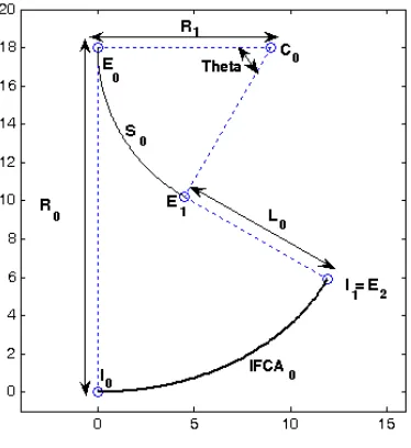
In this section, the construction of a IFCA spiral segment (denoted as B(θ) in parametric form) is shown. Figure 3 illustrates a IFCA₀ spiral.

Figure 3 IFCA0 spiral segment

Let a circular arc be defined from E₀(a₀, b₀) to E₁(a₁, b₁) and a straight line from E₁(a₁, b₁) to E₂(a₂, b₂) be the evolute, where E₀ = (0, R₀). The length of the evolute line is denoted as L₀, the length of the circular arc segment is denoted as S₀ and the angle of the segment is denoted as θ₀. The properties of IFSL₀ spiral segment are defined as:

(

)

[

]

(

) (

)

0 0 0 0 0 0 0 0 1 0

E a ,b = ,R , C p ,q = R ,R , (11)

(

)

[

]

1 1 1 0 0 cos 0 0 0 sin 0

(

)

[

]

1 1 1 1 0 sin 0 1 0 cos 0

I x , y = a +L θ ,b −L θ , (13)

where L₀= R₀– S₀, S₀ = R₁θ₀ and 0 ≤θ₀≤ 2π. Hence, IFSL₀ is defined as:

( )

₍

_{) (}

₎

₍

_{) (}

₎

0 0 1cos 0 1 sin 0 1sin 0 1 cos 0

B θ =_ p −R θ + R −Rθ θ, q −R θ − R −Rθ θ _, (14) where 0 ≤ θ ≤θ₀. Figure 3 shows an example of IFCA₀ spiral segment generated with R₀ = 18, R₁ = 9 and θ₀ = π/3.

The signed curvature of IFSL₀ spiral segment is calculated as:

( )

0 0 1 1 R R κ φ φ =

− ⋅ (15)

where 0 ≤φ ≤θ₀.

6.0 A GENERAL ALGORITHM TO GENERATE SPIRAL SEGMENTS

This section elaborates the algorithm to generate IFSL_i spline with (n+1) segments where i = 1, …, n, and 0 ≤ θi ≤ 2π. A necessary condition is 0

0 n

i n

i

R S L

=

 

=_{ }+



∑

 ,

where S_i = R_i+1θ_i and L_i = L_i–1 – S_i. The centre point of the circular arc is are calculated as:

(

)

1

(

1

)

1 1

(

1

)

1

0

cos sin

n n

i i i i i i i i i i i

i i

C p ,q p R R θ ,q R R θ

− − − + − + =      =_ − − _{ } − − _{ }     



∑

∑

 (16)

where R_i denotes the radius of circular arc (evolute). The interpolating point of the evolutes is calculated as:

(

1 1

)

1 1

0 0

cos sin

n n

i i i i i i i i i

i i

E a₊ ,b₊ p R₊ θ ,q R₊ θ ,

= =

    

=_ − _{ } − _{ }

    



∑

∑

 (17)

The interpolating point of the IFSL_i spiral segment is calculated as:

(

)

1 1 1 1 1

0 0

cos sin

n n

i i i i i i i i i

i i

I₊ x₊ , y₊ a₊ L θ ,b₊ L θ ,

= =

    

=_ + _{ } − _{ }

    



∑

∑

 (18)

( )

(

)

(

)

(

11

)

(

11 11

)

cos sin

sin cos

T

i i i i

i

i i i i

p R L R

B ,

q R L R

θ φ θ

θ

θ φ θ

+ − +

+ − +

− + − ⋅

 

=  _{− − − ⋅} 

 

(19)

where 1

0 0

n n

i i

i i

θ θ θ

−

= =

≤ ≤

∑

∑

and 0≤ ≤φ θ_i.

Upon algebraic simplification, the parametric equation of κ(θ), can be written in a simple form, where 0≤ ≤φ θ_i:

( )

1 1

1

i

i i

L R

κ φ

φ

− +

=

− ⋅ (20)

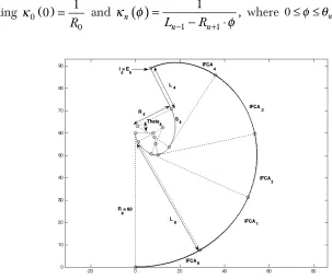
Figure 4 illustrates an example of IFCA spline generated with 5 IFCA spiral segments with:

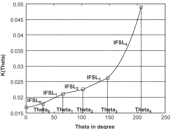
{θ₀, θ₁, θ₂, θ₃, θ₄} = {π/6,π/5,π/5,π/4,π/3}, {R₁, R₂, R₃, R₄, R₅} = {8, 13, 5, 8, 17} and R₀ = 60. The curvature plot (κ(θ) against parameter θ_i) illustrated in Figure 5 indicates that IFCA segments consist of spirals with monotonic increase of positive signed curvature. To note, IFCA spiral segments are joined with GC2 as these pieces share signed curvature values at I_i+1. The designer may fix the end curvatures by defining ₀( )

0

1 0

R

κ = and

( )

1 1

1

n

n n

,

L R

κ φ

φ

− +

=

− ⋅ where 0≤ ≤φ θn.

7.0 CONCLUSION

A general algorithm to develop G1 IFSL and G2 IFCA has been shown in this paper. The IFSL and IFCA splines consist of circular arcs and spirals respectively. These curves can be used for free form curve design, e.g., railways and highways design and robot trajectories where the signed curvature of proposed curves can be controlled to a certain extent. Future work would include identifying the necessary and sufficient conditions that can be matched for a given G2 Hermite data.

ACKNOWLEDGEMENTS

The first author would like to acknowledge KUSTEM for sponsoring his PhD studies at USM. The authors would also like to thank KUSTEM for providing MATLAB® 7.0 which was utilized for this research.

REFERENCE

[1] Farin, G., and N. Sapidis. 1989. Curvature and the Fairness of Curves and Surfaces. Computer Graphics & Application. 9 (2): 52-57.

[2] Lockwood, E. H. 1961. A Book of Curves. Cambridge, England: Cambridge University Press. [3] Davis, P. J. 1993. Spirals: From Theodorus to Chaos. Massachusets: AK Peters Ltd.

[4] Yates, R. C. 1974. Curves and Their Properties. USA: The National Council of Teachers of Mathematics. [5] Bass, K. J. 1984. The Use of Clothoid Templates in Highway Design. Transportation Forum. 1: 47-52. [6] Meek, D. S., and D. J. Walton. 2004. A Note on Finding Clothoid. Journal of Computational and Applied

Mathematics. 170: 433-453.

Figure 5 Curvature plot of IFSL spline

K(Theta)

Theta in degree

0 50 100 150 200 250

0.045 0.05

0.02

0.015 0.025 0.03 0.035 0.04

IFSL₀

Theta₀

IFSL₁

IFSL₂

IFSL₃

IFSL₄

[7] Farin, G., and C. Baumgarten. 1997. Approximation of Logarithmic Spirals. Computer Aided Design. 14: 515-532.

[8] Wang, L. Z., K. T. Miura, E. Nakamae, T. Yamamoto, and T. J. Wang. 2001. Approximation of the Clothoid Curve Defined in the Interval [0, π/2] and its Offset by Free-Form Curves. Computer Aided Design. 33: 1049-1058.

[9] Reyes, J. S., and J. M. Chacon. 2003. Polynomial Approximation to Clothoids via S-power Series. Computer Aided Design. 35: 1305-1313.

[10] Walton, D. J., and D. S. Meek. 1996. A Planar Cubic Bezier Spiral. Journal of Computational and Applied Mathematics. 72: 85-100.

[11] Walton, D. J., D. S. Meek, and J. M. Ali. 2003. Planar G2 Transition Curves Composed of Cubic Bezier Spiral Segments. Journal of Computational and Applied Mathematics. 157: 453-476.

[12] Cundy, H. M., and A. P. Rollett. 1961. Mathematical Models. Oxford: The Clarendon Press. [13] Low, D. A. 1948. Practical Geometry and Graphics. Great Britain: Longmans, Greens and Co. Limited. [14] Kuroda, M., and S. Mukai. 2000. Interpolating Involute Curves. In A. Cohen, C. Rabut, and L. L.

Schumaker (eds). Curve and Surface Fitting: Saint Malo 1999. Nashville: Vanderbilt University Press 1-8. [15] Goodman,T. N. T., D. S. Meek, and D. J. Walton. An Involute Spiral that Matches G2 Hermite Data in