Multiscale boundary element method for Laplace equation

78: 3–2 (2016) 83–88 | www.jurnalteknologi.utm.my | eISSN 2180–3722 |

Jurnal

Teknologi

Full Paper

M

ULTISCALE BOUNDARY ELEMENT METHOD FOR LAPLACE

EQUATION

Nor Afifah Hanim Zulkefli, Munira Ismail, Nor Atirah Izzah Zulkefli,

Yeak Su Hoe

*

Department of Mathematical Sciences, Faculty of Science,

Universiti Teknologi Malaysia, 81310 UTM Johor Bahru, Johor,

Malaysia

Article history

Received

10 February 2015

Received in revised form

29 October 2015

Accepted

30 October 2015

*Corresponding author

[email protected]

Graphical abstract

Abstract

In this paper, the multiscale boundary element method is applied to solve the Laplace equation numerically. The new technique is the coupling of the multiscale technique and the boundary element method in order to speed up the computation. A numerical example is given to illustrate the efficiency of the proposed method. The computed numerical solutions by the proposed method will be compared with the solutions obtained by the conventional boundary element method with the help of Fortran compiler. By comparison, results show that the new technique use less iterations to arrive at the solutions.

Keywords: Laplace equation; boundary element method; multiscale technique

Abstrak

Dalam kertas kerja, kaedah skala berganda unsur sempadan digunakan untuk menyelesaikan persamaan Laplace secara berangka. Teknik baru adalah gandingan teknik skala berganda dan kaedah unsur sempadan untuk mempercepatkan pengiraan. Contoh berangka diberikan untuk menggambarkan kecekapan kaedah yang dicadangkan. Penyelesaian berangka menggunakan kaedah yang dicadangkan akan dibandingkan dengan kaedah unsur sempadan konvensional dengan bantuan pengkompilasi Fortran. Melalui perbandingan, Hasil Kajian menunjukkan bahawa teknik baru menghasilkan kurang lelaran untuk mencapai penyelesaian.

Kata kunci: Persamaan laplace; kaedah unsur sempadan; teknik skala berganda

© 2016 Penerbit UTM Press. All rights reserved

1.0 INTRODUCTION

Numerical method is a popular subject and the basis of all branches of science and technology. In the past, solving problems numerically often meant a great deal of programming and numerical problems. The solution of Laplace equations is a well-known problem in many fields of science and engineering. Several types of numerical methods exist, each with their advantages and disadvantages. Laplace equation is a second order partial differential equation. This is often written as

, 0 2 2 2

  

 u

dy u d dx

u

d

₍₁₎

The _2 _{operation is called the Laplacian of}

.

u Laplace

equation are the simplest examples of elliptic partial differential equations. The general theory of solution to Laplace equation is known as potential theory. Laplace transform comes into its own when the forcing function in the differential equation starts getting more complicated.

element1 Multiscale the mesh 1

0 1

There are many methods in solving the numerical computation of the Laplace equations such as the Finite Element Method (FEM) and the Boundary Element Method (BEM). The FEM does have similarities to the BEM in that it does use elements and nodes, but on the boundaries only. The FEM is a method of dividing a physical system to be analyzed into smaller pieces while the BEM is derived through the discretization of an integral equation. In the BEM, the discretization is done only at the boundary, and this will result in more efficient computation and easier to be used compared with the FEM [1].

This paper applied the multiscale boundary element method for the numerical solution of the Laplace equation. BEM has been widely used to solve the numerical problems, as it offers an excellent accuracy, efficient in modelling, an independent numerical method and easy mesh generation. This brings about the many advantages for the BEM. However, it suffers from well-known drawbacks with regard to the computational efficiency, since the conventional BEM leads to a linear system of equations with dense coefficient matrix [1]. Moreover, it requires the knowledge of a suitable fundamental solution of differential equation. Problems with inhomogeneities or nonlinear differential equations are not accessible by pure BEM. To overcome this problem, we study on the application of multiscale boundary element method for the numerical solution of the Laplace equations with the help of Fortran. Solving the problem of Laplace equations using Bondary Element Method is more slower since heavily use the numerical integration. Therefore we apply the Multiscale Boundary Element Method that will be able to solve the problems accurately and fast.

2.0 BOUNDARY ELEMENT METHODS

InThe Boundary Element Method (BEM) is an important numerical technique, a method of great efficiency. Boundary value problem for systems of partial differential equations is always been solved using the BEM. BEM is a general numerical method for solving boundary-value or initial-value problems formulated by using of the Boundary Integral Equation (BIE). The dimension reduction in BIE formulations makes the BEM mesh much easier to generate for three dimensional problems or infinite domain problems. As early as 1963 Jaswon and Symm presented a numerical technique to solve Fredholm BIEs, which consisted of discretizing the boundary into a series of small segments (elements). The two dimension potential problem was first formulated in terms of a direct BIE and solved numerically by Jaswon, Symm and Jaswon and Ponter [1].

Besides, the BEM is a semianalytical method and thus is more accurate, especially for stress concentration problems such as fracture of structures and can be applied along with the other domain-based methods to verify the solutions to a problem for which no analytical solution is available. Efficient in modelling, the

ability to reduce the dimension of the problem by one is the principal advantage of the BEM over other numerical methods. This property is advantageous as it reduces the size of the system of the problem, leading to improved computational efficiency [2].

Consider the following Poisson equation governing the potential field



in domain V (either 2D or 3D, finite

or infinite) and S is the boundary of the domain:

, 0 2 _{ }





f in V (2)

where f is a known function in domain V. Firstly must

form an integral equation from the Poisson equation by using a weighted integral equation:

. 0 ) (2 



f w

V

(3)

The fundamental solution G(x,y) of a particular

equation is the weighting function that is used in the boundary element formulation of that equation. The fundamental solution for potential problems satisfies:

, / , , 0 ) , ( ) ,

( 2 3

2 R R y x y x y x

G    





(4)

in which the derivatives are taken at point y, and R2

and _R3 _{indicate the full 2D and 3D spaces,} respectively. While the Dirac _ function



_(x,y)

represents a unit source at the source point x, and )

, (x y

G represents the response at the field point y that

is due to that source.

The Dirac  function



(x,y) in 2D and 3D has

following sifting properties:



_ _{ } _

V x V S

V x x f y dV y x y f if , 0 if ), ( ) ( ) , ( )

(



(5)

. . if , 0 if , ) ( ) ( ) , ( ) (



             V i

i _{x V S}

V x x x f y dV x y x y

f



(6)

The fundamental solution G(x,y) is given by:

             , dimensions for three , 4 1 , dimensions for two , 1 log 2 1 ) , ( r r y x G





(7)

where r is the distance between the source point x

and field point y, and its normal derivative is:

             , dimensions for three ), ( 4 1 , dimensions for two ), ( 2 1

2 _y n y

r r y n y r k k k k





(8)

Then use the Green-Gauss theorem. The multi-dimensional equivalent of integration by parts is the Green-Gauss theorem:



2 2



_dS,

n u v n v u dV u v v u S

V







           

(9)

for any two continuous functions u and v, where n is

the component of the outward normal.

Let v(y)



(y), which satisfies Equation (2), and ),

, ( )

(y G x y

u  which satisfies Equation (4). From

Equation (9), we have:







   V y dV y x G y y y x

G( , ) 2



( )



( ) 2 ( , ) ( )

_{( ).} ) ( ) , ( ) ( ) ( ) ( ) ,

( dS y

y n y x G y y n y y x G S



          







(10)

Applying Equations (2), (4) and (5), we obtain:







  S y dS y y x F y q y x G

x) ( , ) ( ) ( , ) ( ) ( )

(





(11)

where q n.

 



Equation (11) is the representation integral of the solution



inside the domain V for Equation (2). Once

the boundary values of both



and q are unknown on

S, if needed, Equation (11) can be applied to

calculate



everywhere in V. This is the BIE generally

used as a starting point for boundary elements.

3.0 MULTISCALE BOUNDARY ELEMENT

METHODS

Past studies have demonstrated that all scale-born complexities can be effectively overcome, or drastically reduced by multiscale (multi-resolution, multilevel, multigrid, etc.) algorithms. A wide range of multiscale computational methods is described, emphasizing main ideas and inter-relations between various fields. Often, a combination of several muliscale approaches can benefit one particular problem in many different ways [3]. An example of a combination of muliscale approaches is by Silvan-Cardenas and Wang, 2006 who has investigated using the multiscale Hermite transform as an approach to separate terrain

elevations from feature heights. Another work was by Aanonsen and Eydinov, 2006 who has investigated a multiscale method was proposed for more-effective history matching of petrophysical properties. While Bovolo et al, 2007 who has established a multiscale technique for reducing the impact of residual misregistration on unsupervised change detection in very high geometrical resolution images [4].

In this paper we attempts to make use of the conjugate gradient and interpolation as a multiscale technique coupling with BEM. Therefore, this study the application of the multiscale BEM for the numerical computation of the Laplace equation. In BEM, we form a standard linear system of equations

,

b

Ax

₍₁₂₎

where A is the coefficient matrix, x is the unknown

vector and b is the known right-hand-side vector. The

linear system can be solved numerically in many approach. Each with their advantages and disadvantages. However, one of the ideal is to apply multiscale technique. In other words, initially, we discretize the region in bigger mesh which produce small size of linear system. This small linear system can be solved using any method. Using the interpolation technique, we can predict better initial guess solution of higher resolution. Thus, with this better predicted initial solution, we can speed up the whole calculation of large linear system. In order to implement this multiscale concept appropriately, we propose the linear system solution using conjugate gradient method. In other words, conjugate gradient method will give better performance once the initial guess solution is “accurate”. The conjugate gradient methods are effective methods were widely use to solve unconstrained optimization problem

), ( minf x

x

(13)

, )

(x Ax b2

f  

₍₁₄₎

), ( 2 )

(x A Ax b f  T 



₍₁₅₎

where _f:n  is continuously differentiable.

Conjugate gradient methods are iterative methods usually formulated as

,

1 k k k

k

d x

x   



(16)

where _xk _{is a current iterate,}

0 

k



is the step length and k

d is a search direction defines as follows

         _ 0 , 0 , 1 _k d g k g d k k k k k



(17)



   V V x y dV y f y x

where _gk denotes the gradient _f(xk₎ and



k is scalar

(Yuan, 2009).

Conjugacy of the search direction is one of the main properties of conjugate gradient method which is included in theorem 2.1.

Theorem 1

For positive defined quadratic function of the form

, 2

1 )

(x x Qx b x c

f _ T _ T _

(18)

where _, n_,  T ₀

Q Q b

x and c is a real number, the

gradient vectors

 

k

g are mutually orthogonal. That is,

. for , 0 )

(gk Tgi  ik

(19)

Moreover, the search direction vectors are mutually Q-conjugate (Joshi and Moudgalya, 2004). In other words,

. for , 0 )

(dk TQdi  ik

(20)

The basic conjugate gradient method which is designed for quadratic function is as below,

Algorithm 1

Step 1: Set k0 select the initial point x0.

Step 2: 0 ₍ 0_).

x f

g  If _g0 0, stop; go to step 9: else,

set 0 0

g d 

Step 3: _.

k k

k k k

d Qd

g d

T T





Step 4: _xk1_xk_



k_dk.

Step 5: k1_{ (} k1_).

x f

g If gk10, stop; go to step 9.

Step 6: 1 _.

k k

k k k

Qd d

Qd g

T T







Step 7: k 1 k1 k k_.

d g

d    



Step 8: Set kk1; go to step 3.

Step 9: End [7].

This method was first proposed for quadratic function it developed into a method for the general functions. For more details, please refer to Refs. [7].

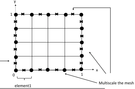
Many different interpolation methods exist. In this paper, we use Piecewise Linear interpolation. This interpolation is the simplest method of getting values at positions in between the data points. The points are simply joined by straight line segments. Each segment that bounded

by two data points can be interpolated independently. Here, we simulate the final results based on the previous computed results. For example, to obtain the result of 8×8 size, we use the initial value from the result 4×4 size.

4.0 NUMERICAL EXAMPLE

Numerical example are presented in this section to demonstrate the accuracy and fast of the multiscale Boundary Element Method for the numerical computation of the Laplace equation compared with boundary element method. All computations were done using Fortran compiler.

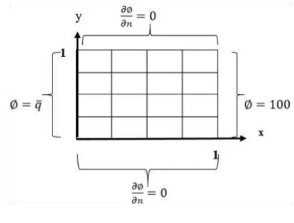
Consider the following the following Laplace equation governing the potential field

_

in domain and

S is the boundary of the domain:

V

in , 0 2 _ 



the boundary conditions to be considered are:

on

, _





 S

(Dirichlet Boundary Condition)

q

S q n

q  , on 







(Neumann Boundary Condition)

in which the over bar indicates the prescribed value for

the function. _{S S S}

q



 is the boundary of the domain

and n is the outward normal of the boundary S. Figure

1 shows the boundary conditions for this example.

Figure 1 Boundary Conditions

Figure 2 Mesh of The Problem

4.1 Results and Discussion

Table 1 and 2 shows the iterations between 4×4, 16×16, 32×32 and 64×64 sizes based on two methods.

Table 1 Iteration Count for Multiscale Boundary Element Method

n size No. of Iterations

4×4 (Initial) 9

4×4



16×16 9 + 39 =48 4×4



32×32 9 + 180 = 189 4×4



64×64 9+443=452

Table 2 Iteration Count for Boundary Element Method

n size No. of Iterations

4×4 9

16×16 62

32×32 217

64×64 463

Table 3 and 4 shows the iterations between 5×5, 20×20, 40×40 and 80×80 sizes based on two methods.

Table 3 Iteration Count for Multiscale Boundary Element Method

n size No. of Iterations

5×5 (Initial) 16

5×5



20×20 16 + 79 = 95 5×5



40×40 16 + 252 = 268 5×5



80×80 16+534=550

Table 4 Iteration Count for Boundary Element Method

n size No. of Iterations

5×5 16

20×20 102

40×40 290

80×80 640

The multiscale Boundary Element Method for solving Laplace problems is presented in this paper. A multiscale technique approach, using a combination of the Conjugate Gradient and interpolation can significantly improve the conditioning of the Boundary Element Method systems of equations and thus can facilitate faster convergence when the multiscale Boundary Element Method is applied.

Based on Table 1 and Table 2, the number of iteration was compared. To compute the result 16×16 size by using the multiscale Boundary Element Method, we need to compute 4×4 size first and then the result is used to compute the solution of 16×16 size. Therefore, the total number of iterations to compute 16×16 size solution is 48 iteration. However, the number of iteration needed to obtain the 16×16 size by Boundary Element Method is 62 iteration. Moreover, the number of iterations for 32×32 and 64×64 sizes by using the multiscale Boundary Element Method is less than Boundary Element Method.

Based on Table 3 and Table 4, the number of iterations for 5×5, 20×20, 40×40 and 80×80 sizes by using the multiscale Boundary Element Method is less than Boundary Element Method. Clearly, the multiscale Boundary Element Method compute the solution faster than Boundary Element Method.

The percentage of iteration reduction can be calculate by using the formula below.

Percentage reduction of iterations

= ([No. of iteration (BEM) – No. of iteration (Propose Method)] / [No. of iteration (BEM)]) x 100%

Table 5 Percentage reduction of iterations

n size Percentage reduction of iterations 4×4



16×16 22.58% 4×4



32×32 12.90% 4×4



64×64 2.38% 5×5



20×20 6.86% 5×5



40×40 7.59% 5×5



80×80 14.06%

Based on Table 5, the percentage of iteration reduction is always positive. We always can obtain the results faster compare to the conventional Boundary Element Method. The schema of initial 5×5 element is more efficient than initial 4×4 element because the initial guess value is close to the exact solution. Piecewise Linear interpolation of 5×5 element can produce better initial guess value.

The numerical example are presented that clearly demonstrate the effiency of the developed the multiscale Boundary Element Method for solving the Laplace Problems.

element1 Multiscale the mesh

1 0

1

5.0 CONCLUSION

Based on numerical result, we conclude that the multiscale Boundary Element Method is faster compared with boundary element method. This paper is expected to establish a numerical library for the solution of the numerical computation of Laplace Equations. For further work, we will simulate more element on boundary. In addition, the numerical results obtained will serve as reference and can be used for validation purposes against other (future) experimental and numerical results. On the other hand, the proposed method can be used as a reference for the future studies in many fields of science and engineering. More research need to be done to improve the Boundary Element Method regarding, for example, convergence of the solvers, optimization of the tree structures, and for dynamic and non-linear problems. Wide spread applications of the Boundary Element Method for solving large-scale engineering problems may not be far away.

Acknowledgement

We acknowledge the financial support from UTM for the Research University Grant (Q.J130000.2626.09J70) and the Ministry of Higher Education (MOHE) in Malaysia.

References

[1] Liu, Y. 2009. Fast Multipole Boundary Element Method - Theory

and Applications in Engineering. Cambridge University Press,

New York.

[2] Grecu, L., and I. Vladimirescu. 2009. BEM with Linear Boundary Elements for Solving the Problem of the 3D Compressible Fluid Flow around Obstacles. Proceedings of the International

MultiConference of Engineers and Computer Scientists

(IMECS) 2009. Hong Kong. 18-20 March 2009. 1-5.

[3] Barth, T. J., T. Chan, and R. Haimes. 2001. Multiscale and

Multiresolution Methods: Theory and Applications. Springer

Verlag, Heidelberg.

[4] Francesca B., L. Bruzzone, S. Marchesi. 2007. A Multiscale Technique for Reducing Registration Noise in Change Detection on Multitemporal VHR Images. Analysis of Multi-temporal Remote Sensing Images, 2007. MultiTemp 2007.

International Workshop. Leuven. 18-20 July 2007. 1-6.

[5] Erhart, K., E. Divo, and A. J. Kassab. 2006. A Parallel Domain Decomposition Boundary Element Method Approach for the Solution of Large-Scale Transient Heat Conduction Problems.

ELSEVIER Engineering Analysis with Boundary Elements. 30(7):

553–563.

[6] Lee Y. and C. Basaran. 2013. A Multiscale Modeling Technique for Bridging Molecular Dynamics with Finite Element Method.

Journal of Computational Physics. 253: 64-85.

[7] Chong E. K. P., and S. H. Zak. 2001. An Introduction to