Technique for Early Reliability Prediction of
Software Components Using Behaviour
Models
Awad Ali1,2*, Dayang N. A. Jawawi1, Mohd Adham Isa1, Muhammad Imran Babar3
1 Department of Information Technology, Faculty of Computer Science, University of Kassala, Kassala, Sudan, 2 Department of Software Engineering, Faculty of Computing, Universiti Teknologi Malaysia, UTM, 81310 Skudai, Johor, Malaysia, 3 Department of Computer Sciences, Army Public College of Management & Sciences Rawalpindi, Pakistan
Abstract
Behaviour models are the most commonly used input for predicting the reliability of a soft-ware system at the early design stage. A component behaviour model reveals the structure and behaviour of the component during the execution of system-level functionalities. There are various challenges related to component reliability prediction at the early design stage based on behaviour models. For example, most of the current reliability techniques do not provide fine-grained sequential behaviour models of individual components and fail to con-sider the loop entry and exit points in the reliability computation. Moreover, some of the cur-rent techniques do not tackle the problem of operational data unavailability and the lack of analysis results that can be valuable for software architects at the early design stage. This paper proposes a reliability prediction technique that, pragmatically, synthesizes system behaviour in the form of a state machine, given a set of scenarios and corresponding con-straints as input. The state machine is utilized as a base for generating the component-rele-vant operational data. The state machine is also used as a source for identifying the nodes and edges of a component probabilistic dependency graph (CPDG). Based on the CPDG, a stack-based algorithm is used to compute the reliability. The proposed technique is evalu-ated by a comparison with existing techniques and the application of sensitivity analysis to a robotic wheelchair system as a case study. The results indicate that the proposed tech-nique is more relevant at the early design stage compared to existing works, and can pro-vide a more realistic and meaningful prediction.
Introduction
Observation of the trends in a range of fields indicates a variety of computer software applica-tions. Computer software can be found embedded in many devices and equipment, such as hand phones, automobiles and aircraft. In addition, software is increasingly used to support critical business applications and industrial processes. Most of these fields depend on software
a11111
OPEN ACCESS
Citation: Ali A, N. A. Jawawi D, Adham Isa M, Imran Babar M (2016) Technique for Early Reliability Prediction of Software Components Using Behaviour Models. PLoS ONE 11(9): e0163346. doi:10.1371/journal.pone.0163346
Editor: Yong Deng, Southwest University, CHINA
Received: October 13, 2015
Accepted: September 7, 2016
Published: September 26, 2016
Copyright:©2016 Ali et al. This is an open access article distributed under the terms of theCreative Commons Attribution License, which permits unrestricted use, distribution, and reproduction in any medium, provided the original author and source are credited.
Data Availability Statement: All relevant data are within the paper.
Funding: The authors received no specific funding for this work.
expected service and is not capable of resuming its service to the state prior to being inter-rupted. Several kinds of failures are possible during service execution, such as faults in the implementation of the software components, hardware failure and network failure. Hardware failure is due to an unreliable hardware resource, and network failure occurs because the mes-sage is lost or there is a problem in inter-component communication [2,3]. Predicting software reliability at an early design stage enables the software’s designer to identify and improve any weak design spots. This is more cost-effective than fixing consequent errors at later implemen-tation phases. Therefore, the reliability technique must be able to work at the early design stage, and particularly during the architectural design phase.
Based on the lifecycle of the reliability measurement, the reliability measures taken early while building and later during the testing or post-deployment [4,5,6]. The data used in these measurements respectively are appraisal data, testing data, and real world data. The purpose of the early measurement is to discover the design spots in order to rework, while later measure-ments are used for the release decision or to certify the components or the whole system. There is no difference in the capability and the property of the reliability approaches that can be used for the two types of the later measurements, because the input data and the purposes are simi-lar. For instance, the later approaches mainly focus on the prediction accuracy while do not pay more attention to the methods of data elicitation and behaviour modeling. Meanwhile, the early approaches concentrate on how to tackle the problem of lack of operational data before the coding stage and the precise modeling of the system behaviour [2,7].
A software development team is a cohesive coalition of individuals working together towards a common goal [8]. The structure of the development team may consist of sub-teams such as design, implementation and deployment team. The members of these sub-teams are requirements analysts, architects, coders, component engineers, testers and so on. The number of the members often depends on the project size and the company policy. For instance, in a small project, the number of the members could be small. Therefore, a team member may have to play a number of roles, either at the same time or in frequent alternation. The early measure-ment of the reliability is part of the design process and stage, therefore, the reliability analysis is conducted as part of the design process [9]. In turn, the later measurements are part of the test-ing process and stage, hence, the analysis is implemented as part of the testtest-ing. The reliability approach in this research is used early as part of the design activities.
Based on behaviour models, several techniques can be used to evaluate the reliability of soft-ware at an early stage and identify the reliability-critical elements of the architecture. However, the existing techniques suffer from a number of drawbacks that limit their applicability and accuracy.
coarse-grained terms are referring to the use of Markov chains directly as a modeling notation to create the architectural models in the form of a state machine. In this sense, system or com-ponent states are represented and interpreted by the state machine, with neither any intermedi-ate notation that reveals the concurrent nature of the system architecture (such as UML, SysML) nor an explicit mechanism that defines how the state machine was constructed.
Second, most of the existing techniques [7,10,11,12] model the influence of the loop entry and exit points on the control and data flow throughout the component behaviour model while neglecting that during reliability computation, because they use Markov model to compute the reliability which assumes the state transition probabilities are history-independent. For example, if a specific set of components’ operations invokes more than another set, because it represents a sequence in a loop, and if these operations have a higher failure rate than the other operations, then computing the reliability without considering the number of invocations will produce an inaccurate prediction. Therefore, the use of technique that is able to keep the previous invoca-tions related values may produce more accurate results. This paper’s work attempts to remedy the shortcomings of the early reliability prediction techniques by proposing a technique for pre-dicting component reliability based on fine-grained sequential models of system architecture synthesized from scenario specifications. This technique is intended to be complementary to the existing approaches of system-level reliability prediction. The values obtained from the pro-posed technique can be used in existing (or future) system-level reliability approaches which require the reliability values of the newly designed components. We argue that dealing with the important challenges in component reliability prediction at the early design stage stems from the precise derivation of an architectural model that is able to reveal the components’ structural and behavioural perspectives, tackle the unavailability of operational data and consider the loop entry and exit points of the behaviour models in the reliability computation.
The paper is structured as follows. We first highlight the research gap in early reliability pre-diction and then discuss the related works in Section 2. Section 3 defines the proposed tech-nique’s elements and construction steps and illustrates the applicability of the proposed technique using an illustrative example. In Section 4, we evaluate and illustrate the applicability of the proposed technique using a real world case study. The last section concludes the paper and provides an outline of future works.
Related Works
During the last decade, many techniques have been proposed to predict software reliability in the early design stage depending on behavioural models; these techniques address different problems and challenges. However, individual component reliability is an integral issue that should be considered in predicting the reliability of a software system at the early design stage [13,14]. Except for certain works [3,10,11,15], which we discuss in this section, most of the cur-rent approaches [6,16,17,18,19,20,21,22,23,24] predict the reliability of a system based on the reliability of its components, without going into sufficient detail about the internal behaviours of the components with respect to down-to-up prediction. It appears that these works assume the availability of the operational data related to individual components. The operational data can be used to determine component reliability accurately without considering a component’s internal structure and behaviour; however, sometimes such information is not available at the early design stage (e.g.in the case of brand new components).
developing a representative operational profile that tackles the lack of knowledge about the new component’s operational data at the early design stage. The profile is built based on the domain expert and operational data obtained from similar functional component(s). In the same way, the work by [7] addresses the problem of individual component reliability predic-tion at the early design stage and the operapredic-tional data unavailability. Furthermore, the author modifies the operational profile devolved in [11] by using multiple information sources that can be available at the early design stage, such as the requirements specification document and a simulation technique in order to achieve more accuracy. The adoption of the work in [7] as part of the system-level reliability approaches [12,25] demonstrates the need for the prediction of individual component reliability in order to predict the whole system reliability. The compo-nent reliability techniques in [11] and [7] mapped the component’s states to a first-order dis-crete-time Markov chain (DTMC) in order to compute the reliability. However, the first-order DTMC does not explicitly reflect the effects of architectural features such as loops and condi-tional branching in the component reliability prediction [12]. Moreover, none of these tech-niques use a fine-grained method that utilizes the explicit requirements specification as the main source at the early design stage to synthesize the behaviour models. The scenario-based method of Rodrigues et al. [10] is perhaps closest in spirit to our own technique. In that work, the behaviour model of the component is synthesized from the requirements specification. The requirements are provided in scenarios using message sequence charts (MSCs). Then, the states of the behaviour model are mapped to the DTMC to compute the reliability. However, that work did not consider the influence of loop entry and exit points in the computation, due to the use of the DTMC.
Proposed Technique for Component Reliability Prediction
The reliability of a component is predicted based on the component’s architectural design and the operational data relevant to this design. The component architectural design is modeled or constructed in the form of a state machine. This state machine can be derived from the code using induction algorithms or from the requirements specification using behaviour synthesis algorithms. This paper’s work is intended for the early design stage before the coding stage; therefore, the proposed technique is built through the behaviour synthesis. Synthesizing a behaviour model or deriving a state machine from requirements specification is the starting point for the proposed technique.
purposes: as a simulation of the component behaviour and as a source for obtaining and identi-fying the elements of a probabilistic dependency graph. The simulation provides an execution log for the component, and the log serves as the runtime observation data required as input to generate operational data for the component. The operational data are necessary to determine the values of the dependency graph’s parameters. Finally, the constructed graph (which is a component probabilistic dependency graph (CPDG)) is used as input to a tree transversal algo-rithm which works to compute the component reliability.
A dependency graph is selected to represent the component structure and behaviour for two reasons. First, it facilitates the capture and modeling of an individual component’s behav-iour (including the loop entry and exit points) and includes the consideration of that informa-tion in the reliability computainforma-tion. This aspect is overlooked in most current component reliability techniques. Second, it is typical to use a specific computation algorithm, namely, the tree transversal algorithm, to allow for a tractable solution.
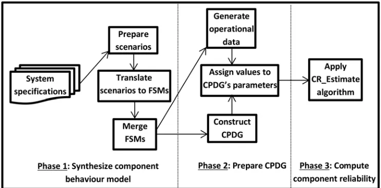
3. Phase 1: Synthesizing the component behaviour model
The process of synthesizing the component behaviour from scenario specifications as a popular requirements elicitation tool involves three activities: preparing scenarios, translating the com-ponent instances in each scenario to FSMs, and merging the FSMs of each comcom-ponent into one state machine model such as the labelled transition system (LTS). In order to define how the behaviour models can be synthesized, this section briefly reviews our previous research work [26], which is relevant to the synthesis of behaviour models from requirements specification; noting that the technique proposed in this paper is not dependent only on our previous work. Any behaviour model that is obtained through one of the existing behaviour synthesis methods or even from a component’s code as a result of a reverse engineering process can be used.
3.1.1 Preparing scenarios. Briefly, the system scenarios in this paper’s work were written
using a scenario language called the scalable triggered scenario (s-TSs) language. Triggered sce-nario languages provide syntactic constructs for describing the conditional or causal relations between sequences of actions. Scenarios in a language like live sequence charts, are described in conditional form (called universal form) and existential. In triggered language, scenarios are described in universal form with existential semantics. This type of modeling provides a good Fig 1. Phases of software component reliability prediction.
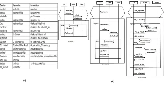
fit with use cases which is the primary form of requirements elicitation. An example of an exis-tential scenario is the automatic teller machine (ATM) scenario which describes a statement like “If the user inserts a valid card into the ATM, and then enters the correct password, she/he shall be able to request cash and have it dispensed by the ATM”. This statement is also condi-tional in the sense that requesting and obtaining cash is expected to be possible if the user has inserted a valid card and input the correct password. An example of a universal statement is: “If the user inserts a valid card into the ATM, and then enters an invalid password, then she/he must receive the password incorrect message”. The s-TSs facilitates the writing of statements like “If the user inserts a valid card into the ATM, and then enters a valid password, then she/ he must able to see the ATM options, otherwise she/he must receive the password incorrect message”. The last statement in a universal form, but more concise and compact (two universal statements combined together). s-TSs use constructs such as implied triggers and branching messages to compact the statements.Fig 2shows the specifications of the ATM system, with
Fig 2(a)depicting the system constraints which are elicited as domain knowledge, andFig 2(b)
illustrating the ATM scenarios using s-TSs.
The s-TSs enhance the current triggered scenario languages [27,28] by adding constructs that enable the writing of scenarios in a compact and concise manner in order to enhance the scalability of scenario modeling. At the early design stage when complete information about the behaviour of a system is not available, there is no option other than to leverage the system constraints and their state variables as basic information sources to enrich system scenarios which are already documented using s-TSs as mentioned previously. The constraints and their state variables (held in a system state vector) are elicited as domain knowledge related to the early design’s specifications. In order to prepare scenarios based on these information sources, in Step 1 we elicit a component’s state variables from the system state vector. The component’s state variables are used to define the constraints relevant to the component’s incoming and Fig 2. System specifications: (a) ATM system constraints, (b) ATM system scenarios using s-TSs.
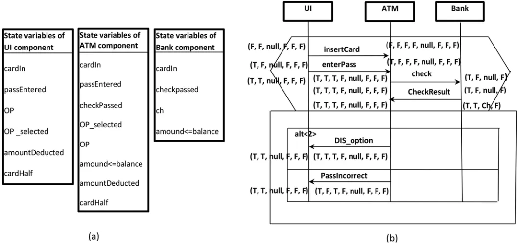
outgoing messages. In Step 2, the values of the component’s state variables which appear in the constraints table (Fig 2(a)) are used to annotate scenarios as pre- and post-conditions associ-ated with each incoming and outgoing message of the component instance. Each component instance is annotated independently, depending on its own state variables list. The reason for this independence is that the goal is only to construct the behaviour model of the component (not the behaviour of the system that represented through the scenario). The values of some state variables may be marked as missing due to not having specifications. Thus, these missing values in the annotated scenarios need to be propagated in Step 3 of this phase using a propaga-tion technique similar to the work by [29] and [30].Fig 3(b)shows one of the scenarios inFig 2
after implementing the scenario preparation steps.
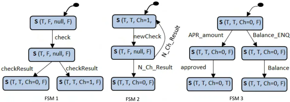
3.1.2 Translating the component instances within the scenario to a set of FSMs. Once
the scenarios are prepared (annotated and propagated), we are ready to synthesize a behaviour model for each component in the system. The strategy starts by generating a number of FSMs for the component (one FSM from each scenario). Thus, each FSM represents the behaviour of the component corresponding to a specific scenario from the set of system scenarios. These FSMs will later be merged (in Phase3) to produce a complete behaviour model of the compo-nent. In order to convert each component instance within a scenario to FSM, pre-post condi-tions values and operacondi-tions (incoming and outgoing messages) of this component instance will be translated to states and transitions, respectively.Fig 4shows the three FSMs of the “Bank” component obtained from the three ATM system scenarios shown previously inFig 2.
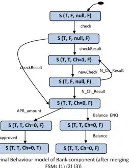
3.1.3 Merging the set of component FSMs into one state machine model.In the final
activity in behaviour model construction, we merge the different FSMs of the component by identifying identical terminal and starting states. Two different FSMs will be merged if and only if the terminal state of one is similar to the starting state of the other. The merging transi-tion will be created from a terminal to a start (the transitransi-tion from a start to a terminal is not allowed). The similarity between the states is determined based on the state vector values of the
Fig 3. Scenario preparation: (a) Elicited state variables of each component in the ATM example, (b) Scenario1 ofFig 2after annotation based on the state variables and propagation.
states. The final output of this phase is the LTS which represents the behaviour of the compo-nent.Fig 5shows the LTS as a result of merging the component FSMs of the “Bank” compo-nent shown above inFig 4.
Phase 2: Preparing a component probabilistic dependency graph
A CPDG is a directed graph that reveals the component’s structure and behaviour, which deter-mine the component’s reliability. The use of a probabilistic graph is a classical method in soft-ware engineering applications. Baah et al. [31] propose a probabilistic graphical model that works with algorithm to analyze program behaviour. This model is used for a program’s fault comprehension and localization. In early reliability prediction there are a number of approaches that use a probabilistic graph. Yacoub et al. [18] proposed a dependency graph with a scenario-based algorithm as a technique to analyze the reliability of a component-scenario-based software system. However, the nodes in Yacoub et al.’s graph representing states of multiple components while CPDG states are belonging to one component, because the purpose in this research is to predict component reliability while in [13] the goal is the whole system reliability.
Preparing the CPDG involves two activities: constructing the CPDG, and generating the operational data. In the construction activity, all the elements of the CPDG are defined based on the basic notation and definitions of the CPDG and the synthesized behaviour model of the targeted component. The synthesis of the behaviour model was already described in relation to the previous phase. The next subsection defines the notations and parameters of the CPDG. Then, the operational data generation activity which provides the data used to assign values to all the CPDG parameters is described.
3.2.1 Constructing the CPDG. Briefly, the CPDG construction requires the identification
of its basic notation and definitions. In graph theory, a directed graph G is defined as a set of pairs, G = (N, E), where:
N represents a set of nodes E represents a set of edges
For CPDG the formal definition is: G = (N, E) where:
N is a finite set of nodes representing the component’s states N = {S, Entry, Exit} where:
S is defined by the tuple<Si,RSi>where:
Siis a unique identification of the component’s states
RSiis the reliability of a state i (it is a probability that indicates that the component will pass
the current state correctly (fault free)
Entry is a virtual state pointing to the first state of the component’s execution (it has no input transition and it reliability is 1)
Exit is a virtual state pointing to the termination of the component’s execution (it has no outgoing transition and it reliability is 1)
E is a finite set of edges representing the transitions between the component’s states E = {T}.
T is defined byPTijorPTiExitwhere:
PTijis the probability of transition from state i to state j, which is the probability that the next
state will be executed after the current state (the sum of the outgoing transition probabilities from each state to all the other states, including implicitly the failure transition, should be 1)
PTiExitis the probability of transition from state i to exit state.
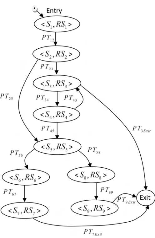
Fig 6shows an example of how a CPDG can be constructed based on the states and
transi-tions of the behaviour model of a component.Fig 6depicts the CPDG of the “Bank” compo-nent which is constructed using the behaviour model of this compocompo-nent. The nodes in the CPDG are directly inherited from the states of the behaviour model, whereby all the states in the behaviour model become nodes in the CPDG. Moreover, “super” nodes Entry and Exit are added to represent the initiation and termination of the execution.
3.2.2 Generating the operational data. The operational data describe the behaviour of the
component quantitatively. The data identify an ordered set of operations that the software component performs along with their associated probabilities. At the early stages of software development, the operational data on a given component may not be available, particularly in the case of newly designed components, and a design time reliability prediction technique must take this uncertainty into consideration. To generate operational data in this paper’s work, the concept of the representative operational profile that has been used in the literature [7,12], relying on a hidden Markov model (HMM) and a Baum–Welch algorithm[32], is adopted. The HMM is defined by four elements’ states S = {S1,S2,S3,. . .,Sn}, a transition matrix
A = {aij}that represents the transition probabilities from state Sito state Sj, observations O =
{O1, O2, O3,. . ., Om}, and an observation probability matrix E = {eik} that represents the
proba-bility of observing event Okin state Si. In this paper’s work, the component behaviour model
that was synthesized in the previous phase will be mapped to define the HMM states S and transition matrix A = {aij}. The observations O and the observation probability matrix E = {eik}
are identified based on the data gathered from similar function components, domain knowl-edge, and analysis of the component architectural model using the technique proposed by [33]. Fig 6. A CPDG constructed from the“Bank” component behaviour model.
Baum–Welch is an iterative optimization technique used with HMM to approximate the best transition and observation probabilities. It is defined as an expectation–maximization algorithm that, given the number of states S, number of observations O, and a set of training data A = {aij}and E = {eik},gives the best values for the transition and observation probability
matrices A and E. In brief, the data obtained from the Baum–Welch algorithm represent the operational data of the component based on the training data, which represent the compo-nent’s behaviour based on its architectural design. However, all these details are relevant to operational profile modeling, which is beyond this paper’s scope. The operational data are uti-lized directly to predict all the CPDG parameters; for instance, if the state Sifails 5 times each
100 execution, it means the reliability of state i is (RSi= 0.95). Similarly, the operational data
give the frequencies of the transitions among the states which translate the transition probabili-ties PTijinto the CPDG.
Phase 3: Computing the component reliability
After constructing the CPDG and defining its related parameters, an algorithm to estimate the component reliability (CR_Estimate) is developed. The algorithm estimates or computes the component reliability based on the CPDG branches and their relevant parameters. In the CPDG, each path represents consecutive states and transitions. The algorithm traverses the CPDG thereby computing the paths’ reliabilities. The computation is based onEq 3, which is derived fromEq 1.Eq 1has been widely used by path-based reliability approaches
[20,34,35,36] at the system level, while in this technique it is adopted at the component level. This adoption is similar to most of the state-based component reliability prediction tech-niques [7,11,12], which reuse a system-level formula at the component level. The CR_Esti-mate algorithm takes the CPDG and the components’ maximum expected iteration number as inputs (as the component operates for a long time). Its outputs are the components’ reliabil-ities with the iterations from zero to the maximum expected iteration number. As with the depth first searching algorithm, CR_Estimate traverses all the CPDG paths from Entry to Exit. Each path is iterated until the number of iterations equals the maximum number of expected iterations. The algorithm at each cycle of the computation refers to the number of the iteration and this determines the termination; therefore, in CR_Estimate, infinite loops that lead to deadlock are not allowed.
By adopting the formula in [35] the path reliability can be defined as:
RPk¼
Yn
i¼1
RSPrðviÞ
i ð1Þ
where:
Rpkis the reliability of the path numberkwherek= 1, 2,. . ., K.
Kis the total number of paths.
nis the number of states in the path.
Pr(vi) is the probability of visiting each state i belonging to the path from the initial state.
From the CPDG definitions, the probability of transition to the first state is 1; then Pr(vi) can
be rewritten as:
PrðviÞ ¼1:PT1;2:PT2;3:. . .:PTi 2;i 1:PTi 1;i
¼PT1;2:PT2;3:. . .:PTi 2;i 1:PTi 1;i
¼Y
i
i¼2
PTi 1;i
23).Eq 4is a common way to compute path reliability in most path-based reliability approaches [20,36,37].
Algorithm 1 Component reliability estimation algorithm: CR_Estimate
1. function computRc(Graph CPDG, maximum expected iteration max_it) 2. Initialization: pthTemp = 1,transTemp = 1, it_no = 0; Rtemp = 0; 3. s = Stack.Create;
4. s.push (SI,RSI, it_no, transTemp, pthTemp);
5. WhileStack6¼;do
6. s.pop(Si,RSi,it_no, transTemp, pthTemp);
7. if Si= = Exit {Exit node}
8. Rtemp+ = PthTemp;
9. k++, it_no = 0;
10. else
11. forit_no = 0tomax_itdo
12. for all Sj,RSj2Sisuccessorsdo
13. transTemp=PTi,j;
14. pthTemp= power(RSj,transTemp);
15. s.push(Sj,RSj,it_no + = 1, pthTemp);
16. Ifit_no = = max_it
17. Si= Exit;
18. end if
19. end for
20. end for
21. end if
22. end While
23. Rc=Rtemp/k
24. return Rc
25. end function
Evaluation
states in a component whose modification has a greater impact on improving the component reliability. From this perspective the sensitivity analysis can be shown as a decision support tool for evaluating various design alternatives. Finally, the comparative analysis was conducted to investigate the improvement yielded by the proposed technique with respect to the problems of existing techniques that have been discussed in the introduction of this paper.
Case Study
In the evaluation we used a software component named theavoid-componentwhich is part of the controlling system of a robotic wheelchair system [38]. The wheelchair software is a com-ponent-based system that has been developed by our research group to support research in embedded real-time (ERT) software engineering and rehabilitation robotics. The robotic wheelchair provides mobility for people with a disability and elderly people who are unable to operate the classical wheelchair system. The behaviour of the robot while in motion is highly constrained by the characteristics of reliability attributes and safety criteria. The robotic wheel-chair consists of a motor power platform that is complete with a detector and certain movers, which depend on the suitability and usability to achieve wheelchair functionality. The most common detectors and movers, such as the infrared detector, sonar, laser, fibre optics and oth-ers, are used in the robotic wheelchair system to detect an obstacle and determine the distance. The power driving system is one of the important factors in a robotic wheelchair because the main purpose is to facilitate wheelchair consumer movement, along with other advantages such as driving automatically and avoiding obstacles.
In order to avoid unnecessary complexity, this research focuses mainly on activities that are related to the scenario of obstacle avoidance from the point of view of an avoid-component of a robotic wheelchair. In this scenario, the avoid-component receives adetectObstaclesignal; this obstacle maybe on the left side or the right side. Depending on the position of the obstacle, the system has to activate anobstacleLeftorobstacleRightvariable, which is located in a compo-nent calledSubsumption. As soon as the variable is activated, it has to set a global variable namedavoidActive, and then it has to wait 2 mc for a direction change before returning back to thedetectObstaclestate to repeat all these activities again.
Synthesis of the Behaviour Model of avoid-component
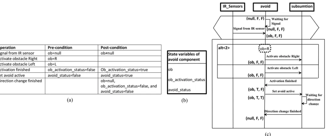
Fig 7(a)shows the wheelchair system constraints as part of the requirements specification.
Based on these constraints and the scenarios of the system, the state variables of the avoid-com-ponent (shown inFig 7(b)) were elicited. Using system constraints and the state variables of the avoid-component, the scenario of obstacle avoidance shown inFig 7(c)is prepared (anno-tated and propagated). By applying the steps defined previously and based on the prepared sce-nario of obstacle avoidance, the behaviour model of the avoid-component is constructed. This behaviour model is shown inFig 8.
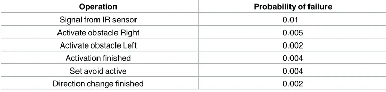
As an illustration, assume that the failure rate values in the behaviour model are related to the operations that appear in the scenario of obstacle avoidance (Fig 7(c)) for which the values are shown inTable 1. Similar to the work by [7,11], as described previously, these values were inferred from analogous components with similar operations and input obtained from a domain expert (the wheelchair developer). The failure rates and the behaviour model are required in the next phase to prepare the CPDG.
Preparation of the CPDG of avoid-component
values of the transition probabilities of the CPDG. The CPDG is constructed through mapping each state and transition in the behaviour model to the node and edge in the CPDG. The super nodes Entry and Exit are added to represent the instantiation and termination of execution.
Fig 9(a)shows the constructed CPDG of the avoid-component.
Fig 7. Part of wheelchair system specifications: (a) System constraints, (b) State vector of avoid-component (elicited based on (a) and the basic scenario of obstacle avoidance), (c) Prepared (annotated and propagated) scenario of obstacle avoidance to synthesize the behaviour model of the avoid-component.
doi:10.1371/journal.pone.0163346.g007
Based on the states of the behaviour model and the failure rates shown above inTable 1, the operational data relevant to the avoid-component were obtained. As described previously, the data were generated through construction of a HMM and execution of the Baum–Welch algo-rithm to train the HMM. To build the HMM, sets of state S = {S1, S2, S3,. . ., Sn} and observa-tions O = {O1, O2, O3,. . ., Om}are needed. Therefore, each state in the behaviour model is mapped to a state in S, and each transition is mapped to an observation in O. Similar to the work by [7,11,12], the domain knowledge and similar function components (e.g. the values in
Table 1) are used to obtain the basic information that describes the behavioural transitions.
This information is used as a basis to initialize the values of the HMM. For example, to deter-mine the probability of receiving a signal from the IR sensor, the probability of failure relevant to this operation which is obtained from similar components is used. However, to determine the detail about whether the signal is received from the left or right IR sensor, domain knowl-edge is used. For instance, assume a domain expert mentioned that the signal comes from the Table 1. Failure rate values of operations in the obstacle avoidance scenario.
Operation Probability of failure
Signal from IR sensor 0.01
Activate obstacle Right 0.005
Activate obstacle Left 0.002
Activation finished 0.004
Set avoid active 0.004
Direction change finished 0.002
doi:10.1371/journal.pone.0163346.t001
analyze the sensitivity of the component reliability to the states’ reliabilities. We also investi-gated how different usage scenarios affected the application reliability.
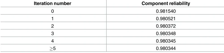
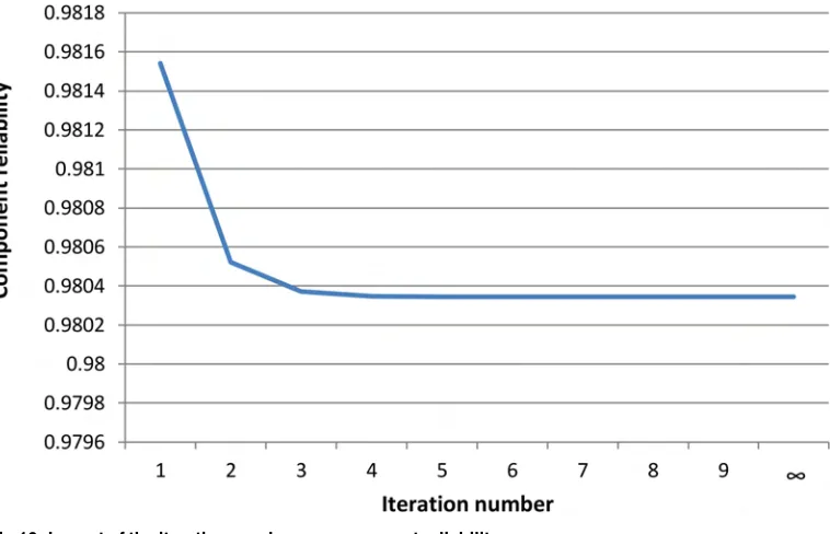
To compute the reliability of the component, we set the maximum iteration number of the algorithm to a large number (in order to reach the steady state probability). Based on the result shown inTable 2andFig 10, it can be seen that the component reliability gradually decreased as the iteration number increased. Thereafter, the component reliability became stable when the iteration number was>4. We can, therefore, report that the reliability at the beginning of the execution was 0.981540, while it decreased and became stable at a value of 0.980344. The iteration number indicates the number of the execution cycle. Based on this result, the reliabil-ity of the avoid-component was 0.980344 which refers to the steady state probabilreliabil-ity of not being in any failure state.
In order to investigate the computational accuracy of the CR_Estimate Algorithm, we need to compare the computed reliability values with measured values of the component. In the early prediction known as the measured reliability value will not be available, due to the absence of runtime information. Furthermore, obtaining a measured value of individual com-ponent reliability is not an easy task. To obtain the reliability of individual comcom-ponent, we need to define all the failure modes caused by the targeted component. Note that the compo-nent usually used as part of other compocompo-nents, therefore it is difficult to determine which com-ponent is causing a specific failure independently. For instance, the avoid-comcom-ponent is part of
Subsumptioncomponent of the wheelchair and some of operations’ execution of the
avoid-component are complemented by an operation that belongs to theSubsumption. Thus, it is dif-ficult to determine whether a specific failure was caused by the avoid-component or other operation in theSubsumption. In fact, as discussed in the introduction of this paper, the absence of the run time information which is used in the component reliability measurement is the main reason that leads to develop the CR_Estimate Algorithm and the related early predic-tion algorithms.
Table 2. Summary of the results of applying CR_Estimate algorithm.
Iteration number Component reliability
0 0.981540
1 0.980521
2 0.980372
3 0.980348
4 0.980345
5 0.980344
Therefore, in the investigation of computational accuracy of the algorithm we will try to measure the difference between the expected and computed reliability value of the component. The expected value can be elicited from information related to analogous components with similar operations and information obtained from a domain expert, such as the information shown inTable 1. The expected value is not a perfect to evaluate the individual component reli-ability, because it is information source that is inherently subjective and may be inaccurate, either due to the complexity of the component or to unexpected operational profiles of that component. However, it is used in this investigation just to give indicator whether the com-puted value is close to the expectation or not with the a help of other related works such as the work presented in the study [7].
If we haveNoperations in the component, andFiis the expected failure probability of the
ithoperation, the expected reliability of the component Ex (Rc) can be elicited by the following
equation:
ExðRcÞ ¼1 XN
i¼1
ðFiÞ ð5Þ
Based onEq (5)and the operation failures of the avoid-component shown inTable 1, it is Ex(Rc) = 0.973. Therefore, the difference between the computed value and the expected is
0.00734. By applying the same way for the algorithm presented in [7], based on the expected operation failures of the used component, the Ex(Rc) = 0.910, while the computed was 0.9223,
so the difference is 0.0123. Based on this simple comparison, our computed value seems more close to the expectation. The purpose of this investigation is just to check whether the accuracy of the computed value is logically acceptable or not. While the main comparison between this research and the related works including the work in [7] will be discussed in the comparison of the results (Section 4.6).
first column.
FromFig 11, it can be observed that the component reliability varied significantly with the
variation in the reliability ofstate1which is related to the receipt of the signal from the IR sen-sor. As the reliability of this state decreased, the component reliability dramatically decreased. This is due to the fact that this state is at the heart of the avoid-component and therefore any faults in this state will easily propagate and affect the correct operation of the component. In addition, from our CPDG shown inFig 9above it can be observed that, as a minimum,state1
will visit twice per each execution cycle. Furthermore,state1belongs to all CPDG paths. On the other hand, the reliability of the component doesn’t vary significantly with the variation in the reliability ofstate3andstate5. This is due to the weak probability of visiting these; for example, the transition probability ofstate3only equals 0.0971. On the contrary, the component reliabil-ity is more sensitive to the reliabilreliabil-ity ofstate2andstate4; this is due to their higher transition probability as compared tostate3. Among the other states,state6andstate7are similar to
state1. Bothstate6andstate7belong to more than one path in CPDG; thus, the component reli-ability is more sensitive to these states than in the case of all other states exceptstate1.The anal-ysis results demonstrate and identify the criticality of each state and the operation that led to it within the avoid-component clearly.
Table 4is the tabular representation of the graph inFig 12. The first column represents
operation failure probabilities. Each of the following columns shows the reliability of the com-ponent when failure probabilities of operation between brackets varies according to the values of the first column.
Fig 12illustrates the impact of varying the operations’ failure probabilities on component
reliability. In each sensitivity run, the failure probabilities of a certain operation were varied between 0 and 0.1, while all other operations remained unchanged. We executed all runs under the obstacle avoidance scenario. As the results in theFig 12show, decreasing the failure proba-bilities generally grew the component reliability linearly. The operationsActivation finished,
Set avoid activewithDirection change finishedhad a similar impact on component reliability, as didActivate obstacle RightwithActivate obstacle Left. Component reliability was particularly sensitive to thesignal from IR sensor, which plays the central role in avoiding an obstacle. The higher impact of this operation is due to the multiple invocations per each path traversal. Hence, it is most beneficial to focus on improving the reliability of thesignal from IR sensor
operation.
a component’s architect to know the effectiveness of the states and the operations quantita-tively. Moreover, sensitivity analyses on the wheelchair demonstrate that the proposed reliabil-ity technique is meaningful and useful from the perspective of making design decisions, as the reliability values obtained are able to aid the architect in evaluating design alternatives.
Comparison of Results
This section investigates the improvement of the proposed technique as compared with the existing works. The investigation was based on a comparison with the related works as dis-cussed above in Section 2. To fairly compare, we chose the three most similar techniques with the proposed technique, as shown inTable 5. The selected techniques were equally compared with the selected comparison criteria regarding early reliability prediction built on the behav-iour model of the components. The comparison criteria were divided into two aspects, namely, the behaviour model and the computational model. The behaviour model aspect reflects the capability of capturing the component structure and behaviour. Moreover, whether the behav-iour model that is used as architecture is fine-grained sequential model or not. On the other Fig 11. Analysis of sensitivity to states’ reliability.
doi:10.1371/journal.pone.0163346.g011
Table 3. Tabular representation ofFig 11. State
reliability
R of comp (state1)
R of comp (state2)
R of comp (state3)
R of comp (state4)
R of comp (state5)
R of comp (state6)
R of comp (state7)
1 0.99825 0.980679 0.980241 0.980579 0.980300 0.980697 0.980439
0.9 0.838993 0.970535 0.977182 0.970453 0.977234 0.967507 0.967289
0.8 0.705382 0.959821 0.973813 0.959762 0.973859 0.953450 0.953276
0.7 0.590883 0.948332 0.970051 0.948300 0.970093 0.938237 0.938110
0.6 0.490741 0.935775 0.965774 0.935776 0.965813 0.921456 0.921383
0.5 0.401277 0.921710 0.960794 0.921754 0.960831 0.902486 0.902474
0.4 0.319424 0.905428 0.954798 0.905525 0.954836 0.880309 0.880370
0.3 0.242353 0.885642 0.947206 0.885807 0.947248 0.853070 0.853220
0.2 0.167019 0.859590 0.936732 0.859848 0.936784 0.816746 0.817014
0.1 0.089282 0.819032 0.919362 0.819433 0.919437 0.759150 0.759600
and consideration of the loop entry and exit points relevant to the behaviour model in the reli-ability computation. The term fine-grained as mentioned in the introduction, according to [10] it refers to the use of a scenario language such as UML SD, MSC or LSC to describe the system scenarios, which have ability to reveal the dynamic behaviour of the system. Then identify an explicit mechanism for transforming these scenarios to state machine formalism such as LTS. Therefore, for any prediction technique if its architecture does not rely on such elements then it can be described as coarse-grained.
The comparison results inTable 5summarize the improvement of the proposed technique against the selected techniques. Apmark in parenthesis means that the technique partially fulfilled the criteria. For the behaviour model aspect, the fine-grained criterion was fully sup-ported by the proposed technique and by the technique proposed by Rodrigues et al. [10], but was neglected in the techniques proposed by Roshandel et al. [40] and Cheung et al. [25]. These two techniques represented the behaviour model of software as a provided state machine without showing how this model was derived from the requirements specification. In our tech-nique and in the techtech-nique proposed by Rodrigues et al., the behaviour model is derived step by step in a precise way from the requirements specification using algorithm presented in our
previous work [24] and discussed briefly in this paper. On the other hand, all the techniques rely on the structure and behaviour of the design specifications but this is partially included in Roshandel et al.’s and Cheung et al.’s works, where the scenario specifications as a primary source for identifying a dynamic behaviour of the system did not appear or were not explicitly used. As for the data availability criterion, most of the approaches provided a mechanism for generating the operational data except for the work by Rodrigues et al. which assumed the availability of such data. Only the proposed technique considered the loop entry and exit points in the computation using a stack-based algorithm; the other techniques used the DTMC to compute the reliability, which does not provide support for such factors.
From the comparison result inTable 5, in summary, the proposed technique is able to reveal the component’s structure and behaviour and provides fine-grained sequential models to be used as the base for reliability prediction. It depends on the requirements specification as input, which is a main source and can be available at the early design stage. The proposed tech-nique takes into account the loop entry and exit points of the behaviour models in the reliabil-ity computation. Moreover, it considers the availabilreliabil-ity of operational data at the early design stage. The inclusion of these factors in the reliability computation can provide a realistic and meaningful evaluation of a component’s reliability. In this sense, the proposed technique shows a strong coupling between the requirements specification, design specifications and computation mechanism during the reliability prediction, which has been overlooked by most of the existing techniques.
Conclusions and Future Work
In this paper, a technique for the early reliability prediction of software components is pre-sented. The proposed technique is shown to have the potential to address the various chal-lenges related to reliability prediction at the early design stage, such as capturing and modeling component behaviour based on the requirements specification. In the proposed technique, a state machine that represents a component’s behaviour is synthesized to reveal the nent’s dynamic behaviour by describing all the possible interaction sequences of the compo-nent. The state machine is utilized as a base to generate the component-relevant operational data with the support of data gathered from similar function components, domain knowledge, the HMM, and the Baum–Welch algorithm. Moreover, the state machine is mainly used as a source for identifying the nodes and edges of a probabilistic dependency graph, called the CPDG. The generated operational data are used to identify the values of the CPDG parameters. Component reliability is computed through a tree transversal algorithm called the CR_Esti-mate which utilizes the CPDG as input.
The requirements specification of an ATM system was used to illustrate the applicability of the proposed technique. A case study for the control system of a robotic wheelchair system was used to evaluate the proposed technique. The evaluation results of applying CR_Estimate in the case study indicate that the proposed technique provides meaningful reliability prediction Table 5. Reliability prediction in design-time techniques.
Technique Behaviour model Computational model
Structure and behaviour Fine-grained Data availability Loops
Rodrigues et al.[10] p p × ×
Roshandel et al.[40] (p) × p ×
Cheung et al. [25] (p) × p ×
Proposed technique p p p p
the operational profile that predicts the transition probabilities among the components’ states through incorporating other machine learning techniques such as the hierarchal hidden Mar-kov model[41]. Furthermore, to broaden the applicability of the proposed technique to differ-ent application domains, our future work intends to apply it to a large number of compondiffer-ents whose detailed requirements specifications are available. Another improvement related to the failure assumption in our work is that there is a possibility that the component might recover from the failure and successfully finish the task’s execution; such a consideration can be included in future work.
Acknowledgments
The authors would like to thank the Associate Editors and anonymous reviewers for their insightful comments and suggestions. The authors are grateful to University of Kassala, Uni-versiti Teknologi Malaysia and the members of the Embedded & Real-Time Software Engineer-ing Laboratory for their feedback and continuous support.
Author Contributions
Conceptualization: AA DNAJ MAI.
Data curation: AA.
Formal analysis: AA.
Investigation: AA DNAJ MAI.
Methodology: AA DNAJ MAI.
Resources: AA DNAJ MAI.
Software: AA.
Supervision: DNAJ MAI.
Validation: AA.
Visualization: AA.
Writing – original draft: AA.
References
1. Lyu MR. Software reliability engineering: A roadmap; 2007. IEEE. pp. 153–170.
2. Brosch F, Koziolek H, Buhnova B, Reussner R (2011) Architecture-Based Reliability Prediction with the Palladio Component Model. IEEE Transactions on Software Engineering: 1–1.
3. Reussner RH, Schmidt HW, Poernomo IH (2003) Reliability prediction for component-based software architectures. Journal of Systems and Software 66: 241–252.
4. Roy B, Graham TCN (2008) Methods for evaluating software architecture: A survey. School of Com-puting TR 545: 82.
5. Wohlin C, Runeson P. A method proposal for early software reliability estimation; 1992. IEEE. pp. 156–163.
6. Cukic B (2005) The virtues of assessing software reliability early. Software, IEEE 22: 50–53.
7. Cheung L, Roshandel R, Medvidovic N, Golubchik L. Early prediction of software component reliability; 2008. ACM. pp. 111–120.
8. Katzenbach JR, Smith DK (1993) The wisdom of teams: Creating the high-performance organization: Harvard Business Press.
9. Sehgal R, Mehrotra D (2015) Predicting Faults before Testing Phase using Halstead’s Metrics. devel-opment 9.
10. Rodrigues G, Rosenblum D, Uchitel S (2005) Using scenarios to predict the reliability of concurrent component-based software systems. Fundamental Approaches to Software Engineering: 111–126. 11. Roshandel R, Banerjee S, Cheung L, Medvidovic N, Golubchik L. Estimating software component
reli-ability by leveraging architectural models; 2006. ACM. pp. 853–856.
12. Cooray D, Kouroshfar E, Malek S, Roshandel R (2013) Proactive self-adaptation for improving the reli-ability of mission-critical, embedded, and mobile software. Software Engineering, IEEE Transactions on 39: 1714–1735.
13. Immonen A, Niemela¨ E (2008) Survey of reliability and availability prediction methods from the view-point of software architecture. Software and Systems Modeling 7: 49–65.
14. Cheung RC (1980) A User-Oriented Software Reliability Model. Software Engineering, IEEE Transac-tions on SE-6: 118–125.
15. Koziolek H, Brosch F (2009) Parameter dependencies for component reliability specifications. Elec-tronic Notes in Theoretical Computer Science 253: 23–38.
16. Gokhale SS, Trivedi KS. Reliability prediction and sensitivity analysis based on software architecture; 2002. IEEE. pp. 64–75.
17. Cortellessa V, Singh H, Cukic B. Early reliability assessment of UML based software models; 2002. ACM. pp. 302–309.
18. Yacoub S, Cukic B, Ammar HH (2004) A scenario-based reliability analysis approach for component-based software. Reliability, IEEE Transactions on 53: 465–480.
19. Goswami V, Acharya Y. Method for Reliability Estimation of COTS Components based Software Sys-tems; 2009.
20. Hsu CJ, Huang CY (2011) An adaptive reliability analysis using path testing for complex component-based software systems. Reliability, IEEE Transactions on 60: 158–170.
21. Fan Z, Xingshe Z, Junwen C, Yunwei D. A Novel Model for Component-Based Software Reliability Analysis; 2008 3–5 Dec. 2008. pp. 303–309.
22. Tyagi K, Sharma A (2012) A rule-based approach for estimating the reliability of component-based systems. Advances in Engineering Software 54: 24–29.
23. Kim Y, Choi O, Kim M, Baik J, Kim T (2013) Validating Software Reliability Early through Statistical Model Checking. Software, IEEE PP: 1–1.
24. Palviainen M, Evesti A, Ovaska E (2011) The reliability estimation, prediction and measuring of compo-nent-based software. Journal of Systems and Software 84: 1054–1070.
25. Cheung L, Krka I, Golubchik L, Medvidovic N. Architecture-level reliability prediction of concurrent sys-tems; 2012. ACM. pp. 121–132.
26. Ali A, Jawawi DN, Isa MA (2015) Scalable Scenario Specifications to Synthesize Component-centric Behaviour Models. International Journal of Software Engineering and Its Applications 9: 79–106. 27. Sibay GE, Braberman V, Uchitel S, Kramer J (2013) Synthesizing modal transition systems from
trig-gered scenarios. Software Engineering, IEEE Transactions on 39: 975–1001.
its components; 1997. IEEE. pp. 146–155.
37. Musa Ia AO K (1987) Software reliability: Measurement, prediction, application. New York: McGraw-Hill. 621 p.
38. Jawawi DN, Kamal K, Talab MA, Zaki MZ, Hamdan NM, Mohamad R, et al. (2011) A Robotic Wheel-chair Component-Based Software Development,. In: (Ed.) B DJ, editor. Mobile Robots—Control Archi-tectures, Bio-Interfacing, Navigation, Multi Robot Motion Planning and Operator Training.
39. Isa MA, Jawawi DNA, Zaki MZ (2013) Model-driven estimation approach for system reliability using integrated tasks and resources. Software Quality Journal: 1–37.
40. Roshandel R, Medvidovic N, Golubchik L (2007) A Bayesian model for predicting reliability of software systems at the architectural level. Software Architectures, Components, and Applications: 108–126. 41. Fine S, Singer Y, Tishby N (1998) The hierarchical hidden Markov model: Analysis and applications.