ABSTRACT
SATTERFIELD, STERLING JUSTIN. The Application of Adaptive Model Refinement to Nuclear Reactor Core Simulation. (Under the direction of Paul Turinsky.)
Nuclear reactor design is a complex, iterative process consisting of the integration of multiple independent system designs, resulting in near constant redesign requiring more simulations.
The nature of this processes is perpetually driving designers to improve the time/accuracy
ratio of reactor simulations to help ensure the achievement of the best possible solution. The application of advanced simulation techniques is used by designers to improve their simulation
capabilities. These techniques revolve around two basic approaches, one of which is to integrate
multiple simulation models to create a hybrid model with the hopes of yielding higher fidelity solutions faster; This is the aspiration of Adaptive Model Refinement (AMoR). This work is a
proof of concept for the application of the AMoR method to nuclear reactor neutron simulation,
specifically the integration of NESTLE [1], a few-group diffusion simulator, with a point reactor kinetics solver (PKE-Solver).
The basis for this approach is grounded in the Quasi-Static method [7] [8], expanding on
the concept of the separability of the flux into amplitude-flux shape-functions [6]. Using this idea, a formulation for the separation of the flux and precursor concentrations into
amplitude-spatial factors was created. The relationship between these factors allowed for the calculation of
the spatial factors by NESTLE, the higher fidelity model, and the calculation of the amplitude factors by the PKE-Solver, the lower fidelity model, resulting in a projected 3-D model. Multiple
error metrics were developed to asses the fidelity of this projected model.
Two AMoR approaches were evaluated in this research. One approach involved the creation of a steady-state library containing the shape-factors, which were used in real-time with the
PKE-Solver to generate the projected model. This approach resulted in a maximum locally
normalized flux and precursor concentration error of roughly 12 - 30% and 60 - 65%, respectively, for the transients simulated. A 2 second transient test case and a 120 second transient test case
were evaluated. The second approach, involved updating the shape-factors from the higher
fidelity model, in real time, when the error of the projected model was deemed too large. For the 2 second transient case, 8 shape-factor updates were required, using a PKE-Solver time-step
size of 0.01 seconds, to maintain a maximum flux error of 25%. For the 120 second transient case, only 4 updates were required, using a PKE-Solver time-step size of 0.30 seconds, to maintain a
©Copyright 2013 by Sterling Justin Satterfield
The Application of Adaptive Model Refinement to Nuclear Reactor Core Simulation
by
Sterling Justin Satterfield
A thesis submitted to the Graduate Faculty of North Carolina State University
in partial fulfillment of the requirements for the Degree of
Master of Science
Nuclear Engineering
Raleigh, North Carolina
2013
APPROVED BY:
Dmitriy Anistratov Ilse Ipsen
Paul Turinsky
DEDICATION
BIOGRAPHY
Sterling Satterfield is originally from the small West Texas town of Midland. He is the youngest of five children of Mr. Johnny Satterfield and Mrs. Jeannie Satterfield. After receiving degrees in
ACKNOWLEDGEMENTS
The completion of this project would not have been possible without the assistance of a great many people. First, I would like to thank my advisor, Dr. Paul Turinsky, for his patients and
guidance while over seeing my work through the last two years. I would also like to thank my friend Ross Hays of the Nuclear Engineering Department for the considerable amount of advice
and assistance he has provided me throughout this time. As well, I would like to thank Hermine
Kabbendjian for her hard work and advice over the last two years.
In addition, I would like to thank my friends, family, and girlfriend, Karen Compton, for
keeping me grounded during my time in North Carolina.
I would also like to thank Dr. Wright, Dr. Nelson, Mr. Cameron, as well as countless others of the University of Texas at the Permian Basin without whom I would have never made it this
far in my academic career.
As well I would like to thank my long time friend and mentor David Cox for making the time to feed my scientific, engineering, and business interest and for the sound advice and guidance
he has provided me throughout my college career.
The last person I would like to thank is Mrs. Karen Sullivan. Without her subtle suggestion to enter the regional science fair, my life would have been drastically different.
Finally, I would like to acknowledge the DOE, CASL, and the Dean’s Grant which without
TABLE OF CONTENTS
LIST OF TABLES . . . vii
LIST OF FIGURES . . . xii
Chapter 1 Introduction . . . 1
1.1 Deterministic Simulation Techniques . . . 2
1.1.1 Overview . . . 2
1.1.2 NESTLE . . . 4
1.1.3 PKE-Solver . . . 5
1.2 Advanced Simulation Techniques . . . 6
1.2.1 Overview . . . 6
1.2.2 Adaptive Model Refinement . . . 7
1.2.3 Quasi-static Diffusion . . . 7
Chapter 2 Methodology . . . 10
2.1 Adaptive Model Refinement Method Formulation . . . 10
2.1.1 Output from NESTLE . . . 10
2.1.2 Shape-factor Formulation . . . 12
2.1.3 Output from the PKE-Solver . . . 13
2.1.4 Formulation of the Projected Model . . . 13
2.1.5 Formulation of Verification Calculations . . . 13
2.1.6 Formulation of Error Calculations . . . 15
2.1.7 Component Error Analysis . . . 19
2.1.8 NESTLE Restart Error Analysis . . . 26
2.2 Adaptive Model Refinement Organization . . . 29
2.2.1 Organization of the Steady-state Library Approach . . . 29
2.2.2 Organization of the Active Model Switching Approach . . . 30
Chapter 3 Results . . . 32
3.1 Testing Environment . . . 32
3.2 Test Cases . . . 32
3.3 Verification Calculation Results . . . 44
3.4 Steady-State Library Results . . . 47
3.5 Active Model Switching Results . . . 80
3.5.1 No Switching - 2 Second Transient . . . 80
3.5.2 No Switching - 120 Second Transient . . . 84
3.5.3 Single Update - 2 Second Transient . . . 87
3.5.4 Single Update - 120 Second Transient . . . 91
3.5.5 Active Switching - 2 Second Transient . . . 95
3.5.6 Active Switching - 120 Second Transient . . . 99
Chapter 4 Conclusions and Recommendations . . . .104
REFERENCES . . . .107
APPENDICES . . . .108
Appendix A Test Cases General Behavior (Continued) . . . 109
A.1 2 Second Transient . . . 109
A.2 120 Second Transient . . . 117
A.3 2 Second Transient,βi0.0001 . . . 125
A.4 120 Second Transient, βi 0.0001 . . . 133
Appendix B Steady-State Library Results (Continued) . . . 141
B.1 2 Second Insertion Transient Using the 10 Entry Steady-State Library and the 10 Output Exact Solution . . . 141
B.2 2 Second Insertion Transient Using the 10 Entry Steady-State Library and the 40 Output Exact Solution . . . 158
B.3 2 Second Insertion Transient Using the 25 Entry Steady-State Library and the 10 Output Exact Solution . . . 162
B.4 2 Second Insertion Transient Using the 25 Entry Steady-State Library and the 40 Output Exact Solution . . . 166
B.5 120 Second Insertion Transient Using the 10 Entry Steady-State Library and the 10 Output Exact Solution . . . 170
B.6 120 Second Insertion Transient Using the 10 Entry Steady-State Library and the 40 Output Exact Solution . . . 174
B.7 120 Second Insertion Transient Using the 25 Entry Steady-State Library and the 10 Output Exact Solution . . . 178
B.8 120 Second Insertion Transient Using the 25 Entry Steady-State Library and the 40 Output Exact Solution . . . 182
Appendix C Active Model Switching (Continued) . . . 186
C.1 No Switching - 2 Second Transient . . . 186
C.2 No Switching - 120 Second Transient . . . 191
C.3 Single Update - 2 Second Transient . . . 195
C.4 Single Update - 120 Second Transient . . . 199
C.5 Active Switching - 2 Second Transient . . . 203
LIST OF TABLES
Table A.1 Radial Relative Power Distribution, 2 Second Transient, Rod Position: 141.25 inches - All Rods Out . . . 109 Table A.2 Radial Relative Power Distribution, 2 Second Transient, Rod Position:
127.12 inches . . . 110 Table A.3 Radial Relative Power Distribution, 2 Second Transient, Rod Position:
113.00 inches . . . 110 Table A.4 Radial Relative Power Distribution, 2 Second Transient, Rod Position:
98.88 inches . . . 110
Table A.5 Radial Relative Power Distribution, 2 Second Transient, Rod Position:
84.75 inches . . . 111
Table A.6 Radial Relative Power Distribution, 2 Second Transient, Rod Position:
70.63 inches . . . 111
Table A.7 Radial Relative Power Distribution, 2 Second Transient, Rod Position:
56.50 inches . . . 111
Table A.8 Radial Relative Power Distribution, 2 Second Transient, Rod Position:
42.38 inches . . . 112
Table A.9 Radial Relative Power Distribution, 2 Second Transient, Rod Position:
28.25 inches . . . 112
Table A.10 Radial Relative Power Distribution, 2 Second Transient, Rod Position:
14.13 inches . . . 112
Table A.11 Radial Relative Power Distribution, 2 Second Transient, Rod Position: 0.00 inches . . . 113 Table A.12 Axial Relative Power Distribution, 2 Second Transient, Rod Position: 141.25
inches - All Rods Out . . . 113 Table A.13 Axial Relative Power Distribution, 2 Second Transient, Rod Position: 127.12
inches . . . 113 Table A.14 Axial Relative Power Distribution, 2 Second Transient, Rod Position: 113.00
inches . . . 114 Table A.15 Axial Relative Power Distribution, 2 Second Transient, Rod Position: 98.88
inches . . . 114 Table A.16 Axial Relative Power Distribution, 2 Second Transient, Rod Position: 84.75
inches . . . 114 Table A.17 Axial Relative Power Distribution, 2 Second Transient, Rod Position: 70.63
inches . . . 115 Table A.18 Axial Relative Power Distribution, 2 Second Transient, Rod Position: 56.50
inches . . . 115 Table A.19 Axial Relative Power Distribution, 2 Second Transient, Rod Position: 42.38
inches . . . 115 Table A.20 Axial Relative Power Distribution, 2 Second Transient, Rod Position: 28.25
inches . . . 116 Table A.21 Axial Relative Power Distribution, 2 Second Transient, Rod Position: 14.13
Table A.22 Axial Relative Power Distribution, 2 Second Transient, Rod Position: 0.00 inches . . . 116 Table A.23 Radial Relative Power Distribution, 120 Second Transient, Rod Position:
141.25 inches - All Rods Out . . . 117 Table A.24 Radial Relative Power Distribution, 120 Second Transient, Rod Position:
127.12 inches . . . 117 Table A.25 Radial Relative Power Distribution, 120 Second Transient, Rod Position:
113.00 inches . . . 118 Table A.26 Radial Relative Power Distribution, 120 Second Transient, Rod Position:
98.87 inches . . . 118
Table A.27 Radial Relative Power Distribution, 120 Second Transient, Rod Position:
84.75 inches . . . 118
Table A.28 Radial Relative Power Distribution, 120 Second Transient, Rod Position:
70.63 inches . . . 119
Table A.29 Radial Relative Power Distribution, 120 Second Transient, Rod Position:
56.50 inches . . . 119
Table A.30 Radial Relative Power Distribution, 120 Second Transient, Rod Position:
42.37 inches . . . 119
Table A.31 Radial Relative Power Distribution, 120 Second Transient, Rod Position:
28.25 inches . . . 120
Table A.32 Radial Relative Power Distribution, 120 Second Transient, Rod Position:
14.12 inches . . . 120
Table A.33 Radial Relative Power Distribution, 120 Second Transient, Rod Position: 0.00 inches . . . 120 Table A.34 Axial Relative Power Distribution, 120 Second Transient, Rod Position:
141.25 inches - All Rods Out . . . 121 Table A.35 Axial Relative Power Distribution, 120 Second Transient, Rod Position:
127.12 inches . . . 121 Table A.36 Axial Relative Power Distribution, 120 Second Transient, Rod Position:
113.00 inches . . . 121 Table A.37 Axial Relative Power Distribution, 120 Second Transient, Rod Position:
98.88 inches . . . 122
Table A.38 Axial Relative Power Distribution, 120 Second Transient, Rod Position:
84.75 inches . . . 122
Table A.39 Axial Relative Power Distribution, 120 Second Transient, Rod Position:
70.63 inches . . . 122
Table A.40 Axial Relative Power Distribution, 120 Second Transient, Rod Position:
56.50 inches . . . 123
Table A.41 Axial Relative Power Distribution, 120 Second Transient, Rod Position:
42.38 inches . . . 123
Table A.42 Axial Relative Power Distribution, 120 Second Transient, Rod Position:
28.25 inches . . . 123
Table A.43 Axial Relative Power Distribution, 120 Second Transient, Rod Position:
Table A.44 Axial Relative Power Distribution, 120 Second Transient, Rod Position: 0.00 inches . . . 124 Table A.45 Radial Relative Power Distribution, 2 Second Transient, Rod Position:
141.25 inches - All Rods Out . . . 125 Table A.46 Radial Relative Power Distribution, 2 Second Transient, Rod Position:
127.12 inches . . . 125 Table A.47 Radial Relative Power Distribution, 2 Second Transient, Rod Position:
113.00 inches . . . 126 Table A.48 Radial Relative Power Distribution, 2 Second Transient, Rod Position:
98.88 inches . . . 126
Table A.49 Radial Relative Power Distribution, 2 Second Transient, Rod Position:
84.75 inches . . . 126
Table A.50 Radial Relative Power Distribution, 2 Second Transient, Rod Position:
70.63 inches . . . 127
Table A.51 Radial Relative Power Distribution, 2 Second Transient, Rod Position:
56.50 inches . . . 127
Table A.52 Radial Relative Power Distribution, 2 Second Transient, Rod Position:
42.38 inches . . . 127
Table A.53 Radial Relative Power Distribution, 2 Second Transient, Rod Position:
28.25 inches . . . 128
Table A.54 Radial Relative Power Distribution, 2 Second Transient, Rod Position:
14.13 inches . . . 128
Table A.55 Radial Relative Power Distribution, 2 Second Transient, Rod Position: 0.00 inches . . . 128 Table A.56 Axial Relative Power Distribution, 2 Second Transient, Rod Position: 141.25
inches - All Rods Out . . . 129 Table A.57 Axial Relative Power Distribution, 2 Second Transient, Rod Position: 127.12
inches . . . 129 Table A.58 Axial Relative Power Distribution, 2 Second Transient, Rod Position: 113.00
inches . . . 129 Table A.59 Axial Relative Power Distribution, 2 Second Transient, Rod Position: 98.88
inches . . . 130 Table A.60 Axial Relative Power Distribution, 2 Second Transient, Rod Position: 84.75
inches . . . 130 Table A.61 Axial Relative Power Distribution, 2 Second Transient, Rod Position: 70.63
inches . . . 130 Table A.62 Axial Relative Power Distribution, 2 Second Transient, Rod Position: 56.50
inches . . . 131 Table A.63 Axial Relative Power Distribution, 2 Second Transient, Rod Position: 42.38
inches . . . 131 Table A.64 Axial Relative Power Distribution, 2 Second Transient, Rod Position: 28.25
inches . . . 131 Table A.65 Axial Relative Power Distribution, 2 Second Transient, Rod Position: 14.13
Table A.66 Axial Relative Power Distribution, 2 Second Transient, Rod Position: 0.00 inches . . . 132 Table A.67 Radial Relative Power Distribution, 120 Second Transient, Rod Position:
141.25 inches - All Rods Out . . . 133 Table A.68 Radial Relative Power Distribution, 120 Second Transient, Rod Position:
127.12 inches . . . 133 Table A.69 Radial Relative Power Distribution, 120 Second Transient, Rod Position:
113.00 inches . . . 134 Table A.70 Radial Relative Power Distribution, 120 Second Transient, Rod Position:
98.87 inches . . . 134
Table A.71 Radial Relative Power Distribution, 120 Second Transient, Rod Position:
84.75 inches . . . 134
Table A.72 Radial Relative Power Distribution, 120 Second Transient, Rod Position:
70.63 inches . . . 135
Table A.73 Radial Relative Power Distribution, 120 Second Transient, Rod Position:
56.50 inches . . . 135
Table A.74 Radial Relative Power Distribution, 120 Second Transient, Rod Position:
42.37 inches . . . 135
Table A.75 Radial Relative Power Distribution, 120 Second Transient, Rod Position:
28.25 inches . . . 136
Table A.76 Radial Relative Power Distribution, 120 Second Transient, Rod Position:
14.12 inches . . . 136
Table A.77 Radial Relative Power Distribution, 120 Second Transient, Rod Position: 0.00 inches . . . 136 Table A.78 Axial Relative Power Distribution, 120 Second Transient, Rod Position:
141.25 inches - All Rods Out . . . 137 Table A.79 Axial Relative Power Distribution, 120 Second Transient, Rod Position:
127.12 inches . . . 137 Table A.80 Axial Relative Power Distribution, 120 Second Transient, Rod Position:
113.00 inches . . . 137 Table A.81 Axial Relative Power Distribution, 120 Second Transient, Rod Position:
98.88 inches . . . 138
Table A.82 Axial Relative Power Distribution, 120 Second Transient, Rod Position:
84.75 inches . . . 138
Table A.83 Axial Relative Power Distribution, 120 Second Transient, Rod Position:
70.63 inches . . . 138
Table A.84 Axial Relative Power Distribution, 120 Second Transient, Rod Position:
56.50 inches . . . 139
Table A.85 Axial Relative Power Distribution, 120 Second Transient, Rod Position:
42.38 inches . . . 139
Table A.86 Axial Relative Power Distribution, 120 Second Transient, Rod Position:
28.25 inches . . . 139
Table A.87 Axial Relative Power Distribution, 120 Second Transient, Rod Position:
LIST OF FIGURES
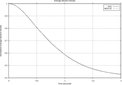
Figure 3.1 Normalzied Volume Averaged Neutron Density . . . 34
Figure 3.2 Normalized Volume Averaged Precursor Concentration (Group: 1) . . . . 35
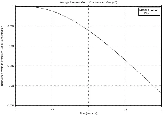
Figure 3.3 Normalized Volume Averaged Precursor Concentration (Group: 2) . . . . 35
Figure 3.4 Normalized Volume Averaged Precursor Concentration (Group: 3) . . . . 36
Figure 3.5 Normalized Volume Averaged Precursor Concentration (Group: 4) . . . . 36
Figure 3.6 Normalized Volume Averaged Precursor Concentration (Group: 5) . . . . 37
Figure 3.7 Normalized Volume Averaged Precursor Concentration (Group: 6) . . . . 37
Figure 3.8 Normalzied Volume Averaged Neutron Density . . . 38
Figure 3.9 Normalized Volume Averaged Precursor Concentration (Group: 1) . . . . 39
Figure 3.10 Normalized Volume Averaged Precursor Concentration (Group: 2) . . . . 39 Figure 3.11 Normalized Volume Averaged Precursor Concentration (Group: 3) . . . . 40 Figure 3.12 Normalized Volume Averaged Precursor Concentration (Group: 4) . . . . 40 Figure 3.13 Normalized Volume Averaged Precursor Concentration (Group: 5) . . . . 41 Figure 3.14 Normalized Volume Averaged Precursor Concentration (Group: 6) . . . . 41 Figure 3.15 Normalzied Volume Averaged Neutron Density . . . 42 Figure 3.16 Normalzied Volume Averaged Neutron Density . . . 43 Figure 3.17 Error Bounds of the Normalized Volume Averaged Neutron Density Error
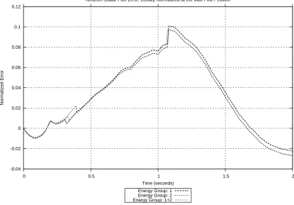
and Locally Normalized Nodal Flux Error at the Maximum Flux Error Position (2 Second Case) . . . 44 Figure 3.18 Error Bounds of the Normalized Volume Averaged Precursor Group
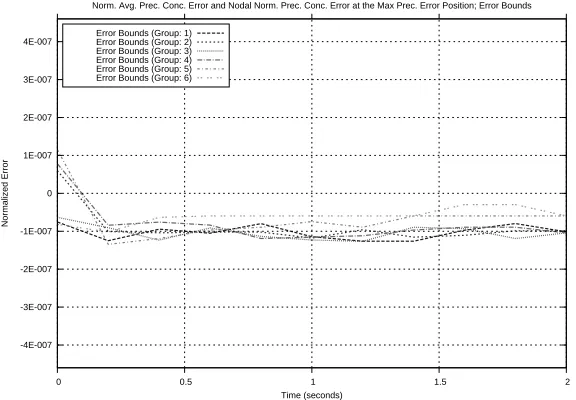
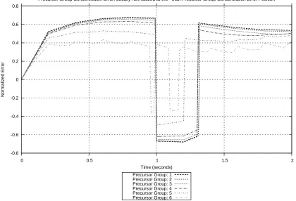
centration Error and the Locally Normalized Nodal Precursor Group Con-centration Error at the Maximum Precursor Group ConCon-centration Error Position (2 Second Case) . . . 45 Figure 3.19 Error Bounds of the Normalized Volume Averaged Neutron Density Error
and Locally Normalized Nodal Flux Error at the Maximum Flux Error Position (120 Second Case) . . . 45 Figure 3.20 Error Bounds of the Normalized Volume Averaged Precursor Group
centration Error and the Locally Normalized Nodal Precursor Group Con-centration Error at the Maximum Precursor Group ConCon-centration Error Position (120 Second Case) . . . 46 Figure 3.21 Locally Normalized Flux Error at the Maximum Flux Position (10 SS, 10
Trans) . . . 48 Figure 3.22 Average Normalized Flux Error at the Maximum Flux Position (10 SS,
10 Trans) . . . 48 Figure 3.23 Locally Normalized Flux Error at the Maximum Flux Error Position (10
SS, 10 Trans) . . . 49 Figure 3.24 Average Normalized Flux Error at the Maximum Flux Error Position (10
SS, 10 Trans) . . . 49
Figure 3.25 Flux L2-Error (10 SS, 10 Trans) . . . 51
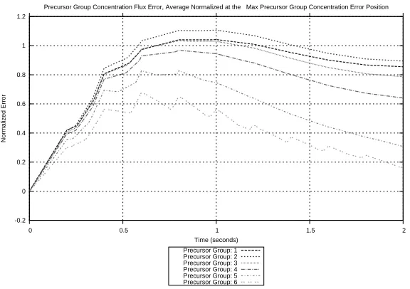
Figure 3.27 Average Normalized Precursor Group Concentration Error at the Maxi-mum Precursor Group Concentration Position (10 SS, 10 Trans) . . . 52 Figure 3.28 Locally Normalized Precursor Group Concentration Error at the
Maxi-mum Precursor Group Concentration Error Position (10 SS, 10 Trans) . . 53 Figure 3.29 Average Normalized Precursor Group Concentration Error at the
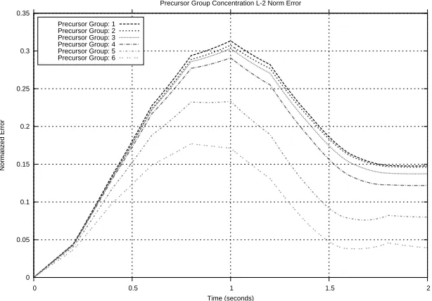
Maxi-mum Precursor Group Concentration Error Position (10 SS, 10 Trans) . . 53 Figure 3.30 Precursor Group Concentration L2-Error (10 SS, 10 Trans) . . . 54 Figure 3.31 Locally Normalized Flux Error at the Maximum Flux Position (10 SS, 40
Trans) . . . 55 Figure 3.32 Locally Normalized Flux Error at the Maximum Flux Error Position (10
SS, 40 Trans) . . . 56 Figure 3.33 Absolute Value of the Locally Normalized Flux Error at the Maximum
Flux Error Position (10 SS, 40 Trans) . . . 56 Figure 3.34 Absolute Value of the Locally Normalized Flux Error and Error
Com-ponents at the Maximum Flux Error Position (10 SS, 40 Trans, Group:
2) . . . 57
Figure 3.35 Locally Normalized Precursor Group Concentration Error at the Maxi-mum Precursor Group Concentration Position (10 SS, 40 Trans) . . . 58 Figure 3.36 Locally Normalized Precursor Group Concentration Error at the
Maxi-mum Precursor Group Concentration Error Position (10 SS, 40 Trans) . . 59 Figure 3.37 Locally Normalized Flux Error at the Maximum Flux Position (25 SS, 10
Trans) . . . 60 Figure 3.38 Locally Normalized Flux Error at the Maximum Flux Error Position (25
SS, 10 Trans) . . . 61 Figure 3.39 Locally Normalized Precursor Group Concentration Error at the
Maxi-mum Precursor Group Concentration Position (25 SS, 10 Trans) . . . 61 Figure 3.40 Locally Normalized Precursor Group Concentration Error at the
Maxi-mum Precursor Group Concentration Error Position (25 SS, 10 Trans) . . 62 Figure 3.41 Locally Normalized Flux Error at the Maximum Flux Position (25 SS, 40
Trans) . . . 63 Figure 3.42 Locally Normalized Flux Error at the Maximum Flux Error Position (25
SS, 40 Trans) . . . 64 Figure 3.43 Locally Normalized Precursor Group Concentration Error at the
Maxi-mum Precursor Group Concentration Position (25 SS, 40 Trans) . . . 64 Figure 3.44 Locally Normalized Precursor Group Concentration Error at the
Maxi-mum Precursor Group Concentration Error Position (25 SS, 40 Trans) . . 65 Figure 3.45 Locally Normalized Flux Error at the Maximum Flux Position (10 SS, 10
Trans) . . . 66 Figure 3.46 Locally Normalized Flux Error at the Maximum Flux Error Position (10
SS, 10 Trans) . . . 67 Figure 3.47 Locally Normalized Flux Error and Error Components at the Maximum
Flux Error Position (10 SS, 10 Trans, Group: 2) . . . 68
Figure 3.49 Locally Normalized Precursor Group Concentration Error at the Maxi-mum Precursor Group Concentration Error Position (10 SS, 10 Trans) . . 69 Figure 3.50 Locally Normalized Precursor Group Concentration Error at the
Maxi-mum Precursor Group Concentration Error Position (10 SS, 10 Trans,
Group 6) . . . 69
Figure 3.51 Locally Normalized Precursor Group Concentration Error and Error Com-ponents at the Maximum Precursor Group Concentration Error Position (10 SS, 10 Trans, Group 1) . . . 70 Figure 3.52 Locally Normalized Precursor Group Concentration Error and Error
Com-ponents at the Maximum Precursor Group Concentration Error Position (10 SS, 10 Trans, Group 4) . . . 70 Figure 3.53 Locally Normalized Flux Error at the Maximum Flux Position (10 SS, 40
Trans) . . . 71 Figure 3.54 Locally Normalized Flux Error at the Maximum Flux Error Position (10
SS, 40 Trans) . . . 72 Figure 3.55 Locally Normalized Precursor Group Concentration Error at the
Maxi-mum Precursor Group Concentration Position (10 SS, 40 Trans) . . . 72 Figure 3.56 Locally Normalized Precursor Group Concentration Error at the
Maxi-mum Precursor Group Concentration Error Position (10 SS, 40 Trans) . . 73 Figure 3.57 Locally Normalized Flux Error at the Maximum Flux Position (25 SS, 10
Trans) . . . 74 Figure 3.58 Locally Normalized Flux Error at the Maximum Flux Error Position (25
SS, 10 Trans) . . . 75 Figure 3.59 Locally Normalized Precursor Group Concentration Error at the
Maxi-mum Precursor Group Concentration Position (25 SS, 10 Trans) . . . 75 Figure 3.60 Locally Normalized Precursor Group Concentration Error at the
Maxi-mum Precursor Group Concentration Error Position (25 SS, 10 Trans) . . 76 Figure 3.61 Locally Normalized Flux Error at the Maximum Flux Position (25 SS, 40
Trans) . . . 77 Figure 3.62 Locally Normalized Flux Error at the Maximum Flux Error Position (25
SS, 40 Trans) . . . 78 Figure 3.63 Locally Normalized Precursor Group Concentration Error at the
Maxi-mum Precursor Group Concentration Position (25 SS, 40 Trans) . . . 78 Figure 3.64 Locally Normalized Precursor Group Concentration Error at the
Maxi-mum Precursor Group Concentration Error Position (25 SS, 40 Trans) . . 79 Figure 3.65 Locally Normalized Flux Error at the Maximum Flux Error Position (No
switch, Trans 40) . . . 81 Figure 3.66 Average Normalized Flux Error at the Maximum Flux Error Position (No
switch, Trans 40) . . . 82 Figure 3.67 Flux L2-Error (No switch, Trans 40) . . . 83 Figure 3.68 Locally Normalized Flux Error at the Maximum Flux Error Position (No
switch, Trans 40) . . . 84 Figure 3.69 Average Normalized Flux Error at the Maximum Flux Error Position (No
Figure 3.70 Flux L2-Error (No switch, Trans 40) . . . 86 Figure 3.71 Locally Normalized Flux Error at the Maximum Flux Error Position (One
update, Trans 40) . . . 88 Figure 3.72 Average Normalized Flux Error at the Maximum Flux Error Position
(One update, Trans 40) . . . 89 Figure 3.73 Flux L2-Error (One update, Trans 40) . . . 90 Figure 3.74 Locally Normalized Flux Error at the Maximum Flux Error Position (One
update, Trans 40) . . . 92 Figure 3.75 Average Normalized Flux Error at the Maximum Flux Error Position
(One update, Trans 40) . . . 93 Figure 3.76 Flux L2-Error (One update, Trans 40) . . . 94 Figure 3.77 Locally Normalized Flux Error at the Maximum Flux Error Position
(Ac-tive, Trans 40) . . . 96
Figure 3.78 Average Normalized Flux Error at the Maximum Flux Error Position (Active, Trans 40) . . . 97 Figure 3.79 Flux L2-Error (Active, Trans 40) . . . 98 Figure 3.80 Locally Normalized Flux Error at the Maximum Flux Error Position
(Ac-tive, Trans 40) . . . 100
Figure 3.81 Average Normalized Flux Error at the Maximum Flux Error Position (Active, Trans 40) . . . 101 Figure 3.82 Flux L2-Error (Active, Trans 40) . . . 102
Figure B.1 Flux Error and Error Components at the Maximum Flux Position Locally Normalized (Group: 1, 10 SS, 10 Trans) . . . 142 Figure B.2 Flux Error and Error Components at the Maximum Flux Position Locally
Normalized (Group: 2, 10 SS, 10 Trans) . . . 142 Figure B.3 Flux Error and Error Components at the Maximum Flux Position
Aver-age Normalized (Group: 1, 10 SS, 10 Trans) . . . 143 Figure B.4 Flux Error and Error Components at the Maximum Flux Position
Aver-age Normalized (Group: 2, 10 SS, 10 Trans) . . . 143 Figure B.5 Flux Error and Error Components at the Maximum Flux Error Position
Locally Normalized (Group: 1, 10 SS, 10 Trans) . . . 144 Figure B.6 Flux Error and Error Components at the Maximum Flux Position Locally
Normalized (Group: 2, 10 SS, 10 Trans) . . . 144 Figure B.7 Flux Error and Error Components at the Maximum Flux Error Position
Average Normalized (Group: 1, 10 SS, 10 Trans) . . . 145 Figure B.8 Flux Error and Error Components at the Maximum Flux Position
Aver-age Normalized (Group: 2, 10 SS, 10 Trans) . . . 145 Figure B.9 Precursor Concentration Error and Error Components at the Maximum
Precursor Concentration Position Locally Normalized (Group: 1, 10 SS, 10 Trans) . . . 146 Figure B.10 Precursor Concentration Error and Error Components at the Maximum
Figure B.11 Precursor Concentration Error and Error Components at the Maximum Precursor Concentration Position Locally Normalized (Group: 3, 10 SS, 10 Trans) . . . 147 Figure B.12 Precursor Concentration Error and Error Components at the Maximum
Precursor Concentration Position Locally Normalized (Group: 4, 10 SS, 10 Trans) . . . 147 Figure B.13 Precursor Concentration Error and Error Components at the Maximum
Precursor Concentration Position Locally Normalized (Group: 5, 10 SS, 10 Trans) . . . 148 Figure B.14 Precursor Concentration Error and Error Components at the Maximum
Precursor Concentration Position Locally Normalized (Group: 6, 10 SS, 10 Trans) . . . 148 Figure B.15 Precursor Concentration Error and Error Components at the Maximum
Precursor Concentration Position Average Normalized (Group: 1, 10 SS, 10 Trans) . . . 149 Figure B.16 Precursor Concentration Error and Error Components at the Maximum
Precursor Concentration Position Average Normalized (Group: 2, 10 SS, 10 Trans) . . . 149 Figure B.17 Precursor Concentration Error and Error Components at the Maximum
Precursor Concentration Position Average Normalized (Group: 3, 10 SS, 10 Trans) . . . 150 Figure B.18 Precursor Concentration Error and Error Components at the Maximum
Precursor Concentration Position Average Normalized (Group: 4, 10 SS, 10 Trans) . . . 150 Figure B.19 Precursor Concentration Error and Error Components at the Maximum
Precursor Concentration Position Average Normalized (Group: 5, 10 SS, 10 Trans) . . . 151 Figure B.20 Precursor Concentration Error and Error Components at the Maximum
Precursor Concentration Position Average Normalized (Group: 6, 10 SS, 10 Trans) . . . 151 Figure B.21 Precursor Concentration Error and Error Components at the Maximum
Precursor Concentration Error Position Locally Normalized (Group: 1, 10 SS, 10 Trans) . . . 152 Figure B.22 Precursor Concentration Error and Error Components at the Maximum
Precursor Concentration Error Position Locally Normalized (Group: 2, 10 SS, 10 Trans) . . . 152 Figure B.23 Precursor Concentration Error and Error Components at the Maximum
Precursor Concentration Error Position Locally Normalized (Group: 3, 10 SS, 10 Trans) . . . 153 Figure B.24 Precursor Concentration Error and Error Components at the Maximum
Figure B.25 Precursor Concentration Error and Error Components at the Maximum Precursor Concentration Error Position Locally Normalized (Group: 5, 10 SS, 10 Trans) . . . 154 Figure B.26 Precursor Concentration Error and Error Components at the Maximum
Precursor Concentration Error Position Locally Normalized (Group: 6, 10 SS, 10 Trans) . . . 154 Figure B.27 Precursor Concentration Error and Error Components at the Maximum
Precursor Concentration Error Position Average Normalized (Group: 1, 10 SS, 10 Trans) . . . 155 Figure B.28 Precursor Concentration Error and Error Components at the Maximum
Precursor Concentration Error Position Average Normalized (Group: 2, 10 SS, 10 Trans) . . . 155 Figure B.29 Precursor Concentration Error and Error Components at the Maximum
Precursor Concentration Error Position Average Normalized (Group: 3, 10 SS, 10 Trans) . . . 156 Figure B.30 Precursor Concentration Error and Error Components at the Maximum
Precursor Concentration Error Position Average Normalized (Group: 4, 10 SS, 10 Trans) . . . 156 Figure B.31 Precursor Concentration Error and Error Components at the Maximum
Precursor Concentration Error Position Average Normalized (Group: 5, 10 SS, 10 Trans) . . . 157 Figure B.32 Precursor Concentration Error and Error Components at the Maximum
Precursor Concentration Error Position Average Normalized (Group: 6, 10 SS, 10 Trans) . . . 157
Figure B.33 Flux L2-Error (10 SS, 40 Trans) . . . 158
Figure B.34 Average Normalized Flux Error at the Maximum Flux Position (10 SS, 40 Trans) . . . 159 Figure B.35 Average Normalized Flux Error at the Maximum Flux Error Position (10
SS, 40 Trans) . . . 159 Figure B.36 Average Normalized Precursor Group Concentration Error at the
Maxi-mum Precursor Group Concentration Position (10 SS, 40 Trans) . . . 160 Figure B.37 Average Normalized Precursor Group Concentration Error at the
Maxi-mum Precursor Group Concentration Error Position (10 SS, 40 Trans) . . 160 Figure B.38 Precursor Group Concentration L2-Error (10 SS, 40 Trans) . . . 161
Figure B.39 Flux L2-Error (25 SS, 10 Trans) . . . 162
Figure B.40 Average Normalized Flux Error at the Maximum Flux Position (25 SS, 10 Trans) . . . 163 Figure B.41 Average Normalized Flux Error at the Maximum Flux Error Position (25
SS, 10 Trans) . . . 163 Figure B.42 Average Normalized Precursor Group Concentration Error at the
Maxi-mum Precursor Group Concentration Position (25 SS, 10 Trans) . . . 164 Figure B.43 Average Normalized Precursor Group Concentration Error at the
Figure B.45 Flux L2-Error (25 SS, 40 Trans) . . . 166 Figure B.46 Average Normalized Flux Error at the Maximum Flux Position (25 SS,
40 Trans) . . . 167 Figure B.47 Average Normalized Flux Error at the Maximum Flux Error Position (25
SS, 40 Trans) . . . 167 Figure B.48 Average Normalized Precursor Group Concentration Error at the
Maxi-mum Precursor Group Concentration Position (25 SS, 40 Trans) . . . 168 Figure B.49 Average Normalized Precursor Group Concentration Error at the
Maxi-mum Precursor Group Concentration Error Position (25 SS, 40 Trans) . . 168 Figure B.50 Precursor Group Concentration L2-Error (25 SS, 40 Trans) . . . 169
Figure B.51 Flux L2-Error (10 SS, 10 Trans) . . . 170
Figure B.52 Average Normalized Flux Error at the Maximum Flux Position (10 SS, 10 Trans) . . . 171 Figure B.53 Average Normalized Flux Error at the Maximum Flux Error Position (10
SS, 10 Trans) . . . 171 Figure B.54 Average Normalized Precursor Group Concentration Error at the
Maxi-mum Precursor Group Concentration Position (10 SS, 10 Trans) . . . 172 Figure B.55 Average Normalized Precursor Group Concentration Error at the
Maxi-mum Precursor Group Concentration Error Position (10 SS, 10 Trans) . . 172 Figure B.56 Precursor Group Concentration L2-Error (10 SS, 10 Trans) . . . 173
Figure B.57 Flux L2-Error (10 SS, 40 Trans) . . . 174
Figure B.58 Average Normalized Flux Error at the Maximum Flux Position (10 SS, 40 Trans) . . . 175 Figure B.59 Average Normalized Flux Error at the Maximum Flux Error Position (10
SS, 40 Trans) . . . 175 Figure B.60 Average Normalized Precursor Group Concentration Error at the
Maxi-mum Precursor Group Concentration Position (10 SS, 40 Trans) . . . 176 Figure B.61 Average Normalized Precursor Group Concentration Error at the
Maxi-mum Precursor Group Concentration Error Position (10 SS, 40 Trans) . . 176 Figure B.62 Precursor Group Concentration L2-Error (10 SS, 40 Trans) . . . 177
Figure B.63 Flux L2-Error (25 SS, 10 Trans) . . . 178
Figure B.64 Average Normalized Flux Error at the Maximum Flux Position (25 SS, 10 Trans) . . . 179 Figure B.65 Average Normalized Flux Error at the Maximum Flux Error Position (25
SS, 10 Trans) . . . 179 Figure B.66 Average Normalized Precursor Group Concentration Error at the
Maxi-mum Precursor Group Concentration Position (25 SS, 10 Trans) . . . 180 Figure B.67 Average Normalized Precursor Group Concentration Error at the
Maxi-mum Precursor Group Concentration Error Position (25 SS, 10 Trans) . . 180 Figure B.68 Precursor Group Concentration L2-Error (25 SS, 10 Trans) . . . 181
Figure B.69 Flux L2-Error (25 SS, 40 Trans) . . . 182
Figure B.71 Average Normalized Flux Error at the Maximum Flux Error Position (25 SS, 40 Trans) . . . 183 Figure B.72 Average Normalized Precursor Group Concentration Error at the
Maxi-mum Precursor Group Concentration Position (25 SS, 40 Trans) . . . 184 Figure B.73 Average Normalized Precursor Group Concentration Error at the
Maxi-mum Precursor Group Concentration Error Position (25 SS, 40 Trans) . . 184 Figure B.74 Precursor Group Concentration L2-Error (25 SS, 40 Trans) . . . 185
Figure C.1 Flux Error and Error Components at the Maximum Flux Position Locally Normalized (No switch, Trans 40, Group: 1) . . . 187 Figure C.2 Flux Error and Error Components at the Maximum Flux Position Locally
Normalized (No switch, Trans 40, Group: 2) . . . 187 Figure C.3 Flux Error and Error Components at the Maximum Flux Position
Aver-age Normalized (No switch, Trans 40, Group: 1) . . . 188
Figure C.4 Flux Error and Error Components at the Maximum Flux Position
Aver-age Normalized (No switch, Trans 40, Group: 2) . . . 188
Figure C.5 Flux Error and Error Components at the Maximum Flux Error Position Locally Normalized (No switch, Trans 40, Group: 1) . . . 189 Figure C.6 Flux Error and Error Components at the Maximum Flux Error Position
Locally Normalized (No switch, Trans 40, Group: 2) . . . 189 Figure C.7 Flux Error and Error Components at the Maximum Flux Error Position
Average Normalized (No switch, Trans 40, Group: 1) . . . 190 Figure C.8 Flux Error and Error Components at the Maximum Flux Error Position
Average Normalized (No switch, Trans 40, Group: 2) . . . 190 Figure C.9 Flux Error and Error Components at the Maximum Flux Position Locally
Normalized (No switch, Trans 40, Group: 1) . . . 191 Figure C.10 Flux Error and Error Components at the Maximum Flux Position Locally
Normalized (No switch, Trans 40, Group: 2) . . . 191 Figure C.11 Flux Error and Error Components at the Maximum Flux Position
Aver-age Normalized (No switch, Trans 40, Group: 1) . . . 192
Figure C.12 Flux Error and Error Components at the Maximum Flux Position
Aver-age Normalized (No switch, Trans 40, Group: 2) . . . 192
Figure C.13 Flux Error and Error Components at the Maximum Flux Error Position Locally Normalized (No switch, Trans 40, Group: 1) . . . 193 Figure C.14 Flux Error and Error Components at the Maximum Flux Error Position
Locally Normalized (No switch, Trans 40, Group: 2) . . . 193 Figure C.15 Flux Error and Error Components at the Maximum Flux Error Position
Average Normalized (No switch, Trans 40, Group: 1) . . . 194 Figure C.16 Flux Error and Error Components at the Maximum Flux Error Position
Average Normalized (No switch, Trans 40, Group: 2) . . . 194 Figure C.17 Flux Error and Error Components at the Maximum Flux Position Locally
Normalized (One update, Trans 40, Group: 1) . . . 195 Figure C.18 Flux Error and Error Components at the Maximum Flux Position Locally
Figure C.19 Flux Error and Error Components at the Maximum Flux Position
Aver-age Normalized (One update, Trans 40, Group: 1) . . . 196
Figure C.20 Flux Error and Error Components at the Maximum Flux Position
Aver-age Normalized (One update, Trans 40, Group: 2) . . . 196
Figure C.21 Flux Error and Error Components at the Maximum Flux Error Position Locally Normalized (One update, Trans 40, Group: 1) . . . 197 Figure C.22 Flux Error and Error Components at the Maximum Flux Error Position
Locally Normalized (One update, Trans 40, Group: 2) . . . 197 Figure C.23 Flux Error and Error Components at the Maximum Flux Error Position
Average Normalized (One update, Trans 40, Group: 1) . . . 198 Figure C.24 Flux Error and Error Components at the Maximum Flux Error Position
Average Normalized (One update, Trans 40, Group: 2) . . . 198 Figure C.25 Flux Error and Error Components at the Maximum Flux Position Locally
Normalized (One update, Trans 40, Group: 1) . . . 199 Figure C.26 Flux Error and Error Components at the Maximum Flux Position Locally
Normalized (One update, Trans 40, Group: 2) . . . 199 Figure C.27 Flux Error and Error Components at the Maximum Flux Position
Aver-age Normalized (One update, Trans 40, Group: 1) . . . 200
Figure C.28 Flux Error and Error Components at the Maximum Flux Position
Aver-age Normalized (One update, Trans 40, Group: 2) . . . 200
Figure C.29 Flux Error and Error Components at the Maximum Flux Error Position Locally Normalized (One update, Trans 40, Group: 1) . . . 201 Figure C.30 Flux Error and Error Components at the Maximum Flux Error Position
Locally Normalized (One update, Trans 40, Group: 2) . . . 201 Figure C.31 Flux Error and Error Components at the Maximum Flux Error Position
Average Normalized (One update, Trans 40, Group: 1) . . . 202 Figure C.32 Flux Error and Error Components at the Maximum Flux Error Position
Average Normalized (One update, Trans 40, Group: 2) . . . 202 Figure C.33 Flux Error and Error Components at the Maximum Flux Position Locally
Normalized (Active, Trans 40, Group: 1) . . . 203 Figure C.34 Flux Error and Error Components at the Maximum Flux Position Locally
Normalized (Active, Trans 40, Group: 2) . . . 203 Figure C.35 Flux Error and Error Components at the Maximum Flux Position
Aver-age Normalized (Active, Trans 40, Group: 1) . . . 204
Figure C.36 Flux Error and Error Components at the Maximum Flux Position
Aver-age Normalized (Active, Trans 40, Group: 2) . . . 204
Figure C.37 Flux Error and Error Components at the Maximum Flux Error Position Locally Normalized (Active, Trans 40, Group: 1) . . . 205 Figure C.38 Flux Error and Error Components at the Maximum Flux Error Position
Locally Normalized (Active, Trans 40, Group: 2) . . . 205 Figure C.39 Flux Error and Error Components at the Maximum Flux Error Position
Average Normalized (Active, Trans 40, Group: 1) . . . 206 Figure C.40 Flux Error and Error Components at the Maximum Flux Error Position
Figure C.41 Flux Error and Error Components at the Maximum Flux Position Locally Normalized (Active, Trans 40, Group: 1) . . . 207 Figure C.42 Flux Error and Error Components at the Maximum Flux Position Locally
Normalized (Active, Trans 40, Group: 2) . . . 207 Figure C.43 Flux Error and Error Components at the Maximum Flux Position
Aver-age Normalized (Active, Trans 40, Group: 1) . . . 208
Figure C.44 Flux Error and Error Components at the Maximum Flux Position
Aver-age Normalized (Active, Trans 40, Group: 2) . . . 208
Figure C.45 Flux Error and Error Components at the Maximum Flux Error Position Locally Normalized (Active, Trans 40, Group: 1) . . . 209 Figure C.46 Flux Error and Error Components at the Maximum Flux Error Position
Locally Normalized (Active, Trans 40, Group: 2) . . . 209 Figure C.47 Flux Error and Error Components at the Maximum Flux Error Position
Average Normalized (Active, Trans 40, Group: 1) . . . 210 Figure C.48 Flux Error and Error Components at the Maximum Flux Error Position
Chapter 1
Introduction
Nuclear reactor design is a complex process involving the evaluation of many technical param-eters. In addition, most of these design parameters have interdependencies which are not easily
evaluated by designers. As a result, multiple reactor simulation codes are used to validate a
reactor design before a design can be constructed.
In general, reactor simulations are non-trivial and require significant resources to provide
a solution. To ensure that the design space is adequately explored, simulations are repeatedly
solved under varying conditions. This repetitive solution analysis can quickly drive up cost and time required for reactor design. Also, it is important to note that not all simulation solutions
provide the same detail or resolution. Thus the design processes consists of many trade-offs
resulting in varied financial consequences. These economic consequences fuel the motivation to continually increase current simulation capabilities to optimize reactor design; in short, pushing
designers to find better designs, faster and cheaper.
For simulation purposes the nuclear reactor is divided into multiple independent systems. Each of these systems are simulated and validated separately, then the results are integrated
to create the final design. From this description it is easy to understand how the design process
can be plagued with seemingly constant re-designs, requiring more simulations. The division of the reactor into multiple systems is simply because simulating an entire reactor with a single,
multi-physics code, is beyond the current state of the art, though there are teams of researchers
attempting to address this issue such as CASL1. Thus, designers have a multi-facade problem
consisting of limited computational capabilities, multi-physics coupling, and independent system
simulations.
This research aims to address one piece of this complicated design process, the independent
1CASL is the Consortium for Advanced Simulation of Light water reactors. CASL’s mission is to
systems simulation; more specifically, the reactor core design process. Reactor core design is a
large, active area of research primarily concerned with controlling the reactor power distribution and reactivity. The behavior of the reactor core is studied by simulating the interactions of
neutrons with materials, this is known as neutron transport simulation.
Neutron transport simulations are divided into two main methods, deterministic and stochas-tic. In short, stochastic methods utilize random variables, in a systematic manner, to evaluate
a design. This research does not focus on stochastic methods but rather deterministic methods.
The deterministic method attempts to solve the Boltzmann transport equation while minimiz-ing the necessary computer resources and maximizminimiz-ing the level of solution accuracy. The goal
of this research is to determine the applicability of an advanced modeling technique, Adaptive
Model Refinement, to deterministic neutron transport simulations.
1.1
Deterministic Simulation Techniques
1.1.1 Overview
The deterministic approach utilizes the Boltzmann transport equation which expresses an in-ventory balance of all neutrons in the phase space. The Boltzmann equation was developed
circa 1800 to describe the kinetic gas theory. This equation was adapted to explain neutron
transport in 1940 and in this form is known as theneutron transport equation [2]. Following, is
the transport equation using standard notation, Eq. 1.1.
1
v
Bψp~r,Ω, E, tq
Bt »Ω∇~ψp~r,Ω, E, tq Σtp~r, E, tqψp~r,Ω, E, tq
4π
dΩ1
»8
0
dE1Σsp~r,Ω1 ÑΩ, E1ÑE, tqψp~r,Ω1, E1, tq
χp~r, E, tq
4π
»
4π
dΩ1
»8
0
dE1νfp~r, E1, tqΣfp~r, E1, tqψp~r,Ω1, E1, tq Qp~r,Ω, E, tq (1.1)
Note that delayed neutrons are ignored in writing this equation.
Numerical approaches to solving the transport equation are widely used for general geome-tries, as analytic solutions are only known for few simplistic geometric arrangements. In general
solving the transport equation is a formidable task and because of this several
approxima-tion techniques have been developed. The ultimate goal of this research is to extended current transport simulation capabilities by implementing an advanced modeling technique. For this
proof of concept study the advanced technique has been applied to diffusion and point kinetics
simulations, which approximate the transport equation.
anisotropic2. Following this, assuming that the neutron source is isotropic3 and that the rate
of change of the current density is much smaller than the other terms of the equation4, results
in the formulation of Fick’s law in terms of the neutron current density5. From all of these
assumptions, the diffusion approximation of the neutron transport equation arises and can be
concisely presented using standard notation as the energy dependent diffusion equation [2].
Following, is the energy dependent diffusion equation using standard notation, Eq. 1.2 .
1
vpEq
Bφp~r, E, tq
Bt
∇Dp~r, E, tq∇φp~r, E, tq Σtp~r, E, tqφp~r, E, tq
»8
0
dE1Σsp~r, E1 ÑE, tqφp~r, E1, tq
χp~r, E, tq
»8
0
dE1νfp~r, E1, tqΣfp~r, E1, tqψp~r, E1, tq Qp~r, E, tq (1.2)
The point kinetic equations are a further simplification of the diffusion equation. Though,
before the point kinetic equations can be formulated the diffusion equation must be modified
to account for delayed neutron effects6. The source term in the diffusion equation must also
include terms which account for the contributions of delayed neutrons. Accompanying this
substitution, the precursor concentration balance equations are introduced7. The point kinetic
treatment is based upon expressing both the flux and precursor concentrations as a product
of time dependent amplitude functions and slowly time varying spatial shape functions. Using
adjoint perturbation theory and applying a likewise treatment for the adjoint functions, the point kinetic equations [2] for the amplitude functions are obtained without approximation.
Following, are the set of equations which make up the point reactor kinetics equations using
standard notation, Eq. 1.3 and Eq. 1.4.
dnptq
dt
kptqp1βptqq 1
l nptq
I
¸
i1
λiCiptq, (1.3)
dCiptq
dt βiptq kptq
lptqnptq λiCiptq, i1, . . . , I (1.4)
It is common practice to assume that the spatial shape functions equations’ time derivative
2The linearly anisotropic assumption implies that the angular flux is weakly dependent on angle.
3
A isotropic neutron source implies:Qp~r,Ω, E, tq 41πQp~r, E, tq
4Assuming that the derivative is negligibly small in comparison, implies that the rate of current density
variation with respect to time is much slower than the collision frequency,vpEqΣtp~r, Eq.
5
Fick’s law formulated in terms of the neutron current density:Jp~r, E, tq Dp~r, Eq∇φp~r, E, tq
6
To account for delayed neutrons, the fission source is modified:
Sfp~r, tq p1βq
³8
0 dE νfp~r, E, tqΣfp~r, E, tqφp~r, E, tq
7The precursor concentration balance equations:
BCip~r,tq
Bt λiCip~r, tq βiptq
³8
can be ignored, implying a quasi steady state exists, achieved mathematically by casting as an
eigenvalue equations. Note that the spatial shape equations still have time dependence through the time dependence of cross-sections. The time dependence of the point kinetic parameters,
i.e.kptq,βptq,βiptq, andlptq, originate since they are given by inner products involving not only
cross-sections but also the forward and adjoint spatial shape functions.
For the purposes of this research, the diffusion equation will be solved by the NESTLE code
and the point kinetics equations will be solved by a point kinetics solver simply referred to as
the PKE-Solver.
1.1.2 NESTLE
The code name NESTLE stands forNodal Eigenvalue, Steady-state, Transient, Le core
Evaluator. NESTLE was developed using FORTRAN 77. As the title implies, NESTLE is
capa-ble of solving the eigenvalue, eigenvalue adjoint, external fixed-source steady-state, and external
fixed-source transient or eigenvalue initiated transient problems. The code solves the few-group
neutron diffusion equation using the Nodal Expansion Method (NEM) and supports hexagonal and Cartesian geometries. When evaluating a transient case, delayed neutrons are accounted for
utilizing the standard multi-group precursor concentration equations. Also, criticality or power
level searches can be performed when analyzing steady-state eigenvalue or steady-state exter-nal fixed-source problems, respectively. In addition, NESTLE contains an impressive arseexter-nal of
features not needed for this proof of concept study [1].
For the steady-state cases NESTLE solves the multi-group steady-state fixed-source dif-fusion equation [1]. To accommodate the use of a numerical method the difdif-fusion equation
is discretized using the finite difference method. To minimize finite difference errors, spatial
coupling coefficients are corrected using a nodal expansion method. Following, is the modified
diffusion equation using standard multi-group notation, Eq. 1.5, where from now on spatial ~r
and timetdependence is suppressed.
∇Dg∇φg Σtgφg
G
¸
g11
Σsg,g1φg1 χg
G
¸
g11
νg1Σfg1φg1 Qextg (1.5)
g 1, . . . , G
When solving the transient problem under external fixed-source conditions the multi-group
diffusion equation is adapted to account for the delayed neutrons [1]. The equation is modified in the same way the equation is changed for point reactor kinetics. The following is the adapted
1
vg
Bφg
Bt ∇Dg∇φg Σtgφg
G
¸
g11
Σsg,g1φg1 p1βqχ
ppq g
G
¸
g11
νg1Σfg1φg1 IpDq
¸
i1
χpgiDqλiCi Qextg
(1.6)
and
BCi
Bt βi
G
¸
g1
νgΣfgφgλiCi, i1, . . . , Ip
Dq (1.7)
To accommodate the eigenvalue initiated transient problem the equation is slightly altered
by settingQextg 0 and replacing νgΣfg with pνgΣfgq{k [1].
1.1.3 PKE-Solver
The point kinetics equations solver (PKE-solver) consist of a simple matrix solver which eval-uates the point kinetic equations with input parameters generated by NESTLE. It is
advanta-geous to modify the point kinetic equations slightly to utilize two new terms, ρ and Λ, which
represent reactivity and mean neutron generation time, respectively. Reactivity is formulated
in the following manner,
ρptq kptq 1 kptq ,
and mean neutron generation time, the mean generation time between the birth of a neutron
and the subsequent absorption, is defined simply by
Λ l
k.
Applying these formulations to the standard point kinetic equations yields the most convenient form of the equations, (Eq. 1.8).
dn dt ρβ Λ n I ¸
i1
λiCi, (1.8)
dCi
dt
βi
ΛnλiCi, i1, . . . , I.
1.2
Advanced Simulation Techniques
1.2.1 Overview
Due to the complexity of nuclear reactors the desired simulation fidelity is currently out of
reach for designers. This creates a level of uncertainty in many aspects of reactor design. This uncertainty is generally accommodated by increasing safety margins, resulting in increased
financial burden. For this reason, reactor simulation is a constantly evolving field of research. To help overcome the formidable challenges accompanying reactor simulation, many
ad-vanced simulation approaches have been and continue to be researched. Adad-vanced modeling
techniques can take many forms but most techniques revolve around two central ideas. One method is to integrate multiple simulation models to create a hybrid model with the hopes of
yielding higher fidelity solutions faster. The second central idea attempts to couple multiple
physics phenomena into a single code, called multi-physics coupling, with the intentions of pro-ducing similar fidelity results faster. For this study, the first approach was investigated further
by combining a diffusion code and point reactor kinetics code to create a type of hybrid model,
with the goal of producing higher fidelity results faster; though, the speed at which these results can be calculated was not investigated during this demonstration of concept.
The approach being evaluated in this study has a well known and very similar ’sister’
technique, adaptive mesh refinement (AMR). AMR is an advanced simulation technique which is used to vary the resolution of numerical schemes. When a numerical method is applied to a
problem the dimensions of the problem are often broken into discrete regions or ’cells’, typically
for neutron diffusion calculations in a repeating fashion, creating a grid or ’mesh’. Assuming the numerical scheme is well behaved, the resolution of the solution is dependent upon the
grid spacing. From this point forward, when describing the problem space only the spatial
dimensions will be discussed for simplicity.
In general, the simulation of a realistic problem involves regions of the problem space which
have differing requirements for grid spacing to supply a solution of acceptable fidelity. To take
advantage of this disparity AMR is applied. When using AMR the spatial mesh is varied to provide higher resolution where needed and lower resolution where acceptable. This allows the
user to find the solution to a problem using differing resolutions while still providing the same
accuracy as simulating with a higher cell count uniform grid, thus improving the time/accuracy ratio. Adaptive Model Refinement (AMoR) is similar in that it allows the user to adjust the
solution method to best fit the varying complexity of the problem space, but differs in that instead of varying the resolution, the model fidelity is varied by switching between physics
1.2.2 Adaptive Model Refinement
The goal AMoR is to develop the capability to determine which physics model, given physics
models of differing fidelity, to utilized to provide a solution with the desired level of fidelity while
requiring minimum computational resources. Applying this to steady-state problems would entail a single selection. Considering this selection in terms of fidelity, not unlike
multi-grid, would correspond to the height of a V cycle, in that higher-fidelity models are associated
with traversing up the V. In contrast to the steady-state application, applying this method to time-dependent problems would require the switching between models of differing fidelity as
one model advances in time. The foundation of this approach is grounded in what is known as
the quasi-static method of reactor kinetics. The past success of this method demonstrates the applicability of neutron flux reconstruction techniques with loosely coupled systems, resulting
in an improved time/accuracy ratio [11].
The eventual goal of this research is to utilize an adjoint method to determine the fidelity of
the specific physics model and thus act as a guide to determine which physics model will produce
results with the desired fidelity at minimum computational expense. Since the adjoint method is still under development, the fidelity of models produced during this study were determined
by comparing the AMoR results with the higher fidelity solution, which was solved in advance.
The switching between physics models requires projection and restriction operator capabil-ities. When considering these operators in terms of several physics models of differing fidelities,
their interpreted meaning should not be limited to only discretized spatial-energy group
pro-jection mappings but also be viewed as restriction operators generating lower-fidelity models from higher-fidelity models. This interpretation yields insight into the AMoR’s ability to utilize
physics models of differing fidelity to produce a single solution of acceptable fidelity.
For the purposes of this research, the AMoR method was studied utilizing NESTLE, a 3-D, two-group, space-time solution calculated by the nodal form of the neutron diffusion equations,
as the higher-fidelity model and the PKE-Solver, a point reactor kinetics equation solver, as the
lower fidelity model. The projection operator involves mapping the point kinetics flux to a 3-D, two group flux and the precursor group concentrations to a 3-D precursor group concentrations.
The restriction operator will involve determining the point kinetic parameters from the 3-D flux
and precursor group concentrations.
1.2.3 Quasi-static Diffusion
The quasi-static approach of reactor kinetics was first introduced by Henry roughly fifty-five
flux into ’amplitude’ and ’shape’ functions, Eq. 1.9.
φp~r, E, tq Tptqψp~r, E, tq (1.9)
The amplitude function, Tptq, is solely dependent upon time and provides the determining
information regarding changes in reactor power, where as the shape function,ψp~r, E,Ω, tq,
de-scribes the time-dependence of the power distribution. This factorization is done by demanding that the spatial weighted integral of the shape function be time independent. This assures
that the shape function varies slower with time than the amplitude function, allowing larger
time-steps to be taken for the shape function versus the amplitude function. For the so called ’adiabatic’ approach, the shape function is assumed independent of time. For reactor dynamics
the adiabatic approach yields much better results when compared with point kinetics alone [12]; though, when compared with full space-time calculations the differences were significant for
cer-tain transients [9]. A short time later it was demonstrated that the error of this approach could
be minimized by applying a nonlinear coupling between amplitude and shape functions [10]; This approach is referred to as ’quasi-static’. This method was further developed by not
set-ting to zero the shape function time derivative [11], resulset-ting in the present day form of the
quasi-static scheme, commonly referred to as the ’Improved Quasi-static Method’, (IQM). The IQM is utilized by solving the point reactor kinetic parameters using the shape function
equation on a macro-time-step, ∆t, and applying these parameters to the amplitude function
equations, i.e. the point reactor kinetic equations, solved on a micro-time-step, δt, and then
after n∆t{δttime steps switching back to solve the amplitude function equations [5]. As a
result of the nonlinear treatment, there exist problems of such complexity that the convergence
of the iterative method can take longer than the time needed to find a solution by the most suitable implicit numerical algorithm [3].
As opposed to applying the coupled amplitude-shape function approach used by the IQM, it
is possible to develop an alternative method applying a coupled amplitude-flux shape function approach [6]. In this approach the flux is factored into ’amplitude’ and ’flux’ functions, Eq. 1.10.
φp~r, E, tq Tptqφˆp~r, E, tq (1.10)
The resulting integration scheme is linear, as opposed to the non-linear IQM scheme, and as a
result is much easier to implement. This scheme is known as the ’Predictor-Corrector
Quasi-static Method’ (PCQM) [4].
The application of the AMoR method is most similar to the PCQM, in that the flux is
factored into amplitude-flux shape functions. In addition to this factorization, the precursor
differ-ence between the IQM/PCQM and the AMoR approach is the treatment of the macro-time-step,
∆t; the AMoR method does not use a constant value for ∆t. The overall goal of the AMoR
method is such that ∆t is not assumed and is instead determined, during the simulation with
time by the adjoint method. Though the adjoint method is not used in this research as it is still
Chapter 2
Methodology
2.1
Adaptive Model Refinement Method Formulation
The application of the AMoR method requires the development of shape-factors for the flux and precursor group concentrations. The values are calculated by NESTLE and used by the
PKE-Solver to create the projected 3-D model. Speaking in terms of the IQM method, the
macro-time-step, at which the shape-factor values are calculated, is dependent upon the formulation of the specific AMoR approach. As discussed above, the discrepancies between the higher fidelity
model and the projected result indicates when physics model switching is needed. In addition
to this approach, a steady-state library approach was also developed to explore the possibilities of a predetermined macro-time-step using a AMoR scheme and is discussed in detail in section
2.2.1Organization of the Steady-state Library.
2.1.1 Output from NESTLE
Specific to this research, NESTLE solved the 2-neutron energy group, 6-precursor group, nodal
diffusion equation. The core geometry consisted of a quarter core slice of a Westinghouse 4-loop,
3,311 MWt, PWR. The specific geometric inputs, material inputs, and cross-section data were
from a sample data set1. Specific reductions in complexity were assumed2 in this research to
simplify the problem and help demonstrate the concept. The unaltered NESTLE v5.2.1 outputs
some of the needed values for the AMoR method, such as the scalar flux,
φp~r, E, tq Ñφg,mptq,
1The data set was sampled from the McGuire Nuclear Station, Unit 1, Cycle 13.
2
the precursor group concentration,
Cip~r, tq ÑCi,mptq,
and the neutron velocity,
vp~r, E, tq Ñvg,mptq,
where g is the neutron energy group ranging g 1,2, i is the precursor group ranging i
1, . . . ,6, andnis the spatial node rangingm1, . . . , M.
Modifications to NESTLE were needed to adapt the code for use with the AMoR method. The energy dependent neutron density is calculated as,
ng,mptq
φg,mptq
vg,mptq
.
Let the initial energy dependent neutron density be denoted byng,mp0q.
In addition the volume average neutron density, the energy dependent volume averaged scalar flux, the volume averaged scalar flux, the volume average precursor group concentration
values, and the volume averaged neutron velocity values are needed. Note that any volume
averaged values are only averaged over the fuel containing volume of the core and not the entirety of the geometric core. The volume calculations are limited to this region because the
PKE-Solver is only capable of approximating the fueled region of the core. The volume averaged
neutron density is formulated as,
xnptqy
³
V dV
³8
0³dE np~r, E, tq
V dV
°M
m1
°2
g1ng,mptqVm
°M
m1Vm
,
whereVmis the volume of nodemandV is the total volume of the fueled region of the core. Let
the initial volume averaged neutron density be denoted by xnp0qy. Also, allow the normalized
volume averaged neutron density to be defined asxn¯ptqy, such that,
xn¯ptqy xnptqy
xnp0qy. (2.1)
The energy dependent volume averaged scalar flux is calculated by,
xφgptqy
³
V dV
³Eg
Eg³1dE φp~r, E, tq
V dV
°M
m°1φg,mptqVm
M m1Vm
The volume averaged scalar flux is formulated as,
xφptqy
³
V dV
³8
0³dE φp~r, E, tq
V dV
°M
m1
°2
g1φg,mptqVm
°M
m1Vm
.
The volume averaged precursor group concentration is calculated by,
xCiptqy
³
V C³ip~r, tqdV V dV
°M
m°1Ci,mptqVm
M m1Vm
. (2.3)
Let the initial volume averaged precursor group concentrations be denoted by xCip0qy. Also,
allow the normalized volume averaged precursor group concentration to be defined asxC¯iptqy,
such that,
xC¯iptqy xCiptqy
xCip0qy
. (2.4)
The volume averaged neutron velocity is formulated as,
xvptqy xφptqy
xnptqy. (2.5)
Before the shape-factor values can be formulated one additional value is needed, this factor
is referred to as the flux energy partition function, xfgpφqptqy, and is calculated by,
xfgpφqptqy xφgptqy
xφptqy . (2.6)
2.1.2 Shape-factor Formulation
The scalar flux and precursor group concentration shape-factors can be formulated simply in
terms of the nodal value divided by the volume averaged value. Thus the scalar flux shape-factor,
Sg,mpφqptq, can be calculated by,
Sg,mpφqptq φg,mptq
xφgptqy
, (2.7)
and the precursor group concentration shape-factor,Si,mpCqptq, can be calculated by,
Si,mpCqptq Ci,mptq
xCiptqy
. (2.8)
From these factors the scalar flux and precursor group concentration values can be broken down
from their 3-D form into their amplitude-shape form. The scalar flux can be factored using the following,
The precursor group concentration can be factored using the following,
Ci,mptq Si,mpCqptqxC¯iptqyxCip0qy. (2.10)
2.1.3 Output from the PKE-Solver
The PKE-Solver evaluates the point reactor kinetics equations utilizing 6-precursor group
con-centrations. The point kinetic input parameters, i.e. beta values, reactivity, etc., are provided by NESTLE v5.2.1 under steady-state conditions. The PKE-Solver outputs the approximate
nor-malized core averaged neutron density, xn¯˜ptqy, and the approximate normalized core averaged
precursor group concentration,xC¯˜iptqy.
2.1.4 Formulation of the Projected Model
Using the outputs from NESTLE and PKE-Solver it is now possible to create an approximation
of the 3-D flux and precursor group concentrations. This approximation is referred to as the
Projected Model. Recall equation Eq. 2.9 and replace the normalized volume averaged neutron
density,x¯nptqy, with the PKE-Solver approximate normalized volume averaged neutron density,
xn¯˜ptqy. This substitution produces the approximate, or projected 3-D flux3, ˜φ
g,mptq.
˜
φg,mptq Sg,mpφqptqxfgpφqptqyxvptqyxn˜¯ptqyxnp0qy (2.11)
Recall equation Eq. 2.10 and replace the normalized volume averaged precursor group
con-centrations, xC¯iptqy, with the PKE-Solver calculated approximate normalized volume averaged
precursor group concentrations,xC¯˜iptqy. This substitution results in the projected 3-D precursor
group concentrations4, ˜Ci,mptq.
˜
Ci,mptq Si,mpCqptqxC¯˜iptqyxCip0qy (2.12)
2.1.5 Formulation of Verification Calculations
To ensure that the AMoR method was implemented correctly, verification calculations were
developed. These equations specifically ensure that the projected model is calculated correctly along with the locally normalized error calculations for the flux and precursor group
concen-trations. For verification purposes the shape-factor values for both flux and precursor group
concentrations are updated at each time-step, as well as the flux energy partition function and
3Due to the initialization of the shape-factors and the relatively low computational cost of solving a
steady-state problem with NESTLE,xnp0qyis always obtainable.
4Due to the initialization of the shape-factors and the relatively low computational cost of solving a