The Application of Monte Carlo Sampling to Sequential Auction Games with Incomplete Information: An Empirical Study

Abstract

Weili, Zhu. The Application of Monte Carlo Sampling to Sequential Auction Games with Incomplete Information: -An Empirical Study. (Under the direction of Peter Wurman.)

The Application of Monte Carlo Sampling to Sequential Auction

Games with Incomplete Information:

-An Empirical Study

by Weili Zhu

A thesis submitted to the Graduate Faculty of North Carolina State University

in partial fulfillment of the requirements for the Degree of

Master of Science

Computer Science

August 2001

APPROVED BY

Dr. Peter Wurman, Chair of Advisory Committee

Dr. Michael Young

Biography

TABLE OF CONTENTS

L I S T O F T A B L E S … … … . . v

LIST OF FIGURES… … … . ..vi

1 INTRODUCTION... 2

1.1 MOTIVATION FOR THIS RESEARCH... 2

1.2 LAYOUT OF THIS THESIS... 5

2 BACKGROUND INFORMATION... 5

2.2 COMPLETE AND INCOMPLE TE INFORMATION, PERFECT AND IMPERFECT INFORMATION... 11

2.3 PURE STRATEGY AND MIXED STRATEGY... 12

2.4 PARETO AND SOCIAL EFFICIENCY... 12

2.5 SOLVING A GAME, NASH EQUILIBRIUM... 13

2.6 MONTE CARLO METHOD... 14

2.7 INTRODUCTION TO GAMBIT AND GALA (TWO GAME THEORY ANALYSIS SOFTWARE PACKAGES)... 15

2.7.1 GAMBIT ... 15

2.7.2 Gala ... 16

2.7.3 GAMBIT vs. Gala ... 17

3 SEQUENTIAL AUCTION GAME... 18

3.1 MODEL... 18

3.2 AN EXAMPLE AUCTION GAME TREE... 20

3.3 OPPONENTS’STRATEGY... 23

3.4 OBJECTIVE... 23

4 IMPLEMENTATION OF MONTE CARLO SAMPLING ... 25

4.1 OVERVIEW OF ALGORITHM... 25

4.2 CONSTRUCTING THE GAME TREE WITH GAMBIT ... 26

4.3 SOLVING A GAME WITH GAMBIT (BACKWARD INDUCTION AND INTERMEDIATE CACHING TECHNIQUES)... 28

4.4 MONTE CARLO BASED ACCUMULAT ION... 30

4.5 THE FACTORS THAT HAVE TO BE WEIGHTED IN THE PROCESS OF ACCUMULATING... 36

4.6 HOW TO USE THE HEURISTIC STRATEGY... 39

4.7 RELATED WORK... 40

5 EXPERIMENT DATA AND ANALYSIS... 46

LIST OF TABLES

Table 2.1 - Strategic Form of Prisoner’

s Dilemma… … … ...9

Table 4.1 - Hash Table Used To Accumulate The Strategy

Vectors According To Decision Node’

s Position In The Game Tree… … … ..42

Table 4.2 - Hash Table Used to Implement the History-Based

LIST OF FIGURES

Figure2.1 – Extensive Form of Prisoner’

s Dilemma… … … ..13

Figure 3.1 – a 3-player-2-item sequential auction game tree… … … ..24

Figure 3.2 – the game tree of Figure 3.1 with “Move by Nature”… … … ..29

Figure 4.1 - Backward Induction During the Game-Solving… … … ..41

Figure 4.2 – Two Equivalent Nodes… … … 49

Figure 5.1(a) – Our Agent’

s Expected Utility With

Uniformly Distributed Opponents’

Valuations… … ..… … … .54

Figure 5.1(b) - Our Agent’

s Expected Utility With

Left-Skewed Beta Distributed Opponents’

Valuations...… … … 56

Figure 5.1(c) - Our Agent’

s Expected Utility With

Right-Skewed Beta Distributed Opponents’

Valuations.… … … 57

Figure 5.2 – Social Utility Comparison

With Uniformly Distributed Valuations.… … … .56

Figure 5.3 – Our Agent’

s Expected Utility

With Different Number Of Items Sold… … … 57

Chapter 1

Introduction

1.1 Motivation for this research

Auctions, as an efficient way of allocating resources based on the bids from the market participants, have existed for more than a thousand years. Recently, the combination of innovative technology (the Internet) and traditional market protocol (auctions) has proved to be an efficient and successful business model. Millions of items are being sold everyday on Ebay, the largest online auction website -- from the most trivial old Barbie doll to high-end servers worth more than a million dollars.

A lot of research has been done related to auctions. Generally, th is research can be categorized into two classes:

1. Mechanism Design

There are several different types of traditional auctions (English, Dutch, etc.) and much work on new topics, like combinatorial auctions. The introduction of Electronic markets makes it possible to have an even wider variety of auction rules.

The fragmentation of electronic auction markets makes it almost impossible for a human to monitor and compare the differences in auction rules and track the auction’s status. A software agent is an indispensable tool for us to “survive” in such complex and multilateral electronic markets. Depending on different market protocols, the agent might choose to bid his true value for the goods or not. More sophisticated strategies like learning, bluffing or coalition-formation may also appear in more complicated market protocols like those where items are sold sequentially.

In this thesis, I develop a sequential auction game model, which is similar to the model in Boutilier’s paper [1] on sequential au ctions, and make several new contributions:

Instead of treating each auction as an independent event and predicting the price distribution of the items sold [1], I explicitly model the opponents as having valuations chosen from a known distribution. The opponents’ actions in the previous games can provide our agent with valuable clues. Our agent can improve its decision by studying the opponents’ historical behavior. However, the number of possible valuations is enormous. Thus, we rely on Monte Carlo sampling methods, a technique commonly used in game theory. In my thesis, I use this method to collect opponents’ historical behaviors and work out a heuristic bidding strategy for our agent when we have incomplete information about the game.

Finally, we also discuss a state-of-the-art game theory tool from University of Minnesota called GAMBIT [3], it is open source software, which allows us to incorporate it as a library in our Monte-Carlo Sampling model. We not only use its existing data structure to construct the game model, but also use its game-solving algorithm to solve sub-games. I modified the original code to take advantage of the specific structure of our game model and greatly improved the time required to solve a game. These techniques might be helpful to the future study of game- -solving algorithms, in particular, on the possible gains from representing the structural form of a game rather than the traditional normal or extensive forms.

1.2 Layout of this thesis

Chapter 2

Background Information

2.1 Strategic form game and extensive form game

In game theory there are two ways to represent a game. The first one is called strategic form, the second one is called extensive form. Both are widely used in economics.

Generally, a game has three elements [4]:

1. The players: The players in a game are actual participants who make relevant decisions that jointly determine the outcome of a game.

2. The strategy space for each player: A strategy is a complete description of how a player could play a game. The strategy space is comprised of all of a player’s possible alternative strategies, i.e. all possible decision sequences.

coalition)

Strategic form game

A strategic form game shows the pay-offs of all the combinations of different players’ strategies in a matrix. Players are said to be rational when they seek to maximize their pay-off. In game theory, we are usually interested in rational players.

Table 2.1 Strategic Form of Prisoner’s Dilemma

Suspect2 C D

Suspect1 C D

confesses will be released immediately and get a utility of 10, while the other one will be sentenced to nine months in prison and get a utility of 0. This corresponds to the other two cells in Table 2.1. For example, if suspect 1 confesses, but suspect 2 doesn’t, then susp ect 1 will get a utility of 10 and suspect 2 will get a utility of 0.

In this example, Suspect 1 and Suspect 2 are the two players. They have identical strategy spaces: (C, D), which means they each have 2 different choices of actions (confess or don’t confess). The payoffs are the numbers in the table. The first number in a cell represents Suspect 1’s payoff, the second number represents Suspect 2’s payoff. For example, if both suspects confess, the top-left table item tells us both suspects will get a payoff of 1.

Extensive form game

1, 1 10, 0

Strategic form games do not provide a simple way to analyze the dynamics of strategic interactions, since all players simultaneously make their decisions.

Extensive form game provides more information about how the timing of actions may affect outcomes. This type of game is represented as a game tree instead of a matrix.

A game in extensive form has four elements:

1. Nodes: This is a position in the game tree where a player has to make a decision. Each node is labeled with a number so as to identify who is making the decision.

2. Branches: These branches of the game tree represent different alternative choices available to a player.

3. Payoff vectors: These represents the pay-offs for each player, the pay-offs are listed in the order of players at the leaves of the tree.

4. Information sets: An information set is a collection of decision nodes for a single p layer, but which are indistinguishable for the player who is making the decision. Since any two nodes in the same information set are indistinguishable, they must have exactly the same number of branches.

the previous section.

Confess

Confess

Don't confess

Don't confess

Confess

Don't confess 1

2

2

(1,1)

(10,0)

(0,10)

(5,5)

Figure 2.1 – Extensive Form of Prisoner’s Dilemma

Each circle represents a node in the game tree, the label on the node represents which player is going to make decision. The branches coming out of a node represent the actions available to the player at that point in the game. Suspect 1 can either confess

Suspect 2 has to make his decision without knowing Suspect 1’s action. This is shown by a dotted line joining the Suspect 2’s nodes. This means when Suspect 2 needs to make his decisions, he only knows he is at one of the nodes in this information set, but he is not sure which node he is at. Finally, at the end of each branch, is the payoff vector, with the payoffs of each player listed in order. For example, the top payoff vector is (0,0). This means if Suspect 1 and Suspect 2 both decide to confess, the payoff of Suspect 1 is 0, the payoff of Suspect 2 is also 0.

2.2 Complete and incomplete information, perfect and imperfect

information

When the pay -off vectors are common knowledge the game is said to be a complete information game. (Information is common knowledge if it is known by all players, and each player knows it is known by all other players, and each player knows that it is known that all other players know it and so on.) If the players are unsure of the payoffs of other players, then the game is said to have incomplete information.

decision node is itself an information set, or there is no information set containing more than one node, then the game is said to hav e perfect information. Our auction model has both incomplete and imperfect information.

2.3 Pure strategy and mixed strategy

A Pure strategy in game theory is a policy that states the player’s decision at any

decision node in the game tree.

A Mixed strategy allows the player to select from a set of actions by randomly

selecting one of the choices. The choices are weighted by pre-assigned probabilities.

It is a fundamental concept in game theory, where in certain situations your best

strategy is to behave unpredictably. In fact, a pure strategy is just a special case of

mixed strategy with only one action in the decision set. A mixed strategy is beneficial

when, given your opponent's action, you are indifferent between two pure strategies,

and when your opponent can benefit from knowing what your next move is. It is best

to adopt a mixed strategy in the game paper-scissors-stone for example.

An auction is actually a mechanism to facilitate the reallocation of goods between sellers and buyers. An allocation is said to be Pareto efficient (Pareto optimal) if no participant can be made better off without making at least one other participant worse off. Under some common assumptions, an allocation is said to be socially efficient (socially optimal) if the sum of all participants’ utilities (including the seller) is maximal.

2.5 Solving a game, Nash equilibrium

A combination of pure or mixed strategies S = {s1, s2, …… , sn} for agent set A = {a1, a2, ……, an} is a (non-cooperative) Nash equilibriu m if while keeping the

strategies of the other agents fixed, no single agent ai could unilaterally increase her

utility (or, in cases involving mixed strategies, expected utility) of the combination by choosing a different pure or mixed strategy from among the strategies available to her. For example, in a two-person strategic interaction, a Nash equilibrium combination of strategies is such that each agent's component strategy is that agent's best reply to the other agent's best reply to it. Where <s1, s2, . . . , sn> is a

2.6 Monte Carlo method

2.7 Introduction to GAMBIT and Gala (two game theory analysis

software packages)

2.7 .1 GAMBIT

GAMBIT is a library of game theory software toolsets for the construction and analysis of finite extensive and normal form games [3]. Its core functionality was developed from 1994 to 1996. The project was supported by a NSF award to Caltech and the University of Minnesota. This software has been updated several times since. The latest revision Gambit 0.96.3 was released on November 28, 2000. GAMBIT is designed to work on both Microsoft Windows (95/98/NT) and Unix (Linux, Solaris, and others) platforms. GAMBIT is comprised of 3 parts:

2. A GAMBIT command line language, this is a script language, somewhat like Lisp. It has a set of built-in functions that can be used to write small programs to construct and analyze games.

3. A library of C++ source code for representing games. This library can be incorporated in other applications to facilitate the analysis of games. In our simulation application, we use the data structure and algorithm in this library to construct and solve a sample multi-player game.

2.7.2 Gala

Gala is another implemented system used in game theory analysis. This system is built on top of Prolog. It represents a game structure by defining its rules. Gala is comprised of two parts [5]:

1. Gala language (a declarative language that can be used to describe a complex game structure).

It provides a more efficient game-solving algorithm for extensive form games. The conventional practice is to first convert the extensive form into strategic form game, and then use the standard linear programming algorithm to solve it. It looks lik e a feasible solution. However, as the size of the extensive form game tree increases, the corresponding normal form game representation becomes intractable. A new improvement converts an extensive form game into a more compact form called sequence form and then uses the same linear programming method to solve it [5]. The new solution is claimed to improve the speed of game-solving exponentially.

2.7.3 GAMBIT vs. Gala

Chapter 3

Sequential Auction Game

3.1 Model

We assume we have a finite collection of m agents and n identical items for sale (n<m), which are sold in a series of sequential auctions. Only one item is sold in each auction, and each agent is interested in acquiring at most one of the items (we make this assumption just for expository reasons, we can relax our restriction and apply our approach to multi-item models, though it increases the computational costs.) Thus, if an agent wins one item in an auction, he will not participate in the following auctions. On the other hand, if he loses, he will continue to participate in the next auction, until he wins one item or all items are sold out. Thus, after each auction, there will be one less player in the next auction. The sequential auction ends when all the items are sold.

first price sealed -bid auction because of the ease with which it fits with our approach to bid computation, but we believe our mo del could be adapted to other auction protocols.

Every player in the game has a true valuation for the item, denoted vi. The valuation

is used to compute the utility of a player after each auction. If a player wins item k, his utility is his valuation minus the price he pays for the item. Thus, ui = vi – pk. If

same or similar items in the past.

There’s an obvious connection between our opponent’s valuation of the goods and his bid for it in the auction. Observing an opponent’s historical behavior will lead to a tentative conjecture of his valuation of the goods.

3.2 An example auction game tree

The following figure illustrates the game tree structure in our model:

1 2

2

1 2 2 2 1 2

1 1

2 2

1 1 2 2

1 2 1 2 1 2 1

1 2 1

1 1 2 1 2 1

2

1

2 2

2 1 2

2 1 2 1 2 1 2 1 2 1 2 1 2 1 2

1 2

1

2 2

3 3 3

3

2 1 1 1 2 1 2 2

3 2 2 3 3 3 3 3 3 2 2 3 3 3 3

1 2 1 1 1 Auction 1 3 Auction 2

<0, 1, 1>

A B C D E F G H

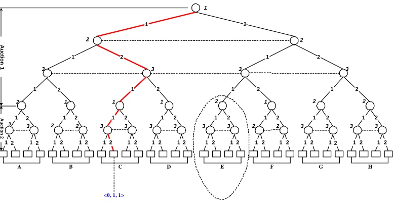
This game tree represents a 3-player -2-item sequential auction. This tree has 5 levels starting from the root node. Each node is labeled with a number, which represents the decision maker at that node. For example, the root node is labeled with 1, which means it’s player 1’s turn to make a decision. The first three levels represent the first auction with 3 players and are labeled Auction 1. The first level represents player 1’s choices; the 2 branches stemming from the root node means there are 2 bidding choices for player 1. The numbers on the branches are the amount player 1 can bid (To keep the figure manageable, all players can bid only 1 or 2 in this auction). The second level includes two nodes. These are decision nodes of player 2. They are connected by a dotted line to indicate that they are in the same information set -- in a sealed-bid auction, player 2 doesn’t know the bid of player 1. The third level has four nodes to represent the decision nodes of player 3. The four nodes are in single information set because player 3 doesn’t know the bids of either player 1 or player 2 when he makes decision.

participants of this sub-game are players 2 and 3, because in Auction 1, the bids of the three players are respectively 2,1,1. Player 1 is the highest bidder and leaves Auction 1 satisfied.

The leaf nodes are represented by squares. To illustrate how the players’ utilities are computed, we label the payoffs for the tenth terminal state. Payoffs are represented by a sequence of numbers in angle brackets (blue). The utility vector illustrated is based on the assumption that each agent’s valuation for an item is 3. To get this utility vector, we have to analyze the bidding path to the terminal state. The path is indicated by thick red path starting from the root node. The bidding path tells us in Auction 1, player 2 is the highest bidder and pays $2. Thus, the utility he can get is the valuation of this item to him minus the price he paid for it, $3-$2 = $1. In Auction 2, player 3 wins an item and also gets a utility of 1. Thus at the terminal state, players 2 and 3 each get a utility of 1, while player 1 wins nothing and gets zero utility.

This game tree contains all possible bidding paths in this sequential auction. Let A = {a1, a2, … , an} represent the set of agents participating this game, let V(A) = {V(a1), V(a2), … , V(an)}, where V(ai) represents the bid option vector for agent i. Then we

identical structures if ΓA≡ΓB.

3.3 Opponents’

strategy

Although our agent has incomplete information about its opponents, we assume all the other opponents are rational players and have complete information of the game, which means they know the other opponents’ valuations, including ours. In addition, they suppose all other players are rational, so they can just solve the game model as a complete information game and play the optimal Nash Equilibrium strategy.

3.4 Objective

computation. The size of the overall game tree will expand exponentially when the “move by nature” is introduced, which makes it even harder to solve the game.

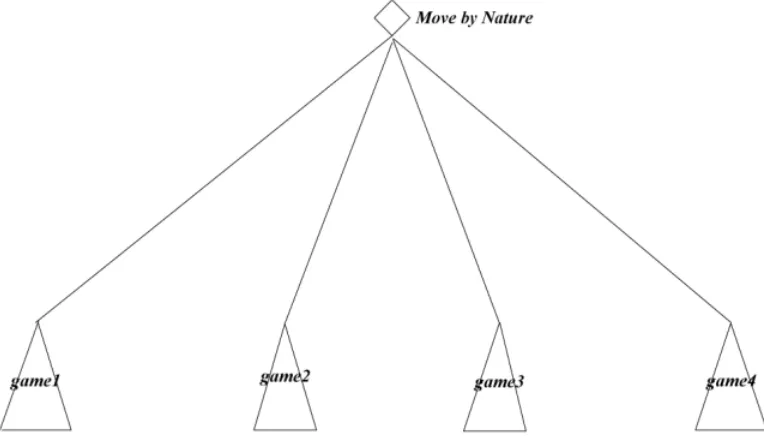
Let’s take the sequential game represented by Figure 3.1 as an example again. If there are only two possible valuations for each opponent, there will be 22 or 4 different games composed of the possible combinations of players’ valuations, as shown in Figure 3.2. The diamond node represents a move by nature. It’s branches are the four different states with different combinations of opponent’s valuations. For each state, there’s a game tree stemming from it, denoted by game1 to game4. These games share the same game tree structure with the game tree in Figure 3.1, but with different payoffs at the leaf nodes due to the different opponent’s valuations. If the number of possible valuations increases, the size of the overall game tree including the “move by nature” factor will expand exponentially. Therefore, the time it takes to solve a game will also increase exponentially.

will increase linearly with the Monte Carlo sample size. However, this is only an approximation.

Chapter 4

Implementation of Monte Carlo Sampling

4.1 Overview of Algorithm

Our goal is to construct a policy which tells our agent what action to take at every decision point. A data structure is needed to accumulate the policy. We choose a hash table to store the strategy vectors for each uniquely identifiable decision nodes for our agent. This hash table is initialized at the beginning of the algorithm.

The following steps are carried out repeatedly for every sample game:

1. Draw one sample opponents’ valuations from the continuous valuation distribution functions provided.

2. Construct a complete information game tree with GAMBIT using the valuations from step 1.

3. Solve the resulting complete information game and find an equilibrium strategy for our agent.

4. Update the bidding policy in the hash table according to the equilibrium strategy we get in step 3.

4.2 Constructing the game tree with GAMBIT

The construction of a game tree in GAMBIT proceeds in two steps: The first step is to build the game tree structure. We create the root node of the tree and then add decision nodes for each player. After each auction, the non-winners will participate in the following auction, if any. The winner leaves the game and enjoys his surplus.

The second step is to attach payoffs to every terminal node of the game tree. Every terminal node represents an end state of the sequential auction. These payoffs are essential when we compute the equilibrium strategies for each player. A Nash equilibrium is a strategy vector such that given the other player’s strategies, he can’t do better by deviating from his strategy. Much like a mutually beneficia l agreement between several nations, any unilateral deviation from this agreement will hurt the deviating nation itself.

sequential auction with 4 bid options as an example. The number of 4-player sub-game trees in this sequential game is 45, or 1024, but only 5 of them are unique -- the repeated sub-game structures appear very often. We need to store each of the possible sub-game structures only once. In this way, we need much less space to store the game tree structure and less time to solve this game tree.

4.3 Solving a game with GAMBIT (Backward induction and

intermediate caching techniques)

In GAMBIT, the approach to solv ing a game is to construct the game tree structure and then feed it into a game-solving module to get the result.

There are two reasons that we did not apply GAMBIT’s game-solving algorithm directly. First, the direct application of GAMBIT to solve a game calls for a complete game tree structure. But as we have explained in the previous section, we are unwilling to store the whole tree structure in memory. Instead, we store only the unique sub -game structures. The sub-trees A, E, G and H have identical tree structures, the sub-trees B, F and C, D also have the same structures in Figure 3.1.

game-solving algorithm directly due to the inefficiency. The GAMBIT game-solving algorithm uses the backward induction method, which is commonly used in AI and game theory. That is, it solves the game tree from bottom up. The problem with applying this algorithm directly to our model is that there are many identical sub-game structures that are solved repeatedly by GAMBIT. We improved the algorithm’s performance by caching the unique intermediate solutions to the sub-games (a dynamic programming approach) and use the lower level results to induce the upper level result. As an example, consider Figure 3.1. In GAMBIT’s algorithm, the eight sub -game trees have to be solved in order to solve the upper level game tree. In our improved algorithm, only three sub-game trees have to be solved.

The backward induction with caching algorithm works as follows:

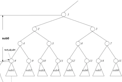
First step: We have the utilities each player expects in the lower level sub -games playing Nash equilibrium strategies. We add these utilities to the existing utilities of the leaf nodes of the higher level sub -games. For example, in figure 4.1 we will add the utilities players can get from sub1 to leaf node 8. The utilities each player expects in sub1, denoted by a utility vector <u1, u2, u3> should be added to the utilities

Second step: After we adjust the utilities of each leaf node of the higher level game tree sub0, we can solve this game tree with GAMBIT’s game-solving mo dule. In the same way, when we finish solving all the sub-game trees at this level, we can use these intermediate result to solve the next higher game until we reach the root of the game tree. The intermediate solutions in each level tell us exactly what strategy we should take at every decision node.

Figure 4.1 - Backward Induction During the Game-Solving

agent can find a solution at least ten times faster than using the default GAMBIT approach. This performance benefit increases with the size of the game tree. This feature greatly improves the scalability of the algorithm.

4.4 Monte Carlo based accumulation

After drawing a sample from the valuation distributions of each opponent, we build the corresponding game and solve it using the above-mentioned technique and store the equilibrium strategies of our agent. When doing this over many samples, we must aggregate the results. Given that the overall game tree has th e same structure over all samples (they only differ in the players ’ payoffs), it is easy to have a probability vector for each of our agent’s decision nodes, and accumulate the equilibrium strategies according to the position of the decision node in the game tree (Note: we only care about our agent’s decision nodes along the equilibrium strategy path. If the joint equilibrium strategy is a pure strategy, then this strategy path is a single path from the root node to the leaf node. If, however, it’s a mixed strategy, then the path will have some branches). For example, Let P = {p1, p2, p3, …pk} represents the set of

our agent’s decision nodes in the game tree, the value piuniquely identifies a position

of our agent’s decision node in the game tree structure, so there are a total of k

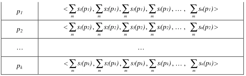
our agent has n bid options throughout the game. We can prepare a strategy vector

<s1(pi), s2(pi), s3(pi), sj(pi), … , sn(pi)>, when sj(pi) represents the probability of

choosing bid option j at position pi of the game tree. If we have m sample games, we

can accumulate the m strategies of our agent at position pi in these m different games

as < s(pi) m

1

∑

2

∑

3

∑

i

∑

n

∑

bidding path includes position pi, we will accumulate our agent’s equilibrium

strategy at this node, otherwise, the problem instance will have no effect on the node in question.

We could use a hash table to store all the strategy vectors as Table 4.1 -- one table item for one decision node of the game tree. When the size of the underlying game tree becomes large (more than a billion nodes), even the hard disk cannot accommodate such a large table. We develop a solution to tally all these strategy vectors, so that the information we need to store is much less.

Table 4.1 - Hash Table Used To Accumulate the Strategy Vectors According to a Decision Node’s Position In the Game Tree

p1 < s(p1)

m 1

∑

m 2

∑

m 3

∑

m i

∑

m n

∑

p2 < s(p2)

m 1

∑

m 2

∑

m 3

∑

m i

∑

m n

∑

… …

pk < s(pk)

m 1

∑

2

∑

3

∑

i

∑

n

Once again, we take advantage of the similarity between sub-games.

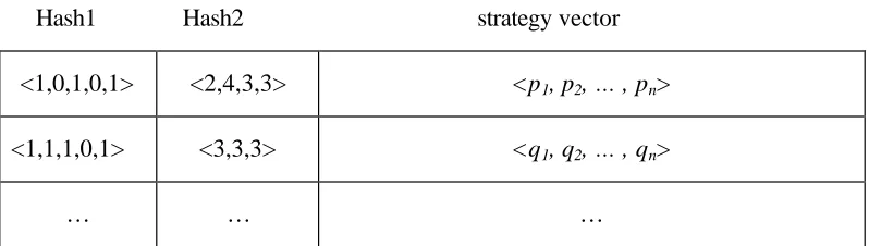
Table 4.2 – Hash Table Used To Implement History-Based Accumulation of Decision Node’s Strategy Vectors

Hash1 Hash2 strategy vector <1,0,1,0,1> <2,4,3,3> <p1, p2, … , pn>

<1,1,1,0,1> <3,3,3> <q1, q2, … , qn>

… … …

Based on this observation, we further distinguish the decision nodes according to the opponents’ actions in the previous auctions. Let A be the set of agents, and htbe the

bidding path before the t th round of auction. A(ht) represents the set of remaining

agents after the bidding path ht is followed. B(ht) represents the bids of the agents in A(ht) on path ht. We will treat two decision nodes as equivalent nodes and accumulate

their strategy vectors if and only if the sub-games stemming from them satisfy the conditions: B(ht) = B

^

(ht) and A(ht)= A

^

(ht). For example, in Figure 3.1, the nodes

that sub-trees B and F stem from are two equivalent nodes because they have identical tree structure and the only remaining opponent (player 2) bid the same ($1) in the previous auction.

evalu ate a decision node, we can check the corresponding hash table item to find the derived policy.

The hash value of this table is consisted of two parts: The first part is a value that uniquely identifies different sub -game structures. In Table 4.2, we use a vector to represent which players participate in a sub-game. For a 5-player sequential game, we use a 5-tuple vector <b1, b2, b3, b4, b5>. If player i participates in this sub-game, the ith bit will be set to 1, otherwise the bit will be set to 0. For ex ample, sub -games with players 1, 3 and 5 are represented by <1, 0, 1, 0, 1>, as in the first row of Table 4.2. The vector in the second row <1, 1, 1, 0, 1> represents a sub-game with four players: players 1, 2, 3 and 5. We use the corresponding binary number represented by this bitmap as the first part of the hash value.

the two previous auctions and player 5 bid $4 and $3. This is represented by the vector <2,4,3,3> in Table 4.2. The second row of Table 4.2 is a sub-game with 4 players left. Therefore, only one auction was held before this one. We need to model the other three opponents’ actions in previous auction. If they all bid 3 in this auction, the vector will be <3,3,3> , as in Table 4.2. We convert this into a uniquely identifiable value.

Combining these 2 values, we can get a hash value that can uniquely identify a decision node with the specific sub-game structure and opponent’s past bid behavior history. We then accumulate equilibrium strategies for nodes that are equivalent under this classification. This solution proves to save a lot of space; we need only several thousand rows in the hash table to accumulate a game tree with more than 1 billion decision nodes.

4.5 The factors that have to be weighted in the process of

accumulating

taken into consideration during the accumulation.

a. The probability of reaching this decision node

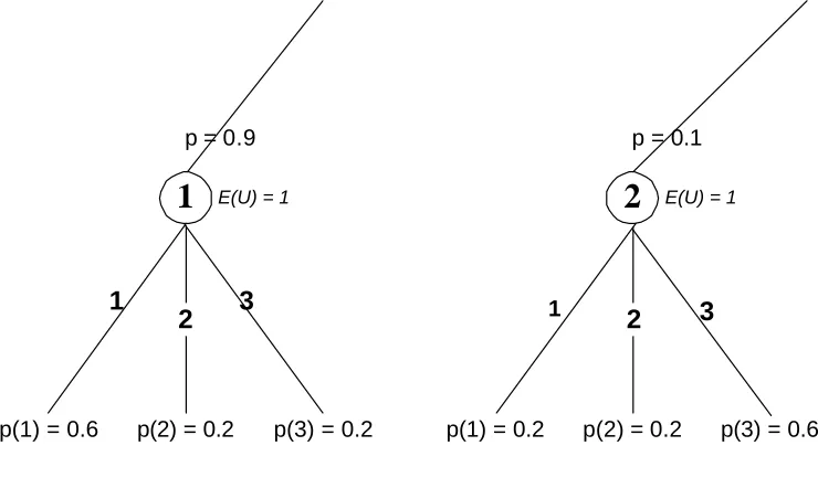
In figure 4.2, suppose decision node 1 and 2 are two equivalent nodes and are on the equilibrium paths in the same or different sample games. We should accumulate their strategy vectors into the same policy. The p value on the nodes represents the probability of reaching the node. The E(U) number represents the expected utilitiy of our agent when playing from the node. The numbers on the branches stemming from the nodes identify the bid options available our agent. p(i) represents the probability of choosing option i in the mixed strategy equilibrium.

2

1

2

2

3

1

3

p(1) = 0.6 p(2) = 0.2 p(3) = 0.2 p(1) = 0.2 p(2) = 0.2 p(3) = 0.6

p = 0.9 p = 0.1

E(U) = 1 E(U) = 1

Figure 4.2 – Two Equivalent Nodes

the p=0.9 and p=0.1 on the decision nodes when we accumulate the strategy vector <0.6,0.2,0,2> and <0.2,0.2,0.6>. According to the strategy vector of node 1, the mixed strategy favors bidding 1, but the strategy vector of node2 (<0.2, 0.2, 0.6>), the mixed strategy favors bidding 3. We certainly should add more weight to node 1’s strategy vector because we are more likely to reach node 1 than reach node 2, so the final accumulated strategy should be inclined toward node 1’s strategy. Thus, if we play more closely to node 1’s strategy vector, we will have a better chance of playing an equilibrium strategy.

b. The expected utility of the decision player at the decision node.

In Figure 4.2, we also need to consider the expected utility of decision player at these two nodes. The decision player at node 1 gets a larger utility than the player at node 2. So we should add more weight to node 1’s strategy vector because we are likely to get higher utility if we play in this way.

Generally, let S to be the set of sample games. We use T = {1, 2, 3, … ,t} to represent the set of equivalent decision nodes to be accumulated, and Π(t) represents the set of paths passing node t. Then Π(T) represents the set of all the possible paths that pass one of the equivalent nodes in the set T. Let Q(S) represents the set of all the possible equilibrium paths of the sample games in set S, and Ωt = Q(S) ∩Π(t) represents all

the equilibrium paths that pass an equivalent node in the set T. Let ωt∈Ωt to be one

of the paths within Ωt, p(ωt) represent the probabilities of reaching the equivalent

node t in the path, and u(ωt) represent our agent’s expected utility for the sub-game

from t. Let B = {b1, b2,…, bn} represent the set of possible actions our agent can take, Pr(ωt, bi) rep resents the probability of taking action bi in the equilibrium strategy at

equivalent node t on ωt. Then we accumulate these vectors:

<

∑

t)u( )Pr( ,b)

p(

ω ω ω ω ,

∑

2 t t

t)u( )Pr( ,b)

p(

ω ω ω ω ,...,

∑

n t t

t)u( )Pr( ,b )

p(

ω ω ω ω >

for every equivalent node t∈T.

4.6 How to use the heuristic strategy

come to a decision node that we need to make a decision for, we first compute a hash value according to the sub-game tree structure and the opponents’ bid history behavior and then use this value to lookup the policy decision. If a policy has been recorded for this node, we can use it. Otherwise, it means we did not record an equilibrium strategy path through this node in the sampling steps. In such case, we will try to find a similar decision node and adopt its strategy. When opponents have identical distributions for valuations, we consider a node similar if it has a d ifferent sub-game structure but with the same opponents’ history behavior. For example, node A with a sub-game tree of players 1, 2 and 4 and node B with a sub-game tree of players 1, 3 and 4 have different sub-game structures. If their opponents’ history behaviors are isomorphic , (Assuming player 1 is our agent), then we can say node A and node B are similar. In our simulations, we were able to find a strategy for most of the decision nodes in this way, if the similarity lookup failed, we randomly picked one choice or assigned equal probability to each choice.

4.7 Related work

n-bidder auction (k<n), an equilibrium point is reached when the bidders with the k

highest valuations are certain to receive items [9]. However, this strategy doesn’t ensure Nash equilibrium, that is, a bidder might be interested in deviating from this strategy seeking higher utility with other bidders ’ strategies fixed. So this might not be a feasible choice for self-interest bidders in the real world auctions. In our model, the agent attempts to “learn” a heuristic equilibrium strategy, which is an approximation of Nash equilibrium strategy that can ensure the mutual benefits of the participants.

Demange et al. develops a multi-item auction model, which is similar to our sequential auction model. Bidders are also interested in at most one item, but the difference is the bidders can only send a price vector to the au ctioneer once at the beginning of the auction, indicating how much he would like to pay for each of the items. So the bidders’ strategy in this model is fixed. They do not have a chance to observe other opponents’ actions in the auction and adjust their bidding strategy accordingly [10]. In our model, however, our agent will get more information about other bidders ’ strategies as the auction progresses. The decision we make will be based on those information.

dynamic programming model for agents to compute their bidding policies based on a prediction of the price distributions. They also describe how these distributions are reinforced iteratively in a learning model and converge to an optimal bidding behavior.

There are several conspicuous differences between our model and Boutilier’s:

First, our auction model is a single-item sequential auction, which means every player is interested in only one item. Whenever he wins one item, he will not participate in the following auctions. We make this assumption just to reduce the complexity of computation in this first investigation. We can relax this to two-item or more, but it will make the corresponding game tree structure more complex and take more time to solve. In contrast, Boutilier’s model assumes that the agent wants multiple items.

Third, due to the complementarities and substitutability of the goods in Boutilier’s sequential auction model, it’s impossible to get the exact value of a single item sold in the auction and make decisions based on that. This is one justification for using a dynamic programming approach to compute a bidding policy by which its bid for any item is conditioned on the outcome of events earlier in the round [1]. In our model, however, we take a different approach. We model our opponents individually and train our agent through fictitious play. Our agent will get experienced before it participates in the real auctions.

policy itself, we think it more reasonable to compare the expected payoff we can get from playing a Monte Carlo generated heuristic strategy with the expected payoff we can get from playing the optimal equilibrium strategy and see how close these two numbers are. As long as the expected payoff we can get from our Monte Carlo heuristic strategy is close enough to the optimal result, it will suggest that this might be a possible heuristic solution to this type of problems.

Howard James Bampton presents a Monte Carlo Heuristic to solve the Bridge in his thesis Solving the Imperfect Information Game using the Monte Carlo Heuristic [11]. Our works differs from his in two aspects:

First, he used the Monte Carlo method on the imperfect information game, but we go one step further, extending the application of Monte Carlo simulation to games with incomplete information.

we need to store the accumulated chance-minimax values of different alternatives for each of them. We develop a new way to classify the sampling data by the history behavior of the players. This method sharply reduces the data we need to store and makes it possible to solve larger-sized games.

Hon-Snir et al., propose an iterative learning approach to solve repeated first-price auctions in their paper, they develop a repeated auction model in which the agents learn the equilibrium strategy for a one-shot auction after many rounds of the repeated auction.

Their approach differs from ours in two aspects:

First, the performance of the strategies they use in these previous auctions is unknown. In contrast, our agent develops a strategy in all the sub-auctions of a sequential auction by fictitious play, and we ensure the overall performance of our agent in this sequential auction is acceptable.

Chapter 5

Experiment Data and Analysis

In our experimental simulation, we use a 5-player, 4-item sequential auction with four bid options. We compared the payoffs we can achieve using a Nash equilibrium strategy, our heuristic strategy and a myopic strategy in identical games. We also measured the social welfare of the allocation achieved with different combinations of strategies and compared them with the maximal social welfare. We ran Monte Carlo simulations with different samp le sizes to study the effect of sample size on performance. We are also interested in the relationship between the number of auctions and the performance of our Monte Carlo simulation agent. Also, we are interested in other distributions of opponent valuations.

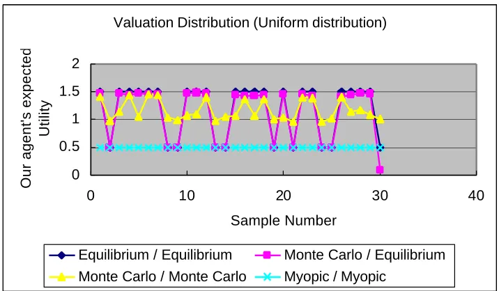
Figure 5.1 shows a comparison of the performance of our agent when it plays various strategies against different types of opponents.

Monte Carlo / Equilibrium – shows the performance of our agent using the heuristic strategy when playing against opponents playing the Nash equilibrium strategy.

Monte Carlo / Monte Carlo – all of the agents use the heuristic strategies generated by Monte Carlo simulation.

Myopic / Myopic – represents the case where all agents use a simple myopic strategy. The myopic strategy is to play the equilibrium strategy for each auction individually [8]. The optimality of the myopic strategy depends upon the assumption that the opponents’ valuations of the goods are uniformly distributed.

Valuation Distribution (Uniform distribution)

0 0.5 1 1.5 2

0 10 20 30 40

Sample Number

Our agent's expected

Utility

Equilibrium / Equilibrium Monte Carlo / Equilibrium

Monte Carlo / Monte Carlo Myopic / Myopic

In all of the simulations, our agent’s valuation remains in the middle of the valuation interval, while other opponents’ valuations will vary depending on different valuation distribution functions. Figure 5.1(a) shows our agent’s utilities in 30 problem instances where the other opponents’ valuations are drawn from a uniform distribution. In each problem instances we tested four combinations of strategies as explained above.

The experimental results show that our Monte Carlo sampling strategy performs better than the myopic strategy and quite close to the optimal equilibrium strategy. On average, the heuristic strategy performs better against opponents also playing the heuristic strategy than against opponents playing Nash equilibrium strategies. This result suggests that the Monte Carlo sampling strategy performs better when played against less informed opponents than against well-informed opponents.

Valuation Distribution (Left-skewed Beta distribution)

0 0.5 1 1.5 2

0 5 10 15 20 25 30 35 Sample Number

Our agent's expected

Utility

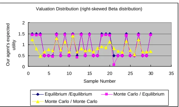
Valuation Distribution (right-skewed Beta distribution)

0 0.5 1 1.5 2

0 5 10 15 20 25 30 35

Sample Number

Our agent's expected

utility

Equilibrium /Equilibrium Monte Carlo / Equilibrium Monte Carlo / Monte Carlo

Figure 5.1(c) - Our Agent’s Expected Utility With Right-Skewed Beta Distributed Opponents’ Valuations

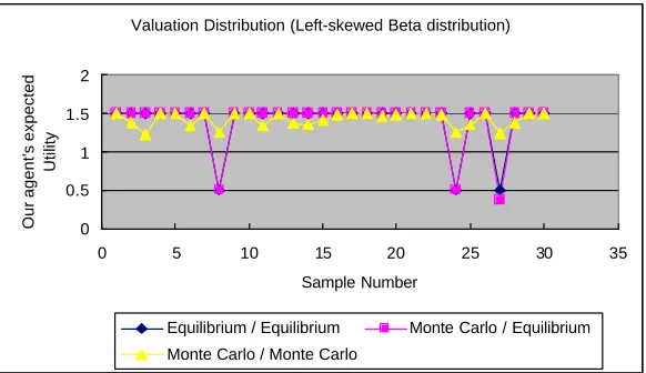
Figure 5.1(b) and (c) illustrate the corresponding results when opponents’ valuations are drawn from two non-uniform distributions.

valuations distribution and worse with right-skewed Beta distributed opponents’ valuation distribution. This corresponds to our expectation that with left-skewed Beta valuation distribution, out agent is more likely to be among the highest valuations and thus has a better chance of winning at a lower price and thus enjoy a higher utility.

We were also curious about the effect of the game theoretic behavior on the social welfare of the thirty sampled games. Figure5.2 illustrates the social welfare (all bidders ’ surplus plus the seller’s revenue) of this sequential auction. The diamond represents the maximal social utility of the game.

5-player-4item sequential auction (Uniform Valuation Distribution)

0 2 4 6 8 10 12 14 16

0 5 10 15 20 25 30 35

Sample Number

Social Utility

Optimal Equilibrium / Equilibrium Monte Carlo / Equilibrium Monte Carlo / Monte Carlo Myopic / Myopic

Figure 5.2 – Social Utility Comparison With Uniformly Distributed Valuations

allocation. The heuristic strategy will result in an allocation very close to the perfect one. The myopic strategy performs better than our heuristic strategy because it ensures the best allocation in each individual auction, which will definitely result in an optimal allocation for the whole game.

5-player-4item sequential auction

0. 95 0. 955 0. 96 0. 965 0. 97

0 50 100 150 200 250

Sample Size

Utility Ratio

Figure 5.3 – Our Agent’s Utility Ratio With Different Monte Carlo Sample Size

strategy.

Chapter 6

Conclusions and future work

During the course of the research embodied in this thesis, we developed a number of interesting insights and also found many avenues for additional work.

always ensures optimal allocation but generates quite poor returns for the agent.

Bibliography

[1] Craig Boutilier, Moises Goldszmidt and Bikash Sabata. Sequential Auctions for the Allocation of Resources with Complementarities, 16th International Joint Conference on Artificial Intelligence (IJCAI-99), Stockholm, August, 1999, pages 527-534.

[2] Ian Frank, David Basin, Hitoshi Matsubara. Monte-Carlo Sampling in games with imperfect information: Empirical Investigation and Analysis, Proceeding of the

Game Tree Search Workshop, 1997, http://citeseer.nj.nec.com/153153.htm l.

[3] Gambit Toolset homepage: http://www.hss.caltech.edu/gambit/.

[4] Graham, Romp. Game theory: introduction and applications, Oxford University Press, pages 8-12, 1997.

[5] Daphne Koller, Avi Pfeffer. Representations and Solutions for Game-Theoretic Problems, Artificial Intelligence 94(1), pages 167-215, July,1997.

[7] Shlomit Hon-Snir, Dov Monderer, Aner Sela. A Learning Approach To Auctions,

Journal of Economic Theory, 82, pages 65-88, 1998.

[8] R. Preston McAfee, John Mcmillan. Auctions and Bidding, Journal of Economic Literature, Vol. 25, pages 699-738, June, 1987.

[9] Robert J. Weber. Multiple-Object Auctions, in Auctions, Bidding, Contracting (R. Engelbrecht-Wiggans, M. Shubic, and J. Stark, Eds), pages 165-191, New York Univ. Press, New York, 1983.

[10] Gabrielle Demange, David Gale, Marilda Sotomayor. Multi-Item Auctions,

Journal of Political Economy, vol. 94, no. 4, pages 863-872, 1986.