Examine generalized lambda distribution fitting performance:
An application to extreme share return in Malaysia
Muhammad Fadhil Marsani
*, Ani Shabri and Nur Amalina Mat Jan
Department of Mathematical Science, Faculty of Science, Universiti Teknologi Malaysia, 81310 UTM Johor Bahru, Johor, Malaysia
* Corresponding author: [email protected]
Article history
Received 18 February 2017 Accepted 4 July 2017
Abstract
Understand the extreme volatility in the market is important for the investor to make a correct prediction. This paper evaluated the performance of generalized lambda distribution (GLD) by comparing with the popular probability distribution namely generalized extreme value (GEV), generalized logistic (GLO), generalized pareto (GPA), and pearson (PE3) using Kuala Lumpur composite index (KLCI) stock return data. The parameter for each distribution estimated using the L-moment method. Based on k-sample Anderson darling goodness of fit test, GLD performs well in weekly maximum and minimum period. Evidence for preferring GLD as an alternative to extreme value theory distribution also described.
Keywords: extreme share returns, Kuala Lumpur Composite Index (KLCI), L-moment, risk management, value at risk (VaR)
© 2017 Penerbit UTM Press. All rights reserved
INTRODUCTION
Market risk defined as the chance of loss or lower financial return from the share market. Investors tend to manage market risk actively because they want profitable returns. However, this volatility in the stock market is difficult to guess and may be influenced by an economic update (Chen, et al. 1986). For this, it is important for them to understand extreme volatility in the market to make a correct prediction. For that having proper probability distribution can produce an accurate estimate and improves risk management. In modeling stock returns, distribution assumption used is essential to create a good approximation. Risk measurement tools such as Value at Risk (VaR) and Expected shortfall (ES) estimate losses based on the quantile negative returns seen more efficient if the assumption used for distribution is correct. Study on the importance of the assumptions used for VaR distribution by Danielsson, et al. (1998) stated that the distribution of inappropriate assumptions produce inaccurate estimates and eventually carries the loss risk to investors.
Initially, stock returns typically are assumed distributed in a normal family. However, this assumption is no longer relevant because the available properties of the distribution of extreme stock returns in contrast to the normal distribution (NOR) which is fat-tailed (Fama 1965; Gray and French 1990; Peiró 1994; McDonald and Xu 1995; Theodossiou 1998; Harris and Küçüközmen 2001). Starting from the middle of the 1996 modeling extreme stock returns directed to extreme values theory EVT method (Longin 1996; Broussard and Booth 1998; Embrechts, et al., 1999; Longin 2000; Carvalhal and Mendes, 2003; Jondeau and Rockinger 2003). GEV distribution that can represent the extreme limit parameter equation of three distribution Fréchet, Gumbel, and Weibull used as a basis for an estimation of extreme events. They estimate VaR by applying extreme value theory EVT to model the tail of the distribution (Danielsson and de Vries, 1997; McNeil 1998; Longin 2000; McNeil and Frey 2000). Recently, many studies
highlighting generalized logistic (GLO) distribution is the best compared GEV in explaining volatility extreme stock returns, see (Gettinby, et al., 2004; Tolikas and Brown 2006; Tolikas 2008; Tolikas and Gettinby 2009; Tolikas 2014). Hussain and Li (2015) take part by analyzing stock returns data in China found that the GLO distribution fit extreme minimum returns very well while GEV distribution performs for extreme maximum returns. Among the studies that model extreme stock returns using Kuala Lumpur composite index (KLCI) data series is Hasan, et al. (2012) focus only on GEV distribution. Zin, et al. (2014) analyzed several distributions namely gumbel, generalized extreme value (GEV), generalized logistic (GLO), generalized pareto (GPA), lognormal (GNO) and pearson (PE3) distributions and found that GPA and PE3 distribution are the best in explaining stock returns KLCI for the period of maximum weekly and monthly respectively. Tukey (1962) introduced GLD distribution which was later updated by Ramberg and Schmeiser (1974). This distribution was found to have an excellent flexibility to generate parameter estimation. Distribution GLD widely applied in various fields such as meteorology (Öztürk and Dale 1982), process control statistics (Pal, 2004; Fournier, et al., 2006), income population (Tarsitano 2004), and the exchange rate (Corlu and Meterelliyoz 2014 ). Ability to use GLD to analyze stock returns increasingly recognized by researchers see (Corrado 2001; Chalabi, et al., 2010; Corlu, et al. 2016).
Based on these work it has motivated us to concentrate on the GLD, GEV, GLO, GPA, and PE3 distribution where these distributions has demonstrated exceptionally viable in clarifying the extreme event in environmental studies. This study is an extension of the existing research with the addition of GLD. Analysis of extreme stock market return using GLD are still not comprehensive and should have more attention. GLD distribution performance compares with other popular distributions such as GLO, GEV, GPA, and PE3 distribution still unknown and we will discuss the gap that remains in the scientific literature in this study. The focus of this study was to assess the
performance of GLD in modeling the distribution of extreme stock returns KLCI by comparing it with GEV, GLO, GPA, and PE3 distribution. The first contribution of this study is we have examined GLD capabilities in explaining extreme stock return volatility that has been less noted. Second, we compared the performance of GLD with other traditional distribution in extreme stock return using several approach namely l-moment ratio diagrams (LRD), k-sample Anderson-Darling test (k-ad), and analysis of tail distribution.
Data
KLCI daily stock returns data for 22 years used starting from 1994 until 2016 from Yahoo Finance is calculated using this formula
1
ln( / )
t t t
R P P where Rt is return index at t period, Pt is the stock
price index in the term of t, while Pt1 is the stock price index at the
time of t1. Weekly data interval in this study determined every five days and sub-period data divided into five periods, and it is calculated every three years begin from 1996 until 2016.
Fig. 1 Daily KLCI price index.
Figure 1 shows the KLCI daily stock price movement covers the years 1994 to 2016. Clearly, price index collapse first in the year 1998 recorded the lowest score of 200 and seconds in the year 2009 bottom at 800 due to the Asian and world economic crisis. Starting from 1994 until 1997 the price index remains to fluctuate for the range 1400 to 800. Economic recovery phase takes place when the price index raises reaching up to 1000 in the year 2000, however, the price decline to 600 in middle of the year 2001. The stock index is seen moderately rising for the years 2001 to 2008 and 2009 to 2016.
Fig. 2 Daily KLCI log return.
Figure 2 showed the stock price returns for the years 1994 to 2016. The index returns stay constant fluctuate about 0.05 and -0.05 regardless of extreme volatility. During the economy crisis in the year of 1997 to 1999 and 2008 to 2010 display high volatility during that term. The evidence from a decline of prices index leads to the high volatility we can say that there is a significant relationship between price movement direction and return index volatility.
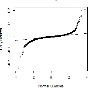
Figure 3 present normal QQ plot for daily log price index returns.
particularly in the upper and lower tail daily price return, indicating the data series are not normal and have a fat tail, we will further discuss this in section 3.4. Thus, it strengthens our claim that the data series should be estimated using GLD, GEV, GLO, GPA, and PE3 distribution.
Fig. 3 Normal QQ plot for daily log returns.
Table 1 is a summary statistics for daily and weekly maximum and minimum stock price return. Daily data series recorded the lowest return -24.153% and the highest 20.817%. Interestingly, both maximum and minimum return recorded in the year 1998 during economic crisis. The mean for daily return still positive 0.004% and the standard deviation is 1.389%. Skewness to measure distribution symmetriness is 0.426 expressing the tail inclined to the right. Significant kurtosis value of 53.503 proves that the distribution is fat-tailed and not normal. Focus on weekly series, negative mean values is recorded for minimum series return on the other hand positive mean value for the maximum series. The standard deviation value almost the same as maximum and minimum return recorded around 1.6% explain that the price returns volatility are not so noticeable between the maximum and minimum weekly series. High kurtosis for the weekly minimum return recorded at 73.343 gave the information that the distribution for this period is fat-tail. Note that the kurtosis value greater for minimum return series than maximum return series indicating a tail distribution is fatter for the minimum return case and extreme returns prone to occur on a minimum return series. Jarque-Bera test (JB) conducted to see the normality of the data dispersions. High JB value and significant p-value indicating that the data series for daily and weekly return did not follow a normal distribution. Here we notice that
JB value is getting smaller when the observations size decrease. Furthermore, JB for the weekly maximum and minimum return showed greater JB value in minimum returns indicating high abnormality return for minimum series than maximum.
Next section described the methodology including block maxima-minima (BMM), probability density function, estimation methods, and goodness of fit test.
Table 1 Summary statistics.
Daily Weekly
Minima Maxima
n 5556 1137 1137
min (%) -24.153 -24.153 -3.855
mean (%) 0.004 -1.093 1.134
max (%) 20.817 4.858 20.817
std. Deviation
(%) 1.389 1.685 1.604
variance (%) 0.019 0.028 0.026
skewness 0.426 -6.661 5.893
kurtosis 53.503 73.343 54.67
Jarque bera test 661620 183720 146890
METHODOLOGY
In this section, we explain the method used start with how the weekly minimum and maximum data series obtained from KLCI daily data series. Second, we described probability density function, quantile function and cumulative distribution function for each of the considered distribution. L-moment estimation method and goodness of fit test also presented.
Block maxima minima
Weekly return series in this study obtained through BMM where the maximum and minimum weekly series issued following a decided blocks of 5 days. This method can be expressed using mathematical equations as follows:
max( , ,..., ), max( , ,..., )
1 1 2 2 1 2 2
,..., max( , ,..., )
/ 1
x R R R x R R R
m m m m
x R R R
n m n m n m n
1, 2,..., n
R R R is daily price returns, n represent the total of the observed
sample while m is block length. According to Hussain and Li (2015), this method is merely adequate in modeling extreme volatility for a given period. Hence, in this study, we apply this approach for obtaining weekly maximum and minimum block return.
The distributions
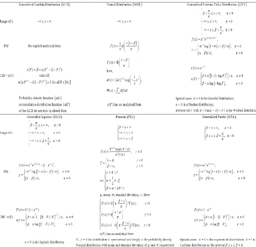
The probability density function, quantile function, and cumulative distribution function for each distribution that we consider in this study are as given in Table 2. Where x denotes the observed values of the random variable, f(x) is the probability density function,
x(F) is the quantile function, and F(x) is the cumulative distribution function. β is a location parameter represent mean value, α are scale parameters describe as standard deviation, κ and h are shape parameters define the tail fatness. Note that we also include normal distribution (NOR) information in Table 2 since we will use this distribution in the analysis of tail distribution.
The estimation method
We use L-moment method (LMOM) for parameter estimation instead of maximum likelihood estimation (MLE) since redundancy problem will appear in MLE method especially for models with many parameters. L-moment is linear combination of probability weighted moments (PWM). The concept of PWM described by Greenwood, et al. (1979) as:
10
where is the order of PWM
r th
r x F F dF r r
Hosking (1986) define L-moments in term of the PWMs as:
1 0
2 1 0
3 2 1 0
4 3 2 1 0
,
2 ,
6 6 ,
20 30 12 ,
L-moment ratios outline as:
2 2
1 2
, r, with 3
r r
where 1 is a location, is scale and dispersion (LCv), 3is the
measure of skewness and 4 is a measure of kurtosis (LCk). L-moment
is brief statistics for probability distribution and data samples.
The goodness of fit test
To examine the goodness of fit estimation, we apply L-moment ratio diagram (LRD) and K-sample Anderson-Darling (k-ad) Test.
L-moment ratio diagram
L-moment ratio diagram (LRD) introduced by Hosking 1990 explain the suitability of the data with the considered distribution. The L-skewness (3) and L-kurtosis (4) are plotted by x-axis and y-axis,
and each of the consider distribution curve is shown in LRD. Suitability of the data series with the distribution known based on the nearest 3
and 4 point with the distribution curve. LRD curve equation for each
distribution are as Table 3.
We can see that only L-moment ratio for NOR written in term of the point while GLD, GLO, GEV, GPA and PE3 distribution are written in term of equations forming the curve. Note that we obtain LRD equation for GLD by simplifying the equations derived by Karvanen and Nuutinen (2008), while GLO, GEV, GPA, and PE3 LRD equation we follow Hosking (1990).
K-sample Anderson darling test
K-sample Anderson-Darling (k-ad) test introduced by Scholz and Stephens (1987) is the generalization of the two-sample Anderson-Darling test. We take the advantages of mild parametric model assumptions on k-ad test to identify the best distribution performance in estimating the price return where this test could recognize the similarity and difference between two sample by taking into account the sensitivity at the tail. Another reason why we apply k-ad test instead of regular Anderson-Darling test is since GLD does not have closed form of PDF and CDF and it can only define in an inverse distribution function. A study conducted by Viglione, et al. (2007) compared the homogeneity tests for regional frequency analysis using k-ad test found that this test recommended for high skewness data. In this study, we proceed with k-ad test and the formula as the following:
2 1 0 ˆ ' '' 1 '
k i
k i
i
Fx x H x
AD n dH x
H x H x
where ni is the sample size of xi and H x'( ) denotes the empirical
distribution function of the pooled sample of all Fˆ ( )X i x , where 0 i k 1. k-ad test statistic signifies the difference between experimental and pooled samples value thus small k-ad test value means the differences are small and we can state that the distribution properly fitted the data.
Table 3 L-moment ratio diagram (LRD)curve equation.
GLD
2
3 3 3 3
3 4 4 4
3 3
5 1 5
0, ; 0, ;
5 5
GLO
2
4 1 53 / 6
GEV
2 3
4 3 3 3
4 5 6
3 3 3
0.10701 0.11090 0.84838 0.06669
0.00567 0.04208 0.03763
NOR 30, 40.1226
GPA 4 3
153
/ 53PE3
2 4
4 3 3
6 8
3 3
0.1224 0.3011 0.95812
0.57488 0.19383
Table 4 L-skewness and L-kurtosis price return.
Interval Period L-SKEWNESS (3) L-KURTOSIS (4)
Daily 1/4/1994 - 30/6/2016 -0.00834 0.330845
minimum
1/4/1994 - 30/6/2016 overall -0.37124 0.321025
1/7/1996 - 30/6/2000 1 -0.2754499 0.2685474
1/7/2000 - 30/6/2004 2 -0.2357384 0.2849451
1/7/2004 - 30/6/2008 3 -0.3261665 0.3333484
1/7/2008 - 30/6/2012 4 -0.390651 0.3546653
1/7/2002 - 30/6/2016 5 -0.24987193 0.19359507
maximum
1/4/1994 - 30/6/2016 overall 0.390715 0.338839
1/7/1996 - 30/6/2000 1 0.3111489 0.3027661
1/7/2000 - 30/6/2004 2 0.14187671 0.19149047
1/7/2004 - 30/6/2008 3 0.18651241 0.16699043
1/7/2008 - 30/6/2012 4 0.4582257 0.3999606
RESULTS AND DISCUSSION
Table 4 shows the L-moment ratio of L-skewness (3) and
L-kurtosis (4) for the daily and weekly minimum and maximum price
return. Weekly series for overall minimum and maximum period obtained from the year 1994-2016. The sub period divided every three years starting from 1996 to 2016 represent as 1,2,3,4, and 5. All of the weekly minimum interval returns shows negative L-skewness suggests that the tail of the distribution located on the left-hand side while maximum interval returns show a positive L-skewness implies that the tail of the distribution located on the right-hand side.
Figure 4 shows LRD in representing GLD, GLO, GEV, GPA, PE3, and NOR for daily and weekly maximum and minimum period. Note that, there are two curves of GLD, gld1 when 3 0 and gld2
when 4 0, intersection curves between gld1 and gld2 is the result
from the two different pairs values of 3 and 4 but matching the
L-skewness 3 and L-kurtosis 4. Note also overlap between distribution
curve gld1 and GPA due to both distributions have same properties. Overall, GLO curve distribution is the nearest to L-moment ratio point
3 and 4
for weekly maximum and minimum return excludes sub period-3 weekly maximum interval where this L-moment ratio point close to GEV distribution curve. Bear in mind, none of the LRD curves close to the daily L-moment ratio point. Also, LRD point for the NOR outcast all the data series. Hence, only weekly minimum and maximum interval considered in the further analysis and we omit NOR in next k-ad test.
Extreme minimum return
To determine the goodness of fit each of the distribution in describing price return volatility, we estimate overall and sub period weekly maximum and minimum return using GLD, GLO, GEV, GPA and PE3 distribution. Our focus is to identify the best distribution. Therefore we only showed the k-ad test result in Table 5 to examine the similarity between empirical and fitted data. The null hypothesis for k-ad test define as empirical and fitted data is homogenous and recall that lower k-ad value denotes the estimation getting sufficient. Referring Table 5, GLO and GLD distribution shows insignificant p-value at
5%
for all period indicating empirical and the fitted data are homogenous and the remaining distribution GEV, GPA, and PE3 displayed a significant p-value signifies empirical and fitted data come from different distribution.
Our result suggests that GLD is performing better than GLO in the overall weekly minimum return period with proof of lower k-ad test value 0.29709 for GLD less than 1.5648 for GLO. Meanwhile, for the sub-period return 1,2,3,4, and 5 recommend that the empirical and fitted data is not the same due to the significance of the p-value rejecting the hypothesis null suggest that GPA distribution is not suitable to estimate
minimum weekly return. Once again, GLD emerged as the best distribution for the weekly minimum returns with smaller k-ad test value compared with others distribution. In summary, GLD is excellent in explaining the extreme weekly minimum return event for the overall and the sub period. Next section we present the result for maximum weekly returns.
Extreme maximum return
Table 6 shows k-ad test result for maximum weekly price return series. Based on the overall period only GLD and GLO distribution have insignificant p-value means exist a similarity between empirical and the fitted price return. On the other hand, GEV, GPA, and PE3 have nonhomogenous empirical and the fitted data. Important to emphasize that the GLD perform way better than GLO with smaller k- ad test value 0.43455 compare to 2.0893. Move to the sub period, notice that GLD again give good estimation with the lowest k-ad test value for each of the subinterval compared with other distributions. Nice to highlight that this finding is opposed to the previous result in the last section LRD analysis in Figure 4 where we have found that GEV is the most suitable distribution in estimating weekly maximum return for the sub-period 3 as L-moment ratio close to the GEV curve distribution. This inconsistency between LRD and k-ad test may be due to the complexity of the GLD properties with two different pairs values of
3 and
4 byassuming either one to become zero lead to an unclear decision. Based on k-ad test we may conclude that GLD is the finest in estimating overall and sub-period for weekly maximum and minimum series return.
Analysis of tail distribution
Value at risk (VaR) operated at the end of the tail distribution could provide very useful potential losses information measured in term of probability. In this section, we consider analysis at the tail distribution on GLD, GLO, GEV, GPA, PE3, and NOR to investigate which of the distribution give better estimation at the tail. Note that, in this analysis again NOR considered as the comparing accuracy evidence at the upper and lower tail part for each of the series interval. Table 7 and 8 shows the probability of the weekly minimum and maximum return obtainable at the tail of the distribution according to eight different intervals for overall weekly minimum and maximum data series. Note that minimum interval located at the negative side or lower tail on the contrary maximum interval at the positive side or upper tail. Mean , and the standard deviation
, are calculated based on the overall weekly minimum and maximum data series respectively.In this analysis, we compare the actual probability return expressed as obs with the fitted probability return for GLD, GLO, GEV, GPA, PE3, and NOR. We consider NOR in this analysis so that we can verify the estimation ability at the upper and lower tail.
Table 5 Goodness of for minimum return.
Weekly GLD GLO GEV GPA PE3
Minimum k-ad p-value k-ad p-value k-ad p-value k-ad p-value k-ad p-value
overall 0.29709 0.94064 1.5648 0.16157 8.6819 5.00E-05 32.946 2.48E-18 9.6231 1.64E-05
1 0.23339 0.98068 0.23537 0.97982 0.98118 0.36692 3.7546 0.011311 0.84249 0.45162
2 0.10238 0.99998 0.44427 0.80551 1.7926 0.11925 5.3214 0.0019533 1.4629 0.18499
3 0.18644 0.99465 0.46426 0.78496 1.8955 0.10443 6.1613 0.0007632 1.8751 0.10719
4 0.32129 0.92361 0.46026 0.78909 2.0593 0.084805 7.4274 0.0002012 2.4099 0.055002
5 0.16117 0.99809 0.22042 0.98538 0.55296 0.69451 3.3841 0.017358 0.42431 0.82587
Table 6 Goodness of fit for maximum return.
Weekly GLD GLO GEV GPA PE3
Maximum k-ad p-value k-ad p-value k-ad p-value k-ad p-value k-ad p-value
overall 0.43455 0.81333 2.0893 0.082075 2.6212 0.042938 8.5916 5.51E-05 12.321 5.40E-07
1 0.17429 0.99676 0.25643 0.96939 0.40367 0.84757 1.2482 0.24918 1.1353 0.29287 2 0.26828 0.96192 0.29547 0.94375 0.38154 0.86863 1.5178 0.17168 0.46703 0.78209
3 0.20189 0.99118 0.31503 0.92872 0.27126 0.9601 1.0717 0.32123 0.38545 0.86481 4 0.13772 0.99952 0.64818 0.60432 0.75987 0.51132 2.0381 0.087102 3.9607 0.0090208
5 0.093867 0.99999 0.15814 0.99836 0.31556 0.92828 1.594 0.15493 0.51022 0.73763
From Table 7, we can say that both GLD and GLO performed well in capturing risk at the lower tail when the fitted and actual probability return display almost similar result. For example, the probability of the price return for actual data lies at the central interval
1 , 2
is 5.541% and it is close to GLD and GLO distribution estimation when both of the distribution has successfully capture 4.925% and 5.189% respectively. On the other hand, GEV, GPA, PE3, and NOR poorly estimate the tail by obtaining greater probability return than the actual percentage that is 7.124%, 13.017%, 7.212% and 7.564% respectively. Furthermore, all of the studied distribution excluding GPA and NOR provide nearly similar percentage at the lower tail interval specifically
6 , 7
,
7 , 8
and
8 , 9
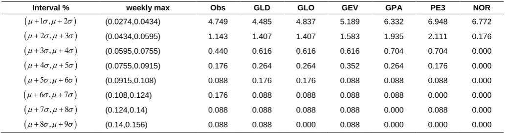
.Based on Table 8, weekly maximum case return shows a similar pattern with the previous minimum case return where GLD and GLO again give an outstanding result.This two distribution capture almost same percentage return with the observed data for each of the interval. Also, clearly we found that GEV, GPA, PE3, and NOR give bad prediction at the center tail distribution range by overestimating the price return. Moving to the upper tail interval particularly
6 , 7
,
7 , 8
and
8 , 9
we can see here GLD, GLO, GEV, GPA, and PE3 distribution give more or less same arrangement with the actual percentage. NOR failed to capture extreme maximum return at the upper part of the tail distribution due to zero percentage value starting from
3 , 4
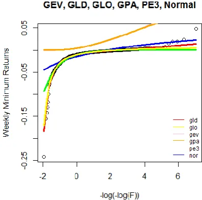
approaching high tail interval. Interestingly, GPA distribution shows better prediction at the upper tail for maximum return unlike at previous minimum return case. Consequently, based on the lower and upper tail analysis we may say that GLO and GLD give an adequate probability prediction especially at the central part of the distribution. Also, the assumption for minimum and maximum weekly return as NOR should be removed from the analysis since it miscarries the calculation.Figure 5 and 6 demonstrate plot distributions curve for weekly minimum and maximum price return to clarify upper and lower tail event. Note that we focus on the lower value for the minimum return and the upper value for maximum return.
From Figure 5 we found that GPA fitting curve distribution diverts from empirical data denotes GPA fail to predict minimum weekly price return adequately.Meanwhile, NOR and PE3 cannot predict extreme returns at the lower tail since the curve fails to reach smaller return. Although the distribution curve for the GLD, GLO, and GEV are overlapped between one to another indicating a very similar pattern for each of the distribution, GLD found to be more accurate in predicting minimum price return when the curve finds to be more closer to the
Fig. 5 Empirical against fitted distributions for weekly minimum returns series.
Table 7 Lower tail analysis for weekly minimum return.
Interval % weekly min Obs GLD GLO GEV GPA PE3 NOR
1 , 2
(-0.0262,-0.0416) 5.541 4.925 5.189 7.124 13.017 7.212 7.564
2 , 3
(-0.0416,-0.0571) 1.671 1.495 1.495 2.199 1.495 2.287 0.264
3 , 4
(-0.0571,-0.0725) 0.616 0.704 0.704 0.704 0.000 0.704 0.000
4 , 5
(-0.0725,-0.088) 0.176 0.264 0.264 0.264 0.000 0.176 0.000
5 , 6
(-0.088,-0.103) 0.088 0.176 0.176 0.088 0.000 0.088 0.000
6 , 7
(-0.103,-0.119) 0.088 0.176 0.088 0.000 0.000 0.000 0.000
7 , 8
(-0.119,-0.134) 0.088 0.000 0.088 0.088 0.000 0.088 0.000
8 , 9
(-0.134,-0.15) 0.088 0.088 0.000 0.000 0.000 0.000 0.000Table 8 Upper tail analysis for weekly maximum return.
Interval % weekly max Obs GLD GLO GEV GPA PE3 NOR
1 , 2
(0.0274,0.0434) 4.749 4.485 4.837 5.189 6.332 6.948 6.772
2 , 3
(0.0434,0.0595) 1.143 1.407 1.407 1.583 1.935 2.111 0.176
3 , 4
(0.0595,0.0755) 0.440 0.616 0.616 0.616 0.704 0.704 0.000
4 , 5
(0.0755,0.0915) 0.176 0.264 0.264 0.352 0.264 0.176 0.000
5 , 6
(0.0915,0.108) 0.088 0.176 0.176 0.088 0.088 0.088 0.000
6 , 7
(0.108,0.124) 0.176 0.088 0.088 0.088 0.088 0.000 0.000
7 , 8
(0.124,0.14) 0.088 0.088 0.088 0.088 0.000 0.088 0.000
8 , 9
(0.14,0.156) 0.088 0.088 0.000 0.088 0.000 0.000 0.000Next, distributions curve for weekly maximum return in Figure 6 show similar curve shape at the beginning of the index price return. However, the differences among the curve getting visible at the top of the return. A significant point to mention here is the distance between dispersions of the data with the fitted curve where the first closest fitted curve is GLD followed by GLO, PE3, GEV, GPA, and NOR. In summary for analysis of the upper and lower tail GLD happen to be the best distribution for both cases maximum and minimum weekly returns.
CONCLUSION
In this study, we investigate several distributions namely GLD, GLO, GEV, GPA, PE3 using Malaysia daily KLCI stock price data starting from 1994 to 2016. According to the analysis of LRD, k-ad test, and the Analysis of tail distribution we found GLD distribution gives better fitting performance compared to other distributions. GLD performance dominates both weekly maximum and minimum price return. Besides, GLO ranked as the second best distribution, and it is good to mention that the accomplishment is closely similar.
These findings give evidence for preferring GLD as best distribution in describing the extreme event in stock return since the performance is superior to other distribution which has been given less attention previously. The fitting accuracy provided in GLD can reduce the risks and provide benefits to investors. The GLD performance is unfolded not only for an overall weekly period but also apply to each sub-period returns. These findings also provide new knowledge in finance by improving the accuracy of estimation in extreme stock returns, particularly in Malaysia KLCI market share. This study might extend with the same methodology using others stock market data, for example, S&P500, Dow, Nasdaq, etc. to maximized the effectiveness of GLD in predicting stock return volatility.
ACKNOWLEDGEMENT
This work was financially supported by the Universiti Teknologi Malaysia under the Research University Grant and Ministry of Higher Education Malaysia
REFERENCES
Broussard, J. P., Booth, G. G. 1998. The behavior of extreme values in Germany's stock index futures: An application to intradaily margin setting.
European Journal of Operational Research. 104, 393-402.
Carvalhal, A., Mendes, B. V. 2003. Value-at-risk and extreme returns in Asian stock markets. International Journal of Business. 8(1), 1-24.
Chalabi, Y., Scott, D. J., Würtz, D. 2010. The generalized lambda distribution as an alternative to model financial returns. Eidgenössische Technische
Hochschule and University of Auckland, Zurich and Auckland. Retrieved
from Rmetrics Research Collection website: https://www.rmetrics.org/ sites/default/files/glambda_0.pdf.
Chen, N.-F., Roll, R., Ross, S. A. 1986. Economic forces and the stock market.
The Journal of Business. 59, 383-403.
Corlu, C. G., Meterelliyoz, M. 2014. Estimating the parameters of the generalized lambda distribution: Which method performs best?
Communications in Statistics-Simulation and Computation. 45(7),
2276-2296.
Corlu, C. G., Meterelliyoz, M., Tiniç, M. 2016. Empirical distributions of daily equity index returns: A comparison. Expert Systems with Applications. 54, 170-192.
Corrado, C. J. 2001. Option pricing based on the generalized lambda distribution. Journal of Futures Market, 21(3), 213-236.
Danielsson, J., De Vries, C. 1997. Beyond the sample: Extreme quantile and probability estimation. Tinbergen Institute Discussion Paper, 98-016/2. Danielsson, J., Hartmann, P., De Vries, C. 1998. The cost of conservatism:
Extreme returns, value-at-risk, and the basle ‘multiplication factor’. Risk.
11(1), 101-103.
Embrechts, P., Resnick, S. I., Samorodnitsky, G. 1999. Extreme value theory as a risk management tool. North American Actuarial Journal. 3, 30-41. Fama, E. F. 1965. The behavior of stock-market prices. The journal of Business.
38, 34-105.
Fournier, B., Rupin, N., Bigerelle, M., Najjar, D., Iost, A. 2006. Application of the generalized lambda distributions in a statistical process control methodology. Journal of Process Control. 16, 1087-1098.
Gettinby, G. D., Sinclair, C. D., Power, D. M., Brown, R. A. 2004. An analysis of the distribution of extreme share returns in the UK from 1975 to 2000.
Journal of Business Finance & Accounting. 31, 607-646.
Gray, J. B., French, D. W. 1990. Empirical comparisons of distributional models for stock index returns. Journal of Business Finance & Accounting. 17, 451-459.
several distributions expressable in inverse form. Water Resources
Research. 15, 1049-1054.
Harris, R. D. F., Küçüközmen, C. C. 2001. The empirical distribution of UK and US stock returns. Journal of Business Finance & Accounting. 28, 715-740. Hasan, H., Radi, N. F. A., Kassim, S., Baskoro, E. T., Suprijanto, D. 2012. Modeling the distribution of extreme share return in Malaysia using Generalized Extreme Value (GEV) distribution. In AIP Conference
Proceedings. 82-89.
Hosking, J. R. 1986. The theory of probability weighted moments, Research Report RC12210, IBM Research Division, Yorktown Heights, N.Y. Hosking, J. R. 1990. L-moments: analysis and estimation of distributions using
linear combinations of order statistics. Journal of the Royal Statistical
Society. Series B (Methodological). 52(1), 105-124.
Hussain, S. I., Li, S. 2015. Modeling the distribution of extreme returns in the Chinese stock market. Journal of International Financial Markets,
Institutions and Money. 34, 263-276.
Jondeau, E., Rockinger, M. 2003. Testing for differences in the tails of stock-market returns. Journal of Empirical Finance. 10, 559-581.
Karvanen, J., Nuutinen, A. 2008. Characterizing the generalized lambda distribution by L-moments. Computational Statistics & Data Analysis. 52, 1971-1983.
Longin, F. M. 1996. The asymptotic distribution of extreme stock market returns. Journal of Business. 69, 383-408.
Longin, F. M. 2000. From value at risk to stress testing: The extreme value approach. Journal of Banking & Finance. 24, 1097-1130.
Mcdonald, J. B., Xu, Y. J. 1995. A generalization of the beta distribution with applications. Journal of Econometrics. 66, 133-152.
Mcneil, A. J. 1998. Calculating quantile risk measures for financial return
series using extreme value theory. Retreived from ETH Zürich Research
Collection website: https://www.research-collection.ethz.ch/handle/ 20.500.11850/146132.
Mcneil, A. J., Frey, R. 2000. Estimation of tail-related risk measures for heteroscedastic financial time series: an extreme value approach. Journal
of Empirical Finance. 7, 271-300.
Öztürk, A., Dale, R. 1982. A study of fitting the generalized lambda distribution to solar radiation data. Journal of Applied Meteorology. 21, 995-1004. Pal, S. 2004. Evaluation of nonnormal process capability indices using
generalized lambda distribution. Quality Engineering. 17, 77-85. Peiró, A. 1994. The distribution of stock returns: International evidence. Applied
Financial Economics. 4, 431-439.
Ramberg, J. S., Schmeiser, B. W. 1974. An approximate method for generating asymmetric random variables. Communications of the ACM. 17, 78-82. Scholz, F. W., Stephens, M. A. 1987. K-sample Anderson–Darling tests. Journal
of the American Statistical Association. 82, 918-924.
Tarsitano, A. 2004. Fitting the generalized lambda distribution to income data.
In COMPSTAT’2004 Symposium. 1861-1867.
Theodossiou, P. 1998. Financial data and the skewed generalized t distribution.
Management Science. 44, 1650-1661.
Tolikas, K. 2014. Unexpected tails in risk measurement: Some international evidence. Journal of Banking & Finance. 40, 476-493.
Tolikas, K. 2008. Value-at-risk and extreme value distributions for financial returns. The Journal of Risk. 10, 31-77.
Tolikas, K., Brown, R. A. 2006. The distribution of the extreme daily share returns in the Athens stock exchange. European Journal of Finance. 12, 1-22.
Tolikas, K., Gettinby, G. D. 2009. Modelling the distribution of the extreme share returns in Singapore. Journal of Empirical Finance. 16, 254-263. Tukey, J. W. 1962. The future of data analysis. The Annals of Mathematical
Statistics. 33, 1-67.
Viglione, A., Laio, F., Claps, P. 2007. A comparison of homogeneity tests for regional frequency analysis. Water Resources Research. 43.
Zin, W. Z. W., Safari, M. a. M., Jaaman, S. H., Yie, W. L. S. 2014. Probability distribution of extreme share returns in Malaysia. In AIP Conference