Cooperative Distributed Energy Scheduling in Smart Grids

ABSTRACT

RAHBARI ASR, NAVID. Cooperative Distributed Energy Scheduling in Smart Grids. (Under the direction of Dr. Mo-Yuen Chow.)

Cooperative Distributed Energy Scheduling in Smart-Grids

by

Navid Rahbari-Asr

A dissertation submitted to the Graduate Faculty of North Carolina State University

in partial fulfillment of the requirements for the Degree of

Doctor of Philosophy

Electrical Engineering

Raleigh, North Carolina 2015

APPROVED BY:

______________________________ ______________________________ Mo-Yuen Chow Aranya Chakrabortty Chair of Advisory Committee

ii

DEDICATION

To My Parents

iii BIOGRAPHY

iv

ACKNOWLEDGMENTS

I would not be able to complete this dissertation without valuable guidance form people whose existence was a blessing for me during my PhD studies.

First of all, I am very grateful to Dr. Mo-Yuen Chow, my academic advisor, who was extremely supportive, encouraging, and patient toward my research. Not only he was an advisor, but a great mentor who spent lots of time with me to provide accurate feedback to stabilize, improve, and optimize the open loop response of my research.

Second, I want to thank my committee members, Dr. Yahya Fathi, Dr. Aryana Chakrabortty, and Dr. Huiyang Zhou whose questions, suggestions and critique during my oral exams, helped me to improve my research.

I also need to mention my colleagues in the ADAC group, who made the research environment extremely friendly and supportive and cooperated in different stages of my research. Specifically, I want to thank Dr. Unnati Ojha, Dr. Ziang Zhang, and Yuan Zhang who were my co-authors in multiple academic papers relating to my PhD research. I also thank Dr. Habiballah Rahimi Eichi, and Dr. Wente Zeng who provided valuable feedback during our weekly technical meetings regarding my research.

I am wordless to express my feelings toward my parents, Hamid Rahbari-Asr and Mahnaz Hashemi-Mehrabani. Their support, trust, and dedication were crucial in all stages of my life, especially during my PhD studies.

v

TABLE OF CONTENTS

LIST OF TABLES.. ... viii

LIST OF FIGURES.. ... ix

CHAPTER 1. INTRODUCTION ... 1

CHAPTER 2. Cooperative Distributed Demand Management for Community Charging of PHEV/PEVs Based on KKT Conditions and Consensus Networks ... 6

2.1 Introduction ... 7

2.2 Problem Formulation... 9

2.2.1 Objective Function ... 10

2.2.2 Relationship between SoC and charging power ... 10

2.2.3 Constraints ... 11

2.3 Distributed Charging Algorithm ... 14

2.3.1 KKT Conditions of Optimality... 14

2.3.2 Nonlinear Approximation of the Cost Function ... 14

2.3.3 Solution to the Optimization Problem ... 15

2.4 Distributed Implementation of the Algorithm ... 21

2.5 Simulation Results and Analysis ... 24

2.5.1 Case Study 1: Single–Step Optimization ... 26

2.5.2 Case Study2: Dynamic Optimization ... 29

2.5.3 Scalability Analysis ... 33

2.5.4 Sub-Optimality of the Algorithm due to Nonlinear Approximation: Benchmarking against nonlinear optimization solvers ... 36

vi

CHAPTER 3. Incremental Welfare Consensus Algorithm for Cooperative

Distributed Generation/Demand Response in Smart Grid ... 39

3.1 Introduction ... 39

3.2 Problem Formulation: Social Welfare Maximization in Energy Market 43 3.2.1 Welfare on the Demand Side ... 44

3.2.2 Welfare on the Generation Side ... 45

3.3 Incremental Welfare Consensus Algorithm ... 46

3.4 Numerical Results ... 60

3.4.1 IWC Algorithm on IEEE 39 Bus Test System ... 61

3.4.2 Monte Carlo Simulations for Scalability Analysis ... 63

3.5 Conclusion ... 64

CHAPTER 4. Distributed Real-Time Pricing Control for Large Scale Unidirectional V2G with Multiple Energy Suppliers ... 66

4.1 Introduction ... 67

4.2 Problem Formulation... 70

4.2.1 Objective Function ... 70

4.2.2 Constraints ... 76

4.3 Distributed Real Time Pricing for Charge/Generation Control ... 76

4.3.1 Simplifying the Objective Function ... 76

4.3.2 Augment the Objective Function with KKT Multipliers ... 77

4.3.3 Dual Decomposition ... 77

4.3.4 Distributed Observers to Estimate Global Information ... 78

4.3.5 Smart Transformers as Communication Nodes between Zones ... 79

4.4 Numerical Simulations ... 87

vii

CHAPTER 5. Asynchronous Incremental Welfare Consensus algorithm ... 93

5.1 Introduction ... 93

5.2 Incremental Welfare Consensus Algorithm ... 95

5.2.1 Distributed Estimation of Power Imbalance ... 96

5.3 Local Price Update ... 96

5.4 Power Regulation ... 97

5.5 Sensitivity of IWC to Synchronous Updates... 99

5.6 Asynchronous Incremental Welfare Consensus Algorithm ... 100

5.6.1 Communicating nodes ... 102

5.6.2 Non-communicating nodes ... 103

5.7 Numerical Results ... 103

5.8 Conclusion ... 106

CHAPTER 6. Consensus Based Distributed Scheduling for Cooperative Operation of Distributed Energy Resources and Storage Devices in Smart Grids ... 107

6.1 Introduction ... 107

6.2 Problem Formulation... 110

6.2.1 Objective function ... 110

6.2.2 Controllable Inputs ... 111

6.2.3 Uncontrollable Inputs ... 112

6.2.4 System States ... 112

6.2.5 Operational Cost ... 112

6.2.6 Constraints ... 113

6.3 Consensus based distributed iterative algorithm ... 114

viii

6.3.2 Distributed estimation of global information with consensus

networks ... 117

6.4 Numerical Simulations ... 128

6.4.1 Demonstrate the application of the algorithm ... 128

6.4.2 Robustness to communication link failures ... 132

6.4.3 Validate the convergence of the algorithm to global optimum using Monte Carlo simulations ... 134

6.5 Conclusion ... 137

CHAPTER 7. Conclusion ... 138

ix

LIST OF TABLES

Table 2-1: Cooperative Distributed PHEV/PEV Demand Management (CDPDM)

Algorithm ...23

Table 2-2: Information About the Vehicles in the 1st _{Case Study ...27}

Table 2-3: Information About the Vehicles in the 2nd Case Study ...30

Table 2-4: Monte Carlo Simulation Sampling Range ...34

Table 3-1: Generation and Demand Unit Cost/Utility Function Parameters Chosen for IEEE-39 Power Network ...61

Table 4-1. Dispatchable Unit Parameters Chosen for the Case Study ...89

Table 4-2. Generated/Consumed Power By Non-Dispatchable Units ...89

Table 5-1. Generation/Demand Units Parameters Chosen For Garver Network ...99

Table 6-1. Node Types in the Network ...130

x

LIST OF FIGURES

xi

xii

Figure 5-5. A typical communications scenario for AIWC algorithm running on the

Garver power network ...103

Figure 5-6. Evolution of a) generation/consumption powers, b) social welfare value, c) price and d) total generation/demand in AIWC algorithm ...104

Figure 5-7. Evolution of generation, demand and social welfare for AIWC algorithm under probability of asynchronous behavior for the pairwise updates a) p = 0.1, b) p = 0.2, c) p = 0.5 ...105

Figure 6-1. Structure of a microgrid with distributed controllers ...111

Figure 6-2. General structure for each distributed controller ...118

Figure 6-3. Five bus power network with multiple energy devices ...129

Figure 6-4. Input profiles for the case study ...130

Figure 6-5. Convergence of dual variable estimations (a) for all time steps at node 1, (b) at all nodes for time step 2, and (c) discharging rate decisions of DESDs for different time steps ...131

Figure 6-6. Resultant schedule of the proposed distributed scheduling approach and energy stored in each storage device ...132

Figure 6-7. Convergence of the objective value (blue line) to the global optimum (red line) ...133

Figure 6-8. Algorithm convergence with/without communication link failures in the 5 bus network ...134

xiii

1

CHAPTER 1. INTRODUCTION

The future power system would be an aggregation of distributed generation units, responsive demands, and storage units each equipped with controllable power electronics devices connected to each other through the communications network [1], [2]. This Cyber-Physical System (CPS) is called “Smart-Grid”, and as shown in Figure 1-1, is geographically distributed and consists of a multitude of heterogeneous devices.

Distinguishing characteristics and benefits of the smart grid according to the Energy Independence and Security Act of 2007 (EISA) and National Institute of Technology (NIST) include [3]:

1. Dynamic optimization of grid operations and resources with full cyber-security,

1 _{Picture from http://www.consumerenergyreport.com/smart-grid/}

2

2. Predictive maintenance and “self-healing” responses to system disturbances/changes,

3. Development and incorporation of demand response, demand-side resources, and energy-efficiency resources,

4. Deployment and integration of advanced electricity storage and peak-shaving technologies, including plug-in electric and hybrid electric vehicles, and thermal-storage air conditioning,

To reach these goals requires advanced control and optimization technologies. Managing the smart-grid, considering the number and variety of controllable devices necessitates a paradigm shift in traditional Energy Management Systems (EMSs), which are operated centrally through Supervisory, Control, and Data Acquisition (SCADA) systems [1], [4]. This paradigm shift needs to consider the local intelligence of the distributed devices, as well as their communications capability [5].

Self-organizing, distributed systems can provide useful solutions for developing scalable and robust algorithms for energy management in the smart gird. Many of the dynamic systems in the nature as shown in Figure 1-1 are composed of multiple smaller units which sense their environment locally, perform local computations, and coordinate with their neighbors to carry out complex tasks. Examples include ant colony [6], bird flock [7], vehicles in a transportation system, people in a social network, and biological cells inside our body. Distributed algorithms have been studied in several areas, such as social science, animal science [8], computer science [9], distributed estimation [10], [11], and distributed identification [12] .

3

system consisting of multiple distributed devices with local computational and communications capabilities.

This thesis presents the author’s work in developing distributed energy management and scheduling techniques for resources, demands, and storage devices in smart grids. Multiple fully distributed algorithms are developed each for solving a particular energy management/scheduling problem. Chapters 2 to 6 are each dedicated to explaining one algorithm. The organization of chapters are as follows:

Chapter 2 presents Cooperative Distributed Plug in Electric Vehicle Demand Management (CDPDM) algorithm for distributed demand side management of large scale Plug in Hybrid /Plug in Electric Vehicles (PHEV/PEV) charging considering limit on the total available power. The problem is to optimally allocate the available charging resources among multiple PHEV/PEVs integrated to the grid, based on their priority without employing any control center. In this structure the charging stations are capable of communicating with their local neighbors and can perform local computations.

(a) (b)

4

Chapter 3 addresses a more general problem: energy management for a smart grid populated with responsive demands and distributed generators using local communications and computational capabilities of distributed resources. The objective is to develop a distributed cooperative scheme such that the responsive demands and distributed generators can optimally change their consumption or generation level in real-time in response to the varying conditions of the grid (such as changes in the production level of renewables, increase in the nonresponsive demands, etc.). Incremental Welfare Consensus (IWC) algorithm is proposed to solve this problem.

Chapter 4 addresses the problem of managing PHEV/PEV charging considering multiple heterogeneous resources on the generation side. The problem considered in this chapter is different than the one in chapter 2. In chapter 2, we had only one limited source of energy, while in chapter 5, we consider multiple renewable and conventional energy resources each with different cost of providing the energy. Based on the framework of IWC algorithm, Distributed Real-Time Pricing for Charging and Generation Control (DRPCG) is proposed to solve this problem.

Chapter 5 proposes Asynchronous Incremental Welfare Consensus (AIWC) algorithm to relieve the synchronous update requirement from the IWC algorithm. The algorithm proposed in chapter 3, requires each device to update its states synchronously with all the other devices. Retaining synchronous behavior over thousands of devices in a geographically distributed system is not a realistic assumption. Therefore, this chapter extends the IWC algorithm into an asynchronous version obviating the necessity of synchronous updates.

5

(CODES) algorithm was proposed to schedule the charging/discharging of storage devices and generation of dispatchable units to minimize the defined cost index of the system. While all the problems considered in the previous chapters were single time step optimization problems, this chapter addresses a multi-time step optimization problem, because by introducing storage devices, energy decisions at different time steps are no longer independent of each other.

6

CHAPTER 2. COOPERATIVE DISTRIBUTED DEMAND MANAGEMENT FOR COMMUNITY CHARGING OF PHEV/PEVS BASED ON KKT CONDITIONS AND

CONSENSUS NETWORKS

Abstract:

7

2.1 Introduction

Technologies used to update utility electricity systems with computer-based automation and control through two-way communications structures constitute the core of the “smart grid” concept [13]. Enabling the transition to in Hybrid Electrical Vehicles (PHEVs) and Plug-in Electrical Vehicles (PEVs) is one of the anticipated benefits of the smart grid [3]. These vehicles provide many incentives for the transportation industry and the environment [14]. Large-scale integration of these vehicles has potential impacts and benefits for the grid. One of the apparent impacts is the increase of the peak demand [15] which can destabilize the grid if not managed properly. On the other hand, the PHEV/PEVs can benefit the grid by being treated as a flexible load through charge/discharge scheduling to shape the load profile [15], [16]. Moreover, on the customer side, the increased satisfaction from the charging process in terms of time and cost of charging as well as the State of Charge (SoC) of the vehicle when leaving the charging station, can improve the adoption rate of the electric vehicles. Therefore, employing efficient energy-management policies to control and optimize the charging process for electric vehicles is becoming a critical need for the future grid. The enabling technology is called Vehicle to Grid (V2G) technology [17]. In general, V2G technology is operated in large scale and involves optimization strategies with single or multiple objectives [18]. The process of optimal dispatch of PHEV/PEVs using the V2G technology is called “Smart-Charging” [19], [20]. The focus of this chapter is on a “Smart-Charging” method using unidirectional V2G technology.

8

the optimal power allocation for each unit and transmits it to the charging stations [21]–[24]. The centralized approach works well for small-scale problems with a small number of vehicles where each unit can send information to the central controller directly without congestion. However, as the number of PHEVs/PEVs increases and they spread over a wide zone, such as a large city, the centralized approach loses efficiency due to two main reasons: 1) the required communications and computational capacity of the control center grows as the dimension of the problem increases, 2) the system becomes fragile to single points of failure.

To solve the issues of centralized smart charging for large scale problems, research has started on decentralized PHEV/PEV demand control. In most of the proposed decentralized approaches in the literature, each charging station regulates its own power by responding to an external signal [25]–[30]. Therefore the computational burden is relieved from the control center. However, still a center/aggregator is required to send the coordinating/pricing signals. Specifically, in [25], low-voltage transformers coordinate with each other by communicating with a high-voltage transformer to reduce the imbalances; In [26]–[28] the utility sends a central price/event signal to all the charging stations to manage the aggregate charging load; In [29] the distributed units respond to changes in the price signal adjusted through a center and in [30] a hierarchical decentralized method is introduced in which central aggregator broadcasts update/average information back and forth to/from sub-aggregators and in some cases the global constraint to avoid overloads is violated.

In this chapter, we introduce a cooperative distributed optimal power-allocation algorithm to satisfy grid constraints and customer preferences for large-scale charging of PHEVs/PEVs.

9

has no central aggregator/coordinator unit. Consequently, single-node congestion is alleviated, and the system becomes more robust against single points of failures. Moreover, the computational and communications burden is divided among the distributed processors, so the proposed approach is scalable. Unlike approaches that are based on dual decomposition (e.g., [30]), in our algorithm prior to the convergence, the global constraint is never violated.

The idea of our algorithm is shown in Figure 2-1 . Related work is done in [31]. The current chapter explains the algorithm in theoretical details and studies its scalability and sub-optimality and compares it with centralized algorithms. Similar concepts are also used in our research group to optimally manage distributed energy resources on the generation side [32].

Organization of this chapter is as follows: Section II provides the problem statement. In section III, we propose our distributed consensus-based algorithm. Section IV presents the numerical analysis and results, and the concluding remarks are made in Section V.

2.2 Problem Formulation

The problem of PHEV/PEV community charge allocation can be formulated as an optimization problem consisting of an objective function and appropriate constraints.

10

2.2.1 Objective Function

Different factors, such as battery longevity [21], the amount of charge and the tightness of the deadline [22], the flattening of the overall load profile and reducing the load variance [33], and the cost of charging for vehicle owners [28], can be considered in defining the objective function for PHEV/PEV charge coordination.

Satisfaction of the PHEV/PEV users from the charging service is directly related to the State of Charge (SoC) of the vehicle, when leaving the charging station. Therefore, in this chapter, similar to [23], the objective function is defined as the weighted sum of the State of Charge (SoC) of the vehicles at the next time step:

( )

1

Max ( ) ( 1)

N

i i

P k i

J w k SoC k





_

where ( ) = [ ( )] ,.., is the vector of the power allocated to the vehicles, N is the total

number of vehicles, SoCi(k+1) is the SoC of the battery pack of the ith vehicle at the next iteration, and wi(k) is the priority weighting for the ith vehicle, as well as a nonnegative value. Depending on the desired performance, the weights can prioritize vehicles based on the remaining time of charge, remaining battery capacity to be charged, and/or the customer’s willingness to pay.

2.2.2 Relationship between SoC and charging power

11

complicated battery models can be considered in the optimization process, and this would be one of the future works of the authors. Considering the capacitance model, the equivalent capacitance of the ith battery, Ci, is then calculated as:





,max ,min

( ) ( )

i i i

i

i i

Q SoC SoC

C

V SoC V SoC

 

 , (2-2)

where Qi is the capacity of the ith battery in Coulombs and [ _, , _, ] is the operating range of the battery. The change in the charge of the battery at each time step, k, would be ∆ ( ) = ∆ ( ). So, we can write:

( 1) ( )

( 1) ( ) i i i i

i i

i

CV k CV k

SoC k SoC k

Q

 

   . (2-3)

The energy provided to the battery during each time step, ∆ , would be ∆ . Considering the efficiency of the charging to be , the energy stored in the battery would equal Δ . Applying conservation of energy,

2 2

1 1

( 1) ( )

2C V ki i  2C V ki i iP ti

(2-4) Substituting for

V k

(



1)

2 2 ( )

( 1) ( ) i ( ) ( ) i i

i i i i

i i

C P k t

SoC k SoC k V k V k

Q C



 _ 

   _   _

 

 

. (2-5)

2.2.3 Constraints

Constraints represent the physical limits:

2.2.3.1 Global constraint

There is a limit on the total amount of power that the utility can allocate for charging purposes,

12 1

( ) .

N

i total

i

P k P







2.2.3.2 Local constraint

Certain factors impose local bounds on the amount of allocated power for each unit. For instance, the maximum power output of the outlet (e.g., 4.6kW for a standard single-phase 230V outlet), level of charging (e.g., 1.33kW for level 1), the maximum tolerable charging current, , and the maximum allowable SoC, (SoCmax), to avoid overcharging. These constraints are mapped into one constraint for each unit:

,max

0P k_i( )P_i ( ) ,k  i 1,...,N ,

(2-7) where _, ( ) is the upper bound of the allocated power considering all the local limitations. As the Vehicle-to-Grid (V2G) capability is not considered here, the lower bound is set to zero, so the PHEV/PEVs should not be discharged.

2.2.3.3 Optimization Problem Structure

Substituting for

SoC k

(



1)

2 ( )

1 1 1

2 ( )

Max ( ) ( ) ( ) ( ) ( ) .

N N N

i i i

i i i i i

P k

i i i i i

C P k t

J w k SoC k V k w k V k

Q C



  











The first two summations in (2-8) are independent of the decision variables P k_i( ) and therefore can be eliminated from the objective function,

2 ( )

1

2 ( )

Max ( ) ( ) .

N

i i

i i

P k

i i

P k t

J w k V k

C







13

To simplify the notations we introduce ( ) = ( ) / 2 Δ / , and ( ) =

( ) /2 Δ and rephrase (2-9) as:

( )

1

Max ( ) ( ) ( ) .

N

i i i

P k i

J











Considering the constraints, the optimization problem in terms of the allocated charging powers can be expressed as:

( )

1 1

Min ( ) ( ) ( ) ( ) ( )

N N

i i i i i

P k

i i

J







 

 

_

_

subject to:

1

( ) ,

N

i total

i

P k P







,max

0P ki( )Pi ( ),k  i 1,...,N.

(2-11)

Remark 2-1:

14

2.3 Distributed Charging Algorithm

Our distributed charging algorithm is based on Karush-Kuhn-Tucker (KKT) conditions of optimality [23]:

2.3.1 KKT Conditions of Optimality

Consider the general optimization problem of the form:

Min ( ) subject to:

( ) 0, 1,..., ,

( ) 0, 1,..., .

i

j

J x

h x i n

g x j m

  

  

(2-12)

If x*is a solution of (2-12), then there are constants ( = 1, … , ) and ( = 1, … , ), called KKT multipliers [34], such that:

* * *

1 1

( ) ( ) ( ) 0 ,

n m

i i i i

i i

J x  h x  g x

 

 

_

_

* *

( ) 0 , 1,..., , ( ) 0 , 1,..., ,

i

i

h x i n

g x i m

  

   (2-14)

*

( ) 0 , 1,...,

ig xi i m

    , (2-15)

0, 1,...,

i i m

    . (2-16)

The conditions (2-13), (2-14), (2-15), and (2-16) are called KKT conditions and are necessary for optimality. When the objective function is convex and the constraints are affine (as in our case), the KKT conditions are sufficient for global optimality as well [34].

2.3.2 Nonlinear Approximation of the Cost Function

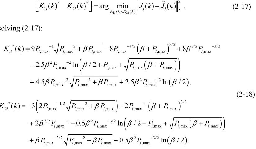
In order to simplify the optimization process, we approximate = ( ) + ( ) in (2-11) with = ( ) ( ) + and choose K1i(k) and K2i(k) to minimize the norm of the

15 1 2

2

* *

1 2 ₂

( ), ( )

( ) ( ) arg min ( ) ( )

i i

i i i i

K k K k

K k K k J k J k

   

   . (2-17)

By solving (2-17):

















3/2

* 1 2 3/2 3/2 3/ 2

1 ,max ,max ,max ,max ,max ,max 2 2

,max ,max ,max ,max

2 2 2 2

,max ,max ,max ,max

( ) 9 8 8

2.5 ln / 2

4.5 2.5 ln / 2 ,

i i i i i i i

i i i i

i i i i

K k P P P P P P

P P P P

P P P P

                           





















* 1/ 2 2 1

2 ,max ,max ,max ,max ,max 3/ 2 1 2 3/ 2

,max ,max ,max ,max ,max

3/ 2 2 2 3/ 2

,max ,max ,max ,max

( ) 3 2 2

2 0.5 ln / 2

0.5 ln / 2 .

i i i i i i

i i i i i

i i i i

K k P P P P P

P P P P P

P P P P

                             (2-18)

With this approximation, we can write the optimization problem as (2-19) where ( ) = ∗_{( ) ( ). Note that as} ∗_{( ) is a constant addition, it can be eliminated from the objective}

function.

' ( )

1

Min ( ) ( )

N

i i

P k

i

J





 



subject to:

,max 1

( ) , 0 ( ) ( ), 1,..., .

N

i total i i

i

P k P P k P k i N



    



(2-19)

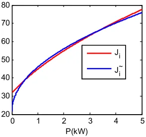
Figure 2-2 shows the curves of ( ) and ( ) for β = 1000, and Pi,max(k) = 5 kW. The effect of this approximation on the optimality of the solutions will be studied in section IV.

2.3.3 Solution to the Optimization Problem

16

*

( )

0, 1,...,

2 ( )

i

i i

i k

i N

P k



  

 

      , (2-20)

where λ is the KKT multiplier associated with the global inequality constraint and and for i=1,…, N are associated with the local constraints (one for each of the bounds).

If the local inequality constraints are strictly satisfied at the optimal point, based on (2-15), we would have = = 0. Applying this to (2-20), we get a positive value for , which indicates that ∑ ( ) = based on the condition (2-15). Solving for Pi(k)*:

2 *

2 1

( )

( ) , 1,...,

( )

i

i N total

j j

k

P k P i N

k

 





  





. _(2-21)

The value for Pi(k)* already satisfies the non-negativity constraint. This trait is the direct result of the approximation in section II.B. In order to guarantee that the upper bound limits are also satisfied, we set those values of ( )∗ that violate the local maximum bound to their maximum value and exclude their values from . Then, we use the same procedure in (2-21) to allocate the remaining power to the remaining vehicles. This procedure is written as Algorithm 2-1.

Figure 2-2: The actual objective function and the approximated objective function

0 1 2 3 4 5

20 30 40 50 60 70 80

17 Algorithm 2-1:

1. Set I = {1, 2, …, N} , n = 1 ,U1 = ∅ . 2. For all ∈ − , calculate P k_in( )** as:

2 ** ,max 2 ( ) ( )

( ) n

n

n i

i total j

j U j

j I U k

P k P P

k          _  _   





3. Set U1 = ∅. For all ∈ − , if P k_in( )**> Pi,max(k), update U1= U1 + {i}.

4. If U1 = ∅, go to step 5. Otherwise, set Un+1 = Un+ U1, n =n + 1, and Go to step 2. 5. Stop the algorithm. Set U = Un. The optimal powers are assigned as follows:

a. For all i I U,

2 * ,max 2 ( ) ( ) ( ) i

i total j

j U j

j I U k

P k P P

k          _  _   





b. For all iU , P k_i( )* P_i,max( )k .

These iterations are repeated until all vehicles receive a valid allocation of power. This method of allocating powers terminates in maximum of N iterations, and the final point satisfies the KKT conditions of optimality.

Theorem 2-1:

The final point * *

( ) i ( )

P k _{ }P k _ resulted from Algorithm 2-1, satisfies the KKT conditions of optimality for optimization problem in (2-19).

Proof:

The Lagrangian for (2-19) can be written as follows:





'

,max

1 1 1 1

( ) ( ) ( ) ( ) ( ) ( ).

N N N N

i i i total i i i i i

i i i i

L  k P k  P k P  P k P k P k

   

 

   _  _  

 

18

Let’s denote the final point resulted from Algorithm 2-1 with * *

( ) _i ( )

P k _{ }P k _ . KKT conditions hold if we find positive constants λ and μi and ξi for all i = 1, …, N such that:

*

*

( )

| 0 0, 1,..., ,

2 ( )

i

P P i i

i k

L i N

P k



  

 

         _(2-24)

* 1

( ) 0

N

i total

i

P k P

        



, (2-25)





,max

( ) ( ) 0, 1,..., ,

i P ki Pi k i N

     (2-26)

*

( ) 0, 1,...,

i iP k i N



    , (2-27)

* 1 ( ) , N i total i

P k P







*

,max

( ) ( ), 1,..., ,

i i

P k P k  i N (2-29)

*

( ) 0, 1,...,

i

P k   i N . (2-30)

It is evident from the steps of Algorithm 2-1, that conditions (2-28), (2-29) and (2-30) are satisfied. To satisfy (2-27), we can take all ξi equal to zero. Now, two cases are considered:

1. ,max 1 ( ) N i total i

P k P







,max

( ) i ( )

P k _{ }P k _. Therefore, (2-26) will be satisfied.

Condition (2-25) can be satisfied by taking λ = 0. Then, (2-24) will be satisfied by taking

,max

( ) 0

2 ( )

i i i k P k 

    for all i.

2. ,max 1 ( ) N i total i

P k P







1

( ) N

i total

i

P k P







19









,max

1, 2,..., , _i ( ) _i ( ) .

I  N U  iI P k P k (2-31)

For all iU , (2-26) is satisfied. For (2-26) to be satisfied for i I U, μi should be zero. Thus, for (2-24) to be true,

*

( )

: 0,

2 ( )

i

i k

i I U

P k





 

     _(2-32)

,max

( )

: 0.

2 ( )

i i i k i U P k     

     _(2-33)

For (2-32) to be true,

*

( )

: ,

2 ( )

i

i k

i I U

P k



 

    _(2-34)

Then, as λ is unique,

* * * * * 2 * 2 ( ) ( ) ( ) ( ) , : ( )

2 ( ) 2 ( ) ( )

( ) ( )

( ) ( )

j i

i i

j

i j j

i i

j j

k P k

k k

i j I U

k

P k P k P k

P k k

P k k

                   

. (2-35)

Condition (2-35) holds because based on step 5 of Algorithm 2-1, for all ,i j I U,

* 2 2

,max

( ) ( ) / ( )

i i j total j

j I U j U

P k  k  k P P

  

  

 

_{ }  _







and thus for all i j,  I U ,

* * 2 2

( ) / ( ) ( ) / ( )

i j i j

P k P k  k  k . So (2-32) is satisfied. For (2-33) to be true,

,max

( )

: .

2 ( )

i i i k i U P k    

    _(2-36)

20

,max

( )

: .

2 ( )

i i k i U P k   

   _(2-37)

And as λ is unique, based on (2-34) and (2-37), it is required that,

* ,max

( ) ( )

, : .

2 ( ) 2 ( )

i m

i m

k k

i U m I U

P k P k

 

     _(2-38)

For all iU , as the algorithm has assigned P_i,max( )k as P k_i( )*, there was an iteration n

of the algorithm, in which n

iU , and

2 2

,max ,max

( ) / ( ) ( )

n n

i j total j i

j I U j U

k k P P P k









Dividing both sides of (2-39) by n( )**

m

P k :

2 2 ,max ,max ** 2 2 ,max ( ) / ( ) ( ) , ( ) ( ) / ( ) n n n n

i j total j

j I U j U i

n m

m j total j

j I U j U

k k P P

P k

P k

k k P P

                            _{ }                   









i U m I n n

k P k

 



      

 (2-41)

Also, we note that each time the algorithm moves to the next iteration, it means some charging stations have reached their maximum bound and thus there is more power available for the ones that have not reached their maximum bound. So,

* **

, _f : _m( ) _mn( )

m I U n n P k P k

      (2-42)

21

2

,max

2 *

( ) ( )

, : .

( ) ( )

i i

m m

P k

k

i U m I U

k P k

 



    

 (2-43)

which is exactly the condition in (2-38). Therefore



,max

( ) _i ( )

P k _{ }P k _ are satisfied and theorem is proven■. 2.4 Distributed Implementation of the Algorithm

The method explained in section II.C can be implemented in a distributed fashion. The required global information to assign the powers to the remaining vehicles would be the terms

∑ _{, ∉} ( ) and − ∑ _{∈ ,} ( ) where U is the set of indices of all the vehicles allocated with their maximum allowable power. Each of these terms is composed of the summation of some local information. We introduce two consensus variables zi(t)and qi(t) for the i-th unit to access the global information using a local sharing of information with neighbors, based on consensus algorithms [35], [36].

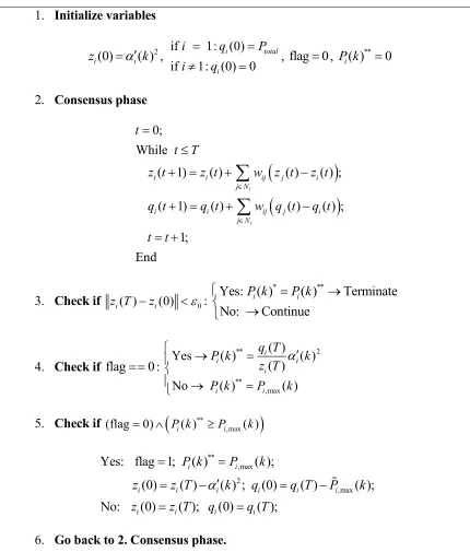
Table 2-1 shows the step-by-step algorithm for finding the optimal power allocation at the i -th node. The first step is initialization. For all i=1,..., N, the zi variable is initialized as ( ) and

qi is initialized as zero, except in one of the nodes where the q variable is initialized as Ptotal. Without loss of generality this node is indexed as 1.

The second step is the consensus phase. During this phase, each charging station updates its z

and q variables according to:





( 1) ( ) ( ) ( ) ,

i

i i ij j i

j N

z t z t w z t z t



  

_





( 1) ( ) ( ) ( ) ,

i

i i ij j i

j N

q t q t w q t q t



  

_

22

where Ni is the set of neighbors of node i, and wij=wji are connectivity strengths, which are chosen such that 0 ≤ < max

,.., | | . It can be shown that with this choice of

connectivity strengths, consensus values converge to the average of the initial values of all the nodes if the nodes form a connected group (i.e., if there is a path via neighbors between any two nodes) [16].

Equation (2-44) can also be represented in the matrix form as:

( 1) ( )

,

( 1) ( )

Z t Z t

W

Q t Q t

        _        (2-45) where,









( ) ( ) _N( ) T, ( ) ( ) _N( ) T

Z t  z t  z t Q t  q t  q t . (2-46)

and,

( , ) 1 , ( , )

i

ij ij

j N

W i i w W i j w



 

_

At steps 3, 4, and 5, each individual charging station uses the global information from the consensus phase along with its own local information to decide about its power allocation by calculating ( )∗∗ _as:

Equation (2-48) basically evaluates (2-21) by noting that consensus values have converged to the average of their initial values:

2 2 2 2 2 1 1 ( ) / ( ) ( ) ( ) . ( ) ( ) / ( )

i total i

i N i N total

i

j j

j j

q T P N k

k k P

z T

k N k

             





If ( )∗∗ _exceeds

, ( ), the charging station allocates , ( ) as the optimal allocation

of power and subtracts ( ) from its z variable and _, ( ) from its q variable to eliminate the information of charging station i in subsequent consensus phases. The charging stations

** ( ) 2

( ) ( ) . ( ) i i i i q T

P k k

z T 

23

Table 2-1: Cooperative Distributed PHEV/PEV Demand Management (CDPDM) Algorithm

1. Initialize variables

2

(0) ( )

i i

z k , if 1: (0) if 1: (0) 0

i total

i

i q P

i q

 

  , flag0,

**

( ) 0

i

P k 

2. Consensus phase









0; While

( 1) ( ) ( ) ( ) ;

( 1) ( ) ( ) ( ) ;

1; End

i

i

i i ij j i

j N

i i ij j i

j N t

t T

z t z t w z t z t

q t q t w q t q t

t t              





3. Check if z T_i( )z_i(0) ₀:

* **

Yes: ( ) ( ) Terminate

No: Continue

i i

P k P k

  



 

4. Check if flag 0:

** 2

**

,max

( )

Yes ( ) ( )

( )

No ( ) ( )

i

i i

i

i i

q T

P k k

z T

P k P k

        _{ } 

5. Check if





,max

(flag0) P ki( ) Pi ( )k

**

,max 2

,max

Yes: flag 1; ( ) ( );

(0) ( ) ( ) ; (0) ( ) ( );

No: (0) ( ); (0) ( );

i i

i i i i i i

i i i i

P k P k

z z T k q q T P k

z z T q q T

          

24

that have already reached their power limit ( _, ( )) will not change their power allocation in subsequent iterations of the algorithm. Step 6 of the algorithm closes the loop; the algorithm goes back to step 2 and another consensus phase starts. The distributed algorithm for each node will terminate if no change in the consensus values occurs after the consensus phase. Due to the cooperative distributed nature of this algorithm, we call it the Cooperative Distributed PHEV/PEV Demand Management (CDPDM) algorithm.

Remark 2-2:

One of the requirements for the proposed cooperative distributed algorithm is connectivity for the communications network. Considering that the power grid network and the power feeders form a physically connected system, the connectivity for the communications network can be realized by having a communications network similar to the physical power network.

2.5 Simulation Results and Analysis

This section presents the performance of the proposed distributed algorithm in section III under different case studies. In all the case studies, each charging station is running the cooperative distributed algorithm shown in Table II. The algorithm is initialized every Δt

25

determined by the charging level (e.g., 3.3kW for single-phase, level 2 charging) and battery constraints.

The first case study shows how the algorithm works during each optimization step, and the second case study considers the successive usage of the algorithm in the long run. The robustness of the algorithm to link/node failures is also tested. To make the demonstrations tractable, the number of charging stations in the first two case studies is kept at five. The communications topology between charging stations is chosen similar to the power network topology as shown in Figure 2-3 . If a single link/node fails in this topology, the rest of the graph will still remain connected and thus, the remaining nodes would be able to continue cooperation with others, via consensus.

The third experiment studies the scalability of the algorithm, and the fourth experiment studies the sub-optimality of the algorithm by benchmarking it against conventional centralized optimization methods. For these experiments, Monte Carlo simulations are used.

26

2.5.1 Case Study 1: Single–Step Optimization

A parking deck with five charging stations is considered. The objective is to optimally allocate the available power based on the priority of the vehicles. The priority for the i-th vehicle is set as:

1 ( )

( ) ( )

i

i i

w k

SoC k TtS k 





(2-50) where TtSi(k) is the amount of time, the i-th vehicle is going to stay at the charging station and

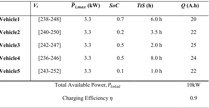
ε is a positive value introduced to avoid division by zero. Thus, the vehicles with lower SoC and sooner leaving time have higher priority for getting charged. At the kth time step, the information regarding the battery side of the vehicles is given in Table 2-2.

The maximum number of neighbors of each node is two, so according to the condition

0 ≤ < max

,.., | | , any connectivity strength between 0 and 0.5 can be chosen to

ensure stability. Using a small value for the connectivity strengths results in a slow convergence of the consensus algorithm. We set all the connectivity strengths equal to 0.4 which is in the feasible range for stability (0 < 0.4 < 0.5) and is not small. In general, the optimal selection of the connectivity strengths to achieve fast convergence, is itself an optimization problem that has been described in reference [38] and is outside the scope of this chapter. The sampling time for the consensus phase is 1msec and each consensus phase consists of 50 iterations.

27

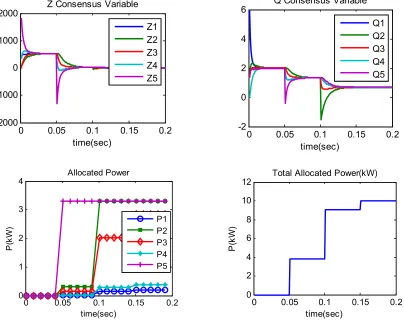
decrease. Consequently, the consensus variables converge to a new equilibrium point (their new average), which causes other charging stations to receive more power (because charging station 5 cannot consume any more power). Convergence to the new equilibrium is seen as big drops in the plots of the consensus variables. By the end of the second consensus phase (t = 0.1), charging station 2 reaches its maximum bound which allows other stations to receive more power. By the end of the third consensus phase (t = 0.15) all the available power is allocated and all the charging stations have received power in their feasible range. Therefore the consensus variables do not change any more and the algorithm settles down.

Now, we consider a link failure between node1 and node2 at time t = 0.01. Upon link failure, the two nodes can no longer exchange information with each other. When such a failure occurs, the connectivity strength between the two nodes becomes zero, namely = = 0.

Figure 2-5 shows the allocated power and the evolution of the consensus states. The charging Table 2-2: Information About the Vehicles in the 1st Case Study

Vt , (kW) SoC TtS (h) Q (A.h)

Vehicle1 [238-248] 3.3 0.7 6.0 h 20

Vehicle2 [240-250] 3.3 0.2 3.5 h 22

Vehicle3 [242-247] 3.3 0.5 2.0 h 25

Vehicle4 [236-246] 3.3 0.5 8.0 h 24

Vehicle5 [243-252] 3.3 0.1 1.0 h 22

Total Available Power, 10kW

28

stations can still converge to the same power allocation as shown in Figure 2-4 . As mentioned in Remark 2-2, the connectivity of the communications graph is the only requirement of the communications topology in order for the algorithm to work properly. This is the direct result of using consensus algorithms, which can work under switching topologies. After the link failure, the communications network remained connected, and the algorithm was able to failure, the communications network remained connected, and the algorithm was able to converge. However, due to the loss of a connection link, the convergence during the consensus phases had been slowed down, especially in the second and third consensus phases.

Figure 2-4: Allocation of power and evolution of consensus states for case study (1) with no link failure

0 0.05 0.1 0.15 0.2

-2000 -1000 0 1000 2000

Z Consensus Variable

time(sec)

Z1 Z2 Z3 Z4 Z5

0 0.05 0.1 0.15 0.2

-2 0 2 4

6 Q Consensus Variable

time(sec)

Q1 Q2 Q3 Q4 Q5

0 0.05 0.1 0.15 0.2 0

1 2 3 4

time(sec)

P

(k

W

)

Allocated Power

P1 P2 P3 P4 P5

0 0.05 0.1 0.15 0.2 0

2 4 6 8 10 12

Total Allocated Power(kW)

time(sec)

P

(k

W

29

2.5.2 Case Study2: Dynamic Optimization

In this part, we study the behavior of the algorithm in long run. The vehicles arrive and departure at different times. Moreover, for the vehicles inside the charging stations, parameters such as SoC and voltage change due to the charging process. So the optimization becomes dynamic and the single-step optimization problem to be solved (as in Case Study 1) keeps

Figure 2-5: Allocation of power and evolution of consensus states for case study (1) with single-link failure

0 0.05 0.1 0.15 0.2 -2000

-1000 0 1000 2000

Z Consensus Variable

time(sec)

Z1 Z2 Z3 Z4 Z5

0 0.05 0.1 0.15 0.2 -2

0 2 4

6 Q Consensus Variable

time(sec)

Q1 Q2 Q3 Q4 Q5

0 0.05 0.1 0.15 0.2

0 1 2 3 4

time(sec)

P

(k

W

)

Allocated Power

P1 P2 P3 P4 P5

0 0.05 0.1 0.15 0.2 0

2 4 6 8 10 12

Total Allocated Power(kW)

time(sec)

P

(k

W

30

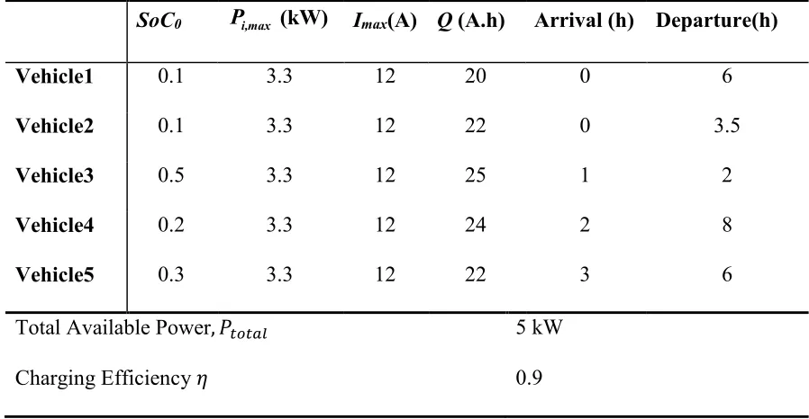
changing. Five vehicles with different initial SoCs and different arrival and departure times are considered as shown in Table 2-3 .

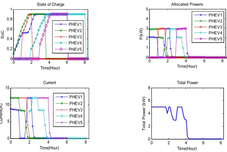
The desired SoC is 0.9 and the maximum power output of each station is 3.3kW. The priority weights are defined similar to case study1. We simulate the distributed charging control model for 8 hours. The charging stations change their power allocation every 10 minutes. Figure 2-6 shows the charging profiles of the vehicles over time. At time t = 0, two PHEVs are in the charging stations. PHEV2 has an earlier departure time and, therefore, gets higher charging rate. At time t=1h, PHEV3 arrives at the charging station. As PHEV3 needs to leave very soon, its priority for getting power is higher than those of PHEV1 and PHEV2. At this time PHEV1, which leaves later than the others, has the lowest priority. Therefore, its charging power drops to near zero, to allow PHEV3 to get more charging power. At time t=2h, PHEV3 leaves with

SoC=0.9. The allocation of power during the rest of the time can be explained similarly. We Table 2-3: Information About the Vehicles in the 2nd Case Study

SoC0 Pi,max (kW) Imax(A) Q (A.h) Arrival (h) Departure(h)

Vehicle1 0.1 3.3 12 20 0 6

Vehicle2 0.1 3.3 12 22 0 3.5

Vehicle3 0.5 3.3 12 25 1 2

Vehicle4 0.2 3.3 12 24 2 8

Vehicle5 0.3 3.3 12 22 3 6

Total Available Power, 5 kW

31

can see that at all times the total consumed power is below 5kW. The current profiles are drawn to show that the charging currents resulted from the optimization process are within the feasible boundaries (i.e., I ≤ Imax = 12A). This is done by translating the boundary on the charging current into a boundary on the charging power via multiplying it by the terminal voltage of the battery. This boundary then serves as a local constraint for the optimization problem.

Now, we consider the case where node2 fails to operate at t=0.5h and recovers at t=2h. Figure 2-7 shows the charging profiles under this scenario. Upon failure, node2 loses its connection with all its neighbors. However the rest of the nodes remain connected. When node2 fails, its charging rate drops down to zero and no change happens in the SoC of the vehicle. When node2 recovers at t=3h, PHEV2 starts to be charged again. . Similar to the case without node failure, all the local and global constraints are satisfied.

Figure 2-6: Charging profiles for case study (2) with no node failure

0 2 4 6 8

0 0.2 0.4 0.6 0.8 1

State of Charge

Time(Hour) S o C PHEV1 PHEV2 PHEV3 PHEV4 PHEV5

0 2 4 6 8

0 1 2 3 4 5 Time(Hour) P (k W ) Allocated Powers PHEV1 PHEV2 PHEV3 PHEV4 PHEV5

0 2 4 6 8

0 5 10 15 Current Time(Hour) C u rr e n t( A ) PHEV1 PHEV2 PHEV3 PHEV4 PHEV5

0 2 4 6 8

32 Remark 2-3:

To see why the algorithm is robust against single-link/node failures, we note that information exchange is happening through the consensus algorithm:





( 1) ( ) ( ) ( ) , 1...

i

i i ij j i

j N

z t z t w z t z t i N



  

_

The global information is the summation of local information:





1 1 1

( 1) ( ) ( ) ( )

i

N N N

i i ij j i

i i i j N

z t z t w z t z t

   

   





 

The second summation on the right hand side of the equation under balanced weights (i.e., , : _{ij ji}

i j w w

  ) always equals zero. Now if a link between two nodes i, j fails, the connectivity strength between those two nodes becomes zero (i.e., w_ij w_ji 0 ). Then still

Figure 2-7: Charging profiles for case study (2) with node failure

0 2 4 6 8

0 0.5 1

State of Charge

Time(Hour) S o C PHEV1 PHEV2 PHEV3 PHEV4 PHEV5

0 2 4 6 8

0 1 2 3 4 5 Time(Hour) P (k W ) Allocated Powers PHEV1 PHEV2 PHEV3 PHEV4 PHEV5

0 2 4 6 8

0 5 10 15 Current Time(Hour) C u rr en t( A ) PHEV1 PHEV2 PHEV3 PHEV4 PHEV5

0 2 4 6 8

33





1

( ) ( ) 0

i

N

ij j i

i j N

w z t z t

 

 

 

1 1

( 1) ( )

N N

i i

i i

z t z t

 

 





(summation of the local information) remains intact. Therefore, if the communications graph remains connected after the failure, the consensus values still converge to the true average (i.e., average of the global information). The proposed algorithm uses consensus networks to access the global information. Thus, it will be robust to any link failures that do not affect the connectivity of the communications networks. Also, when one node fails to communicate with its neighbors, then the rest of the group can continue their operations provided that their communications graph is connected.

2.5.3 Scalability Analysis

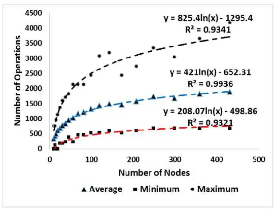
In this part of the article, we test the per-node computational scalability of the proposed distributed algorithm. To do so, we perform Monte Carlo simulations. Each node represents a charging station. The range for the number of nodes for the experiments is 10 to 450. For each value of the number of nodes, we ran 100 Monte Carlo simulations [39].

The parameters in each simulation are randomly sampled from their feasible ranges as shown in Table 2-4. A random network topology is chosen for each simulation. The number of operations each node needs to perform until reaching the optimal point, noperations, is calculated as follows:

,

operations out in

n n n k (2-53)

34

according to (2-44), each consensus operation involves k multiplications on average.

To count the number of outer loops, we count the number of times we have to repeatedly use (2-21) until all vehicles get a valid allocation of power. To count the number of inner loops, we look at the number of iterations the average consensus needs to reach within 2% of the final value. According to [38], this value can be calculated as:

ln(0.02) ln( ( ))

in n

W



 , (2-54)

where ρ(W) is the spectral radius of update matrix W in (2-45).

Figure 2-8 and Figure 2-9 show the minimum, maximum, and average number of the operations among 100 random simulations as a function of the number of nodes. The case studies are repeated for k  3 and k  20. Each dot in the figure corresponds to a set of 100 simulation data. A logarithmic trend line is fitted to the data points using a least squares error approach. The coefficient of determination (R2_{), with a maximum value of one, represents how} well the data is explained by the curve [40]. It can be seen that for both of the figures, the logarithmic trend explains the increase in the average computational complexity with R2=0.99.

Table 2-4: Monte Carlo Simulation Sampling Range

MinValue MaxValue

wi(k) 0 1

Qi 20A.h 30A.h

Vi(k) 210V 250V

SoC 0 1

35

In other words, by increasing the number of charging stations, the average computational complexity for the cooperative distributed algorithm grows almost logarithmically rather than exponentially. Therefore, the proposed distributed algorithm is scalable. By noting that each

Figure 2-8: Computational complexity of CDPDM algorithm as a function of number of nodes (average number of neighbors=3)

36

multiplication operation in the algorithm corresponds to a data-packet transfer between two nodes, the per-node communicational burden would exhibit exactly the same scalable behavior.

2.5.4 Sub-Optimality of the Algorithm due to Nonlinear Approximation: Benchmarking

against nonlinear optimization solvers

In this section, we study the sub-optimality of the solutions returned by the proposed algorithm due to the nonlinear approximation in section 2-3-2 by benchmarking it against two nonlinear optimization solvers: Sequential Quadratic Programming (SQP) and Interior Point methods. SQP methods are among the most successful nonlinear programming algorithms [41] and are used on nonlinear problems where the objective function and the constraints are both continuously differentiable. Interior Point methods are also conventional algorithms for solving constrained nonlinear optimization problems [42]. Both of these algorithms are provided by MATLAB through the fmincon optimization function.

37

alg i

%e_i J Ji 100,

J



  (2-55)

where Jalg is the objective function value returned using Algorithm 2-1, and Ji is the objective function value from the i-th algorithm (SQP or Interior Point).

The distributions of errors are shown in Figure 2-10 . We can see that the maximum deviation from optimality is around 2%.

2.6 Conclusion

In this chapter, we introduced a cooperative distributed energy management scheme for community charging of PHEV/PEVs. The main advantages of our approach are preventing the need for a central energy-management unit, being more robust against single-link/node failures, and being scalable in terms of single-node computations despite a small amount of sub-optimality (~2%). First, we formulated the charge allocation as a constrained nonlinear optimization problem and developed a procedure to solve the problem by checking KKT conditions. Then, we decomposed the charge information to local and global parts and

(a) (b)

Figure 2-10: Distribution of optimization error for CDPDM algorithm due to nonlinear approximation of the cost function with respect to a) the Interior Point method and b) SQP

-2 0 2

0 20 40

Percent Error(%)

F

re

q

u

e

n

c

y

-1 0 1 2

0 20 40 60

Percent Error(%)

Fr

e

q

u

e

n

c

38

proposed a distributed consensus-based algorithm to find the optimal charging policy in each charging time frame using peer-to-peer communications capabilities among charging stations. The performance, scalability, and robustness of the algorithm to single-link/node failures were case-studied.

To apply the proposed algorithm in the real world, practical issues such as EV and charging station communications features, voltage and frequency deviations at the terminals, losses in the power lines and feeders as well as more complicated battery models should be considered in the distributed optimization process. This will be the future work of the authors.

Acknowledgment: