Analysis of Projective-Iterative Methods for Solving Multidimensional Transport Problems

(1)

CONSTANTINESCU, ADRIAN C. Analysis of Projective-Iterative Methods for Solving

Multidimensional Transport Problems. (Under the direction of Dr. D.Y. Anistratov).

The particle transport equation has a wide range of applications: nuclear

engineer-ing, astrophysics, atmospheric science, medical physics, microelectronics manufacturengineer-ing, etc.

It is an integro-differential equation with seven independent variables: 3 spatial, 2 angular,

energy, and time, which cannot be solved analytically in most of the cases of interest. The

way to solve this equation is to discretize it in space, angle, energy, and time. In practical

cases, this leads to a huge sparse matrix. Iterative methods should be used even for solving

transport problems on the most powerful computers available nowadays. The need to

ana-lyze the behavior of these methods is obvious: knowledge about behavior of methods can

help us to improve them and avoid their use in cases in which they are not efficient. Also,

if we can predict what should happen in specific cases, we can verify and validate transport

codes. Analysis of iterative methods’ behavior in highly scattering and strong

heteroge-neous medium is very important from the point of view of solving various radiative and

particle transport problems. It became important for solving neutron transport equation

in full-core, due to current industry’s interest in obtaining very detailed transport solution

without homogenization. For these reasons, the main target of this thesis was to analyze

the convergence rate of four methods used to solve the steady state transport equation. We

were interested in studying behavior of these methods in case of one and two dimensional

strong heterogeneous and highly scattering medium with periodic structure, on rectangular

grids. In order to understand better these methods, we analyzed them as well in cases of

homogeneous and low scattering medium, uniform grids, etc. The main tool that we used

is Fourier analysis. Iteration matrix analysis was a secondary tool that we consider. It

proved to be restrictive in some cases but provided a good insight of the methods behavior.

In several difficult cases the Fourier analysis predicted degradation in efficiency or even

divergence for the methods that we’ve studied. In most of the cases, the numerical results

were consistent with the analytic predictions. In order to cover various areas where the

transport equation is used, we spanned wide ranges for parameters of transport equation.

Most of the cases in which the considered methods demonstrate slow convergence or even

(2)

by

Adrian C. Constantinescu

A thesis submitted to the Graduate Faculty of North Carolina State University

in partial fulfillment of the requirements for the Degree of

Master of Science

Nuclear Engineering

Raleigh

2006

Approved By:

Dr. D.Y. Anistratov Dr. Paul J. Turinsky

Chair of Advisory Committee

(3)

In memory of my father. . .

(4)

Biography

Adrian Constantinescu was born in 1976 in Bucharest, Romania. He graduated Nuclear

Power Engineering at Power Engineering Department, POLITEHNICA University of Bucharest

in 2000 and one year later he got his Master Degree in Modeling and Computer Based

Design in the same department. After a period of about 3 years, while he worked as

Teach-ing/Research Assistant at POLITEHNICA University, he decided to continue his education

in Nuclear Engineering at an American university. In August 2004 he started to work on

numerical methods for solving transport problems with Dr. Dmitriy Anistratov at NCSU.

(5)

Acknowledgements

The author would like to thank his adviser Dr. Dmitriy Anistratov for his valuable

advice and constant support. It was the first time and probably the last time he experienced

so long and fruitful discussions about numerical methods used to solve transport problems.

He also would like to thank his wife Cristina for all the patience and understanding

(6)

4.1 The Quasidiffusion Method for the 1D Transport Equation in Differential Form 61 4.2 The Quasidiffusion Method for the 1D Transport Equation in Discretized Form 62 4.2.1 Linearized Low-Order QD Equations in Discretized Form . . . 63 4.2.2 Fourier Analysis of QD Method in Infinite Heterogeneous Medium . 64 4.3 The Quasidiffusion Method for the Transport Equation in 2D Cartesian

Geometry . . . 68 4.4 The Quasidiffusion Method for the Discretized Transport Equation in 2D

Cartesian Geometry . . . 69 4.4.1 Linearized Low-Order QD Equations in Discretized Form . . . 71 4.4.2 Fourier Analysis of QD Method in Infinite Heterogeneous Medium . 73

5 Stability Analysis of First Moment Method 82

5.1 The First Moment Method for the 1D Transport Equation in Differential Form 82 5.2 The First Moment Method for the 1D Transport Equation in Discretized Form 83 5.2.1 Fourier Analysis of FM Method in Infinite Heterogeneous Medium . 83 5.3 The First Moment Method for the Transport Equation in 2D Cartesian

Geometry . . . 87 5.4 The First Moment Method for the Discretized Transport Equation in 2D

Cartesian Geometry . . . 87 5.4.1 Fourier Analysis of FM Method in Infinite Heterogeneous Medium . 88

6 Stability Analysis of Nonlinear Diffusion Acceleration Method 95

6.1 The Nonlinear Diffusion Acceleration Method for the 1D Transport Equation in Differential Form . . . 95 6.2 The Nonlinear Diffusion Acceleration Method for the 1D Transport Equation

in Discretized Form . . . 96 6.2.1 Numerically Estimated Spectral Radii for NDA in Infinite

Heteroge-neous Medium . . . 96 6.3 The Nonlinear Diffusion Acceleration Method for the Transport Equation in

(8)

6.4 The Nonlinear Diffusion Acceleration Method for the Discretized Transport Equation in 2D Cartesian Geometry . . . 99 6.4.1 Linearized Low-Order NDA Equations in Discretized Form . . . 100 6.4.2 Fourier Analysis of NDA Method in Infinite Heterogeneous Medium 101

7 Conclusion 104

(9)

List of Figures

2.1 PHI problem in 1D geometry . . . 15 2.2 Maximum eigenvalue vs. λfor SI with the DD transport discretization

pre-dicted by the Fourier analysis for PHI problem in 1D, ∆x1 = ∆x2 = 1,

Σt1 = Σt2 = 1,c1 = 1, andc2 = 0.1 . . . 19

2.3 Eigenvalues spectrum of SI with the short characteristics transport discretiza-tion for a 3_×3 homogeneous region with ideal and real BC, ∆x= ∆y = 1, and uniformc= 0.2 . . . 20 2.4 PHI problem in 2D geometry . . . 25 2.5 Maximum eigenvalue vs. λx and λy for SI with the short characteristics

transport discretization for PHI problem in 2D, Σt1 = 1 and Σt2 = 10−4 . . 27

3.1 Analytic spectral radii of SM with the DD transport discretization for PHI problem in 1D, ∆x= 1, c=0.9999 . . . 33 3.2 Analytic spectral radii of SM with the step method transport discretization

for PHI problem in 1D, ∆x= 1, c=0.9999 . . . 33 3.3 Analytic spectral radii of SM with the step characteristics transport

dis-cretization for PHI problem in 1D, ∆x= 1, c=0.9999 . . . 34 3.4 Numerically estimated spectral radii of SM with the DD transport

discretiza-tion for PHI problem in 1D, ∆x= 1, c=0.9999 . . . 35 3.5 Numerically estimated spectral radii of SM with the step method transport

discretization for PHI problem in 1D, ∆x= 1, c=0.9999 . . . 35 3.6 Numerically estimated spectral radii of SM with the step characteristics

transport discretization for PHI problem in 1D, ∆x= 1, c=0.9999 . . . 36 3.7 Eigenvalues spectrum of SM with the short characteristics transport

dis-cretization for a 3_×3 homogeneous region with ideal and real BC, ∆x = ∆y= 1, and uniform c= 0.9 . . . 39 3.8 Analytic spectral radii of SI and SM in 2D Cartesian geometry infinite

ho-mogeneous medium . . . 42 3.9 Analytic spectral radii of SM with the short characteristics transport

dis-cretization in infinite homogeneous medium . . . 47 3.10 Analytic spectral radii of SM with the DD transport discretization for PHI

(10)

3.11 Analytic spectral radii of SM with the step method transport discretization for PHI problem in 2D, ∆x= 1, ∆y= 1, c=0.9999 . . . 52 3.12 Analytic spectral radii of SM with the short characteristics transport

dis-cretization for PHI problem in 2D, ∆x= 1, ∆y= 1, c=0.9999 . . . 53 3.13 Numerically estimated spectral radii of SM with the DD transport

discretiza-tion for PHI problem in 2D, ∆x= 1, ∆y= 1, c=0.9999 . . . 53 3.14 Numerically estimated spectral radii of SM with the step method transport

discretization for PHI problem in 2D, ∆x= 1, ∆y= 1, c=0.9999 . . . 54 3.15 Numerically estimated spectral radii of SM with the short characteristics

transport discretization for PHI problem in 2D, ∆x= 1, ∆y= 1, c=0.9999 55 3.16 Maximum eigenvalue vs. λx and λy for SM with the short characteristics

transport discretization for PHI problem in 2D, Σt1 = 1 and Σt2 = 10−4 . . 55

3.17 Analytic spectral radii of SM with the short characteristics transport dis-cretization for PHI problem in 2D, ∆x= 1, ∆y1 = 0.1, ∆y2= 10, c=0.9999 56

3.18 Numerically estimated spectral radii of SM with the short characteristics transport discretization for PHI problem in 2D, ∆x = 1, ∆y1 = 0.1, ∆y2 =

10, c=0.9999 . . . 57 3.19 Structure of checker-board problem . . . 58 3.20 Numerically estimated spectral radii of SM with the short characteristics

transport discretization for checker-board problem in 2D, ∆x = 1, ∆y = 1, c=0.9999 . . . 58 3.21 Numerically estimated spectral radii of SM with the short characteristics

transport discretization for two regions problem in 2D, ∆x = 1, ∆y = 1, c=0.9999 . . . 60

4.1 Analytic spectral radii of QD with the step characteristics transport dis-cretization for PHI problem in 1D, ∆x= 1, c=0.9999 . . . 66 4.2 Numerically estimated spectral radii of QD with the step characteristics

transport discretization for PHI problem in 1D, ∆x= 1, c=0.9999 . . . 66 4.3 Analytic spectral radii of QD with the short characteristics transport

dis-cretization for PHI problem in 2D, ∆x= 1, ∆y= 1, c=0.9999 . . . 75 4.4 Numerically estimated spectral radii of QD with the short characteristics

transport discretization for PHI problem in 2D, ∆x= 1, ∆y= 1, c=0.9999 76 4.5 Analytic spectral radii of QD with the short characteristics transport

dis-cretization for PHI problem in 2D, ∆x= 1, ∆y1 = 0.1, ∆y2= 10, c=0.9999 78

4.6 Numerically estimated spectral radii of QD with the short characteristics transport discretization for PHI problem in 2D, ∆x = 1, ∆y1 = 0.1, ∆y2 =

10, c=0.9999 . . . 78 4.7 Numerically estimated spectral radii of QD with the short characteristics

transport discretization for PHI problem in 2D, ∆x = 1, ∆y1 = 0.1, ∆y2 =

10, c=0.9999, using cell average E’s . . . 79 4.8 Numerically estimated spectral radii of QD with the short characteristics

transport discretization for checker-board problem in 2D, ∆x= 1, ∆y1 = 1,

(11)

4.9 Numerically estimated spectral radii of QD with the short characteristics transport discretization for two regions problem in 2D, ∆x = 1, ∆y = 1, c=0.9999 . . . 81

5.1 Analytic spectral radii of FM with the step characteristics transport dis-cretization for PHI problem in 1D, ∆x= 1, c=0.9999 . . . 85 5.2 Numerically estimated spectral radii of FM with the step characteristics

transport discretization for PHI problem in 1D, ∆x= 1, c=0.9999 . . . 87 5.3 Analytic spectral radii of FM with the short characteristics transport

dis-cretization for PHI problem in 2D, ∆x= 1, ∆y= 1, c=0.9999 . . . 90 5.4 Numerically estimated spectral radii of FM with the short characteristics

transport discretization for PHI problem in 2D, ∆x= 1, ∆y= 1, c=0.9999 91 5.5 Analytic spectral radii of FM with the short characteristics transport

5.6 Numerically estimated spectral radii of FM with the short characteristics transport discretization for PHI problem in 2D, ∆x = 1, ∆y1 = 0.1, ∆y2 =

10, c=0.9999 . . . 92 5.7 Numerically estimated spectral radii of FM with the short characteristics

transport discretization for checker-board problem in 2D, ∆x = 1, ∆y = 1, c=0.9999, . . . 93 5.8 Numerically estimated spectral radii of FM with the short characteristics

6.1 Numerically estimated spectral radii of NDA with the step characteristics transport discretization for PHI problem in 1D, ∆x= 1, c=0.9999 . . . 97 6.2 Analytic spectral radii of NDA with the short characteristics transport

dis-cretization for PHI problem in 2D, ∆x= 1, ∆y= 1, c=0.9999 . . . 102 6.3 Analytic spectral radii of NDA with the short characteristics transport

(12)

List of Tables

2.1 Analytic and numerically spectral radii of SI for PHI problem in 1D, with Σt= 1,c1 = 1 and variablec2 . . . 17

2.2 Analytic spectral radii of SI with the DD transport discretization for PHI problem in 1D, with ∆x1 = ∆x2 = 1, Σt1 = Σt2= 1, c1= 1, and variable c2 19

3.1 Analytic spectral radii of SM with the DD transport discretization for PHI problem in 1D, ∆x= 1, c=0.9999 . . . 32 3.2 Analytic spectral radii of SM with the step method transport discretization

for PHI problem in 1D, ∆x= 1, c=0.9999 . . . 33 3.3 Analytic spectral radii of SM with the step characteristics transport

dis-cretization for PHI problem in 1D, ∆x= 1, c=0.9999 . . . 34 3.4 Numerically estimated spectral radii of SM with the DD transport

discretiza-tion for PHI problem in 1D, ∆x= 1, c=0.9999 . . . 34 3.5 Numerically estimated spectral radii of SM with the step method transport

discretization for PHI problem in 1D, ∆x= 1, c=0.9999 . . . 35 3.6 Numerically estimated spectral radii of SM with the step characteristics

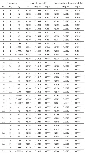
transport discretization for PHI problem in 1D, ∆x= 1, c=0.9999 . . . 36 3.7 Analytic and numerically estimated spectral radii of SM for PHI problem in

1D, with Σt= 1,c1 = 1 and variablec2 . . . 37

3.8 Analytic spectral radii of SM with the DD transport discretization for PHI problem in 1D, with Σt= 1,c1 = 1 and variablec2 . . . 39

3.9 Analytic spectral radii of SM with the short characteristics transport dis-cretization in infinite homogeneous medium . . . 46 3.10 Analytic spectral radii of SM with the DD transport discretization for PHI

problem in 2D, ∆x= 1, ∆y= 1, c=0.9999 . . . 51 3.11 Analytic spectral radii of SM with the step method transport discretization

for PHI problem in 2D, ∆x= 1, ∆y= 1, c=0.9999 . . . 52 3.12 Analytic spectral radii of SM with the short characteristics transport

dis-cretization for PHI problem in 2D, ∆x= 1, ∆y= 1, c=0.9999 . . . 52 3.13 Numerically estimated spectral radii of SM with the DD transport

(13)

3.14 Numerically estimated spectral radii of SM with the step method transport discretization for PHI problem in 2D, ∆x= 1, ∆y= 1, c=0.9999 . . . 54 3.15 Numerically estimated spectral radii of SM with the short characteristics

transport discretization for PHI problem in 2D, ∆x= 1, ∆y= 1, c=0.9999 54 3.16 Analytic spectral radii of SM with the short characteristics transport

3.17 Numerically estimated spectral radii of SM with the short characteristics transport discretization for PHI problem in 2D, ∆x = 1, ∆y1 = 0.1, ∆y2 =

10, c=0.9999 . . . 57 3.18 Numerically estimated spectral radii of SM with the short characteristics

c=0.9999 . . . 58 3.19 Numerically estimated spectral radii of SM with the short characteristics

4.1 Analytic spectral radii of QD with the step characteristics transport dis-cretization for PHI problem in 1D, ∆x= 1, c=0.9999 . . . 65 4.2 Numerically estimated spectral radii of QD with the step characteristics

transport discretization for PHI problem in 1D, ∆x= 1, c=0.9999 . . . 66 4.3 Analytic and numerically estimated spectral radii of QD for PHI problem in

1D, with Σt= 1,c1 = 1 and variablec2 . . . 67

4.4 Analytic spectral radii of QD with the short characteristics transport dis-cretization for PHI problem in 2D, ∆x= 1, ∆y= 1, c=0.9999 . . . 75 4.5 Numerically estimated spectral radii of QD with the short characteristics

transport discretization for PHI problem in 2D, ∆x= 1, ∆y= 1, c=0.9999 75 4.6 Analytic spectral radii of QD with the short characteristics transport

4.7 Numerically estimated spectral radii of QD with the short characteristics transport discretization for PHI problem in 2D, ∆x = 1, ∆y1 = 0.1, ∆y2 =

10, c=0.9999 . . . 78 4.8 Numerically estimated spectral radii of QD with the short characteristics

transport discretization for PHI problem in 2D, ∆x = 1, ∆y1 = 0.1, ∆y2 =

10, c=0.9999, using cell average E’s . . . 79 4.9 Numerically estimated spectral radii of QD with the short characteristics

c=0.9999 . . . 80 4.10 Numerically estimated spectral radii of QD with the short characteristics

5.1 Analytic spectral radii of FM with the step characteristics transport dis-cretization for PHI problem in 1D, ∆x= 1, c=0.9999 . . . 85 5.2 Numerically estimated spectral radii of FM with the step characteristics

(14)

5.3 Analytic and numerically estimated spectral radii of FM with the step charac-teristics transport discretization for PHI problem in 1D, with Σt= 1,c1 = 1

and variablec2 . . . 86

5.4 Analytic spectral radii of FM with the short characteristics transport dis-cretization for PHI problem in 2D, ∆x= 1, ∆y= 1, c=0.9999 . . . 90 5.5 Numerically estimated spectral radii of FM with the short characteristics

transport discretization for PHI problem in 2D, ∆x= 1, ∆y= 1, c=0.9999 91 5.6 Analytic spectral radii of FM with the short characteristics transport

5.7 Numerically estimated spectral radii of FM with the short characteristics transport discretization for PHI problem in 2D, ∆x = 1, ∆y1 = 0.1, ∆y2 =

10, c=0.9999 . . . 92 5.8 Numerically estimated spectral radii of FM with the short characteristics

transport discretization for checker-board problem in 2D, ∆x = 1, ∆y = 1, c=0.9999 . . . 93 5.9 Numerically estimated spectral radii of FM with the short characteristics

6.1 Numerically estimated spectral radii of NDA with the step characteristics transport discretization for PHI problem in 1D, ∆x= 1, c=0.9999 . . . 97 6.2 Numerically estimated spectral radii of NDA with the step characteristics

transport discretization for PHI problem in 1D, with Σt = 1, c1 = 1 and

variable c2 . . . 98

6.3 Analytic spectral radii of NDA with the short characteristics transport dis-cretization for PHI problem in 2D, ∆x= 1, ∆y= 1, c=0.9999 . . . 102 6.4 Analytic spectral radii of NDA with the short characteristics transport

(15)

List of Symbols and Abreviations

BC – Boundary Conditions

CG – Conjugate Gradient

DD – Diamond Differences

DSA – Diffusion Synthetic Acceleration

QD – Quasidiffusion

FM – First Moment

NDA – Nonlinear Diffusion Acceleration

PHI – Periodic Horizontal Interface

SI – Source Iteration

SM – Second Moment

TSA – Transport Synthetic Acceleration

(16)

Chapter 1

Introduction

1.1

Overview

Solving realistic transport problems has been, is, and will be a great challenge for

science & engineering community. The last decades were ones of important developments

in this area. However, no matter how much the tools for solving transport equation have

been improved, there will always be space for more, due to increasing needs in obtaining

more accurate solutions for more complicate problems as fast as possible.

The particle transport (linear Boltzmann) equation has a wide range of

applica-tions: nuclear engineering, astrophysics, atmospheric science, medical physics,

microelec-tronics manufacturing, etc. It is used to solve various problems: electron transport in

tomography, nuclear reactors assembly level calculations, full-core calculations, shielding,

radiative hydrodynamics with dynamic mesh, detection problems, photon transport in

at-mosphere, well-logging problems with unstructured mesh etc. Depending on the problem

that we solve, in addition to the transport equation we might need to solve some other

equa-tions related to the particular physics of the problem. Usually, this introduces nonlinear

terms, which complicate the problem even more. However, the structure of the transport

equation is the same no matter what problem we solve. For this reason we explored a wide

range for parameters of transport problems. Transport problem is not a new issue and

(17)

interested in this type of research. A good example is solving neutron transport problem

in full core. There is no method that can be used to solve efficiently this problem in 3D

(the number of coupled equations that have to be solved is O(1012_{)). There are methods}

that can solve this problem in 2D, by considering a small number of energy groups. One

of them is Nonlinear Diffusion Acceleration method, which is implemented in CASMO-4

code. However, this method loses effectiveness in case of optically thick cells. If we need

to consider a large number of energy groups, it is inevitable to have optically thick cells for

some energy groups.

The transport equation is an integro-differential equation with seven independent

variables: 3 spatial, 2 angular, energy, and time, which cannot be solved analytically in

most of the cases of interest. The way to solve this equation is to discretize it in space,

angle, energy, and time. In practical cases, this leads to a huge sparse matrix that cannot be

inverted directly in a reasonable amount of time, even if use the most powerful computers

available nowadays. The alternative is to use efficient iterative methods that takes advantage

of the structure of the transport equation. However, the standard method converges slow

in important cases.

The simplest method for solving iteratively the steady-state transport equation

is Source Iteration (SI) [16]. The method converges very slow if the medium is highly

scattering and optically thick (the particle suffers many scattering collisions before it is

absorbed). Fourier stability analysis in homogeneous medium has shown that the spectral

radius equals the scattering ratio c and the slowest convergent error mode of SI is the flat one, no matter what is the spatial dimensionality of the problem [2]. Consequently, people

have tried to develop methods that ”kill” this flat mode very quickly and accelerates the

other modes as well. Most of the methods have one common feature. Instead of calculating

the scalar flux directly as a weighted sum of the angular flux over all directions in the

SI fashion, they project the high-order problem (the transport equation) into a low-order

problem by applying 0th_{, 1}th_{, etc. moments to the transport equation, and define closure}

relationships. One complete iteration implies sweeping for the angular fluxes (high-order

solution) at intermediary step (s+ 1/2) and solving the low-order problem to get the scalar fluxes and currents at iteration (s+ 1). The low-order problem can be based on several steps, or can be formulated as one matrix equation. In the second case, the matrix of the

low-order problem is too large to be inverted directly. Thus, iterative methods are used,

(18)

definite matrices one can use Conjugate Gradient method). In some methods the low-order

problem is defined on a coarse mesh compared to the one used for the high-order problem.

After the low-order problem is solved the solution is reconstructed at fine mesh level.

As we’ve just mentioned, SI converges very slow in highly scattering medium,

which is common to many diffusive problems. In this case, the diffusion approximation

works and people tried to develop methods that make the angular flux error disappear

in one iteration if it is isotropic or linearly anisotropic. This can be done by introducing

special terms in the low-order problem, which are based on integrals over the angles that

are equal to zero (for linear terms) or to a constant (for nonlinear terms) in case of isotropic

or linearly anisotropic angular flux. In this regard, some methods use Legendre moments

of the angular flux. It was shown that the diffusion operator works well for this purpose.

As we see, there are ways to eliminate some particular error modes in exactly

one iteration and most of the methods use them. However, this is not enough to assure

fast convergence, or at least convergence. For instance, the Coarse-Mesh Rebalance method

proved to be divergent even in 1D geometry homogeneous medium [11] for optically thin and

thick cells. Also, First Moment method (FM) [22] with the diffusion coefficient proposed by

Lewis and Miller proved to be divergent in 1D geometry homogeneous medium for optically

thick cells.

1.2

Iterative Methods Used for Acceleration of the

Trans-port Equation

Regarding the low-order problem discretization we should say that any iterative

method can use a consistent discretization, which means the low-order equations are

de-rived from the discretized transport equation by applying directly the projection operator,

in discrete form to the discretized transport equation. In this case the method purely

ac-celerates the transport equation and the solution of the low-order problem is identical with

the solution of the discretized transport equation. If an independent discretization is used

the method produces high-order and low-order solutions that are different on finite grids.

If the width of the spatial cell tends to zero, then the two solutions tend to each other.

(19)

which is a disadvantage in multidimensional geometries because it is difficult to construct

fully consistent discretization of the low-order problem, and such discretizations sometime

lead to a system of equations that is very costly to solve.

Another important feature of these methods is linearity and nonlinearity. In case

of a linear method, the left hand side of the low-order equations contains the solution

at the current iteration, but the right hand side retains terms that are calculated based

on the solution from the transport sweep. In case of a nonlinear method the low-order

equations contain nonlinear terms, which in general are products of the solution at the

current iteration and some coefficients calculated based on the solution of the transport

sweep. If the grid is uniform a linear method will produce a symmetric positive definite

matrix that can be solved easily with Conjugate Gradient method. A nonlinear method will

generate an asymmetric positive definite matrix, which is harder to be solved. Sometimes

there are ways to mitigate this problem by symmetrization of the low-order equations in

differential form. Miften and Larsen [27] did that for Quasidiffusion method (QD). It is

possible to formulate a linear version of a nonlinear method for solving transport equation.

This results in a new method which behaves differently.

An important class of iterative methods is Synthetic Acceleration methods. These

methods can be formulated as preconditioners of the Richardson iteration. They are linear

and their low-order problem is formulated in terms of additive corrections. In order to

converge most of them require consistent discretization. One of the best known methods

from this class is Diffusion Synthetic Acceleration (DSA) [24]. In this case, the low-order

problem is basically a diffusion equation in terms of additive corrections for the transport

sweep solution. DSA converges only if the low-order problem is consistently discretized, or at

most a slightly inconsistent discretization is used. Probably the biggest disadvantage of DSA

is that it is hard to discretize consistently the low-order problem for multidimensional cases.

Larsen proposed a four-step algorithm for consistent discretization [23] that is supposed to

work for any discretization of the transport sweep.

Another method in this class is Transport Synthetic Acceleration (TSA) [28][29].

The low-order problem of TSA is a modified transport equation which contains a free

parameter β _∈ [0,1]. For β _∈ [0,1] TSA suppresses the flat error mode. The low-order problem is not solved directly. One may use SI method or an algebraic acceleration scheme.

A different class of methods is represented by Quasidiffusion and related

(20)

are formulated in terms of the solution. Also, they can be formulated in terms of

multi-plicative corrections. QD was proposed by Gol’din [18], and improved and analyzed later

[3][20][4][6][27]. For the particular case of incident flux boundary conditions (BC), Gol’din

and Chetverushkin introduced in [19] special BC for QD. Later, Miften and Larsen

pro-posed alternative BC [27] as well. QD is a nonlinear method that is based on the idea that

the Quasidiffuion (Eddington) factors, which close the low-order problem, are stable. In

case of isotropic and linearly anisotropic angular flux the Eddington factors are constant.

It was not proved that QD method is unconditionally convergent in homogeneous medium

for any type of independent discretization, but so far there have been no reports either

about slow convergence or divergence. QD proved to be fast convergent in 1D problems

and multidimensional problems as well, even in tough cases as up-scattering problems.

Second Moment (SM) method [22] can be considered as the linear version of QD

when the linearization is done around a flat solution [10]. The same as in case of DSA, the

diffusion equation is the basis for the low-order problem. SM has an important disadvantage

that makes it un-attractive: due to the spatial derivatives of second order Legendre moments

of the angular flux at iteration (s+ 1/2), it may give non-physical negative scalar fluxes. Lewis and Miller also proposed First Moment method (FM) [22]. FM can be formulated

for either additive corrections or multiplicative corrections. In the first case, if we use the

standard diffusion coefficient 1/3Σt and independent discretization, FM converges slow or

even diverges for 2D, infinite homogeneous medium. The reason is that it is equivalent

to DSA with independent discretization. A nonlinear version of FM is Nonlinear Diffusion

Acceleration (NDA) [31]. NDA method is implemented in CASMO-4 transport code [32][33].

It proved to be very efficient in full core calculations for optically thin cells.

Anistratov and Larsen [7] proposed a family of α-weighted iterative methods for slab geometry. They derived both nonlinear and linear versions of the methods. This

family of methods is a generalization of first flux [17] and second flux [21] methods. Fourier

stability analysis demonstrated that both linear and nonlinear methods are fast convergent

in 1D even if the low-order problem is independently discretized.

Another family of methods that don’t require consistent discretization is the one

proposed by Adams [1]. In his formulation, the transport sweep is accelerated by a system

of ”S2-like” equations, which are obtained by applying 0th angular moment to a differently

discretized high-order problem. Depending on the discretization of the S2-like equations,

(21)

found out that in 1D geometry it was fast convergent in all cases.

1.3

Stability Analysis. Tools

Stability analysis is an inherent part of any iterative method development. It is

performed to verify the behavior of iterative methods. Its results are also used to understand

how they works. This way the methods can be improved, or at least fixed for some particular

cases. Another application of stability analysis is verification and validation of the transport

codes. Using the analysis we can create sophisticated benchmark problems that can be used

to check whether a transport code, which uses that particular method, works properly or

not.

The main tool used in stability analysis is Fourier transformation. It can be used

for linear methods and for nonlinear methods that are linearized close to a solution. The

assumption that the error of the iterative solution can be expanded in Fourier series has to

be made. In homogeneous medium there is separation of variables (angular and spatial) and

the eigenfunction depends only on particle’s direction. Instead, in heterogeneous medium

there is no separation of variables, which means the eigenfunction depends on position as

well.

Zika and Larsen [38][39] have shown for 1D geometry what is the actual problem

that is analyzed in case of heterogeneous medium problem with periodic structure. Starting

from the transport equation and assuming the error modes can be written as product

of the eigenfunction and the complex exponential, they’ve derived a differential equation

with complex coefficients, whose solutions are the eigenfunctions. They considered periodic

eigenfunctions, but dxidn’t assume separation of variables. The resulting equations for

eigenfunctions were solved numerically.

An alternative to Fourier analysis in infinite medium is the iteration matrix

analy-sis for problems in finite domain. In this case, one formulates the iteration process in the

matrix form

x(s+1) =M x(s). (1.1)

(22)

yes how fast convergent it is. For linear methods constructing matrixM is straightforward. One can use this approach for nonlinear methods as well if the equations are linearized in

the vicinity of the solution. This method can be used to analyze the behavior of methods

in finite medium problems, but not in infinite medium problems. Note that in order to

evaluate the spectral radius ofM we need to invert the high-order and low-order operators. Hence, an important limitation is the size of the problem that we can consider due to limited

efficiency of the software we need for this analysis and hardware resources.

Sanchez [30] has shown that use of real periodic BC (BC for the transport equation

are solved using the outgoing angular flux from the previous iteration) increases the spectral

radius of the iteration matrixM, due to iteration on boundaries. When the optical thickness tends to 0, the spectral radius tends to 1. Sanchez also has shown that if we increase the

number of cells to_∞, the spectral radius ofM tends to the one given by Fourier analysis for infinite medium problem.

Regarding the analysis of nonlinear methods on heterogeneous problems, a

semi-analytic approach is possible. It was used by Yamamoto [37] for analysis of NDA in 1D

infinite heterogeneous medium. He linearized the method by frozen the nonlinear correction

factor and spanned the interval [₋1,1] for it. A more general approach is the following. We can linearize the nonlinear method around a non-flat solution and do the Fourier analysis

using the solution obtained with a transport code. In this case two questions arise. First,

how do we get the infinite medium solution? Second, can we get the solution of a problem for

which the method diverges? Regarding the first question, it is possible to use a combination

of reflective and periodic BC in order to obtain the solution of an infinite heterogeneous

medium with periodic structure. The answer of the second problem is affirmative too. For

small problems with reflective and/or periodic BC the method is likely to be convergent,

even if it is divergent for the infinite medium problem. The reason is that most of the error

modes are killed because it is a problem in finite domain with finite number of spatial cells

and specific BC. Even if the optical thickness of the region is small and the spectral radius

is very close to 1, there is no trouble. One can afford to do a large number of iterations in

order to get the infinite medium solution. Finally we should note that in infinite medium

problems the spectral radius of a nonlinear method depends on the solution, which means

it depends on the external source used for obtaining the solution. It is not the same for a

(23)

1.4

Homogeneous Medium Analysis

The behavior of each of the previously mentioned methods has been analyzed for

various scenarios. For DSA it was shown that, if a consistent discretization is used, it is

fast convergent in infinite homogeneous medium on rectangular grids in 1D [24] and 2D [2]

geometries as well. However, if an independent discretization is used we should expect slow

convergence or even divergence.

On the other hand, SM and QD methods can be used with an independent

dis-cretization [2]. It has not been proved that they converge fast in any scenario, but for

infinite homogeneous medium tests neither slow convergence nor divergence has been

re-ported so far. QD is a nonlinear method. One can analyze it by linearizing it close to the

solution. For homogeneous medium, the linearized equations are identical to SM written

for errors. Cefus and Larsen [10] have shown this identity for 1D and derived the

expres-sion of the spectral radius. As far as we know there are no published results regarding

Fourier analysis for SM method for 2D geometry in homogeneous medium. We derived the

expression of the spectral radius (see Chapter 3) in differential form and discretized form

using diamond differences (DD), step method and short characteristics discretizations of

the transport equation.

FM’s behavior has been analyzed by Lewis and Miller [22] for 1D geometry in

infinite homogeneous medium. They haven’t reported the spectral radii but only numbers of

iterations necessary for ONETRAN code to converge. On the other hand, Smith and Rhodes

[32] have reported a fast DSA-like convergence for NDA. Cho and Park [14] have analyzed

Coarse Mesh Finite Difference (CMFD) acceleration method in 1D geometry homogeneous

medium. For the case that the low-order problem is discretized on the same spatial mesh

as the transport equation, this method is equivalent to NDA. They’ve used an independent

discretization which lead to spectral radii grater than 1 in some cases. We’ve also tested an

independently discretized version of FM (using the standard diffusion coefficient) and we

found divergence for some 1D geometry homogeneous problems.

1.5

Heterogeneous Medium Analysis

DSA is one of the most analyzed methods for heterogeneous problems. The reason

(24)

multidimensional heterogeneous medium is Azmy’s proof [9] that there is no unconditionally

stable adjacent cell diffusive preconditioner weighted diamond differencing discretizations.

As example, he has shown that DSA loses effectiveness in Periodic Horizontal Interface

(PHI) problem (see [8]). Warsa, Wareing, and Morel [35] have shown that even a robust

version of DSA, which has been consistently discretized and found efficient in 3D geometry,

diffusive homogeneous medium, and unstructured grids [34], loses its efficiency in diffusive

and highly heterogeneous tests. They also have analyzed a slightly inconsistent version

of DSA (SQLA DSA), which proved to have a similar behavior. The conclusion of these

authors is that degradation in effectiveness is an inherent property of the analytical DSA

method. As a solution to fix this problem they proposed acceleration of SI using GMRES

method preconditioned by DSA [36].

TSA method has been analyzed in diffusive heterogeneous medium as well. Chang

and Adams [12][13] have observed not only degradation in TSA’s effectiveness but even

divergence. They’ve also found out that the spectral radii greater than 1 are given by real

negative eigenvalues. As a result, they proposed a modification of the method by embedding

TSA inside a Krylov solver as CG or GMRES.

NDA has been analyzed in 1D geometry heterogeneous medium by Yamamoto

[37]. Using the standard diffusion coefficient, he has found spectral radii greater than 1 for

many cases. The way Yamamoto has analyzed NDA was discussed in the previous section.

1.6

Thesis’ Objectives

The main objective of this research was to perform the stability analysis of two

nonlinear iterative methods used for solving the transport equation: QD and NDA, and their

linear versions: SM and FM. We’ve considered mono-energetic case, isotropic scattering,

1D and 2D Cartesian geometry, highly scattering and strong heterogeneous medium. To

discretize the transport equation we use DD, step method, and step characteristics schemes

in 1D geometry, and DD, step method, and short characteristics schemes in 2D geometry.

For the low-order problem we use a finite volume discretization. Mainly we are interested

in analysis of the methods that use step characteristics and short characteristics transport

discretizations. However, it is instructive to analyze the other two discretizations as well to

(25)

1.7

Main Results Presented for Defense

In this thesis we present the following results:

1. Fourier analysis of SM for 2D Cartesian geometry infinite homogeneous medium in both

differential and discretized form.

2. Iteration matrix analysis of SI (in 2D Cartesian geometry) and SM (in 1D and 2D

Cartesian geometries) in case of finite heterogeneous medium with periodic BC.

3. Fourier analysis of SI, SM, and FM for 1D geometry infinite heterogeneous medium.

4. Fourier analysis of SI, SM, and FM in case of 2D Cartesian geometry infinite

heteroge-neous medium with periodic structure.

5. Stability analysis of the nonlinear methods, namely QD and NDA in the vicinity of the

solution of infinite heterogeneous medium problem with periodic structure.

6. Numerically evaluation of SM, QD, and FM spectral radii in case of checker-board

problem and two regions problem for 2D Cartesian geometry.

1.8

Thesis’s Content

The remaining of this thesis is structured as follows. In Chapter 2 we analyze

the behavior of the SI method in 1D slab and 2D Cartesian geometries for heterogeneous

medium problems, using iteration matrix analysis and Fourier analysis. Chapter 3 presents

the analysis of SM and QD in 1D slab and 2D Cartesian geometries for heterogeneous

medium. In order to perform the Fourier analysis we linearize the low-order QD equations.

For SM we show the Fourier analysis in 2D geometry for infinite homogeneous medium in

both differential and discretized form. Chapter 4 presents the stability analysis of FM in

heterogeneous medium for 1D and 2D geometries. For NDA we derive the linearized

low-order equations around a non-flat solution in 2D geometry and perform Fourier analysis as

well. The thesis concludes with Chapter 5, where a final discussion regarding the results is

(26)

Chapter 2

Stability Analysis of Source

Iteration Method

In this chapter we present the iteration matrix analysis and Fourier analysis of the

SI method for heterogeneous medium in 1D slab and 2D Cartesian geometries. The results

of this analysis are used to compare SI and the other four iterative methods under

consid-eration. These comparisons are important in order to see whether the slowly convergent

error modes are dumped by the acceleration methods or not and whether other modes are

excited or not. We did iteration matrix analysis of SI in 1D and 2D. In this Chapter we

only show how we build the iteration matrix in 1D. The procedure for 2D is similar.

2.1

The Source Iteration Method for the 1D Transport

Equa-tion in Differential Form

The steady state transport equation for 1D geometry, mono-energetic case, isotropic

scattering and external source is:

µ∂ψ

∂x + Σt(x)ψ(x, µ) =

Σs(x)

2

1 Z

−1

ψ x, µ′

dµ′+Q(x)

(27)

wherex_∈[xL, xR],µ∈[−1,1] is the projection of particle’s direction vectorΩ on x-axis,~ ψ

is the angular flux, Σtis the total macroscopic cross section, Σsis the scattering macroscopic

cross section, andQis the external source. In order to solve this problem we need to specify BC. Vacuum BC in 1D are given by

  

ψ(xL, µ) = 0, µ >0,

ψ(xR, µ) = 0, µ <0.

(2.2)

Reflective BC in 1D have the form:

  

ψ(xL, µ) =ψ(xL,−µ), µ >0,

ψ(xR, µ) =ψ(xR,−µ), µ <0.

(2.3)

Periodic BC in 1D defined by:

ψ(xL, µ) =ψ(xR, µ), µ∈[−1,1]. (2.4)

SI for the transport equation in continuous form consists in a transport sweep that gives

one the angular flux at intermediary step (s+ 1/2):

µ∂ψ (s+1/2)

∂x + Σt(x)ψ

(s+1/2)₍_{x, µ}_{) =}Σs(x)φ(s)(x) +Q(x)

2 , (2.5)

and integration of the angular flux over all directions in order to get the scalar flux at the

next iteration (s+ 1):

φ(s+1)(x) =

1 Z

−1

ψ(s+1/2)(x, µ)dµ. (2.6)

Vacuum BC: _

 

ψ(xL, µ)(s+1/2) = 0, µ >0,

ψ(xR, µ)(s+1/2) = 0, µ <0.

(2.7)

Reflective BC: _

 

ψ(xL, µ)(s+1/2) =ψ(xL,−µ)(s+1/2), µ >0,

ψ(xR, µ)(s+1/2) =ψ(xR,−µ)(s+1/2), µ <0.

(2.8)

Periodic BC:

ψ(xL, µ)(s+1/2) =ψ(xR, µ)(s+1/2), µ∈[−1,1]. (2.9)

Thereafter, we refer to the above formulations of reflective and periodic BC as “ideal” BC. It

(28)

in one transport sweep. There is another version of these two types of BC, which are

actually used in the discretized versions of SI and most acceleration methods. Thereafter,

we refer to the above formulations of reflective and periodic BC as “real” BC. In this case

even for the given right hand side one needs to iterate in order to get the converged angular

flux, due to BC.

Real reflective BC:

  

ψ(xL, µ)(s+1/2) =ψ(xL,−µ)(s−1/2), µ >0,

ψ(xR, µ)(s+1/2) =ψ(xR,−µ)(s−1/2), µ <0.

(2.10)

Real periodic BC:

  

ψ(xL, µ)(s+1/2) =ψ(xR, µ)(s−1/2), µ >0,

ψ(xR, µ)(s+1/2) =ψ(xL, µ)(s−1/2), µ <0.

(2.11)

2.2

The Source Iteration Method for the 1D Transport

Equa-tion in Discretized Form

In order to discretize SI in 1D we need to define the spatial mesh _{xi−1/2, i =

1..N + 1, x1/2 =xL, xN+1/2 = xR} and the angular mesh µm, m= 1..Nm, whereN is the

number of the cells in the slab and Nm is the number of directions considered. Now we

can define the discretized solution: φi is the cell average scalar flux, ψm,i is the cell average

angular flux in ith _{cell for direction} _µ

m, and ψm,i±1/2 is the cell edge angular flux. In 1D

geometry discretized form of the SI method consists of a transport sweep (2.12), (2.13) and

evaluation of the average scalar flux at the next iteration (2.14)

µm

ψ_m,i(s+1₊₁/2)_/₂₋ψ_m,i(s+1₋/₁2)_/₂

∆xi

+ Σt,iψ(m,is+1/2) =

Σs,iφ(_is)+Qi

2 , (2.12)

ψ(_m,is+1/2) = 1 +αm,i

2 ψ

(s+1/2)

m,i+1/2+

1₋αm,i

2 ψ

(s+1/2)

m,i−1/2, (2.13)

φs_i+1=X

m

ψ_m,i(s+1/2)wm. (2.14)

Depending on the expression ofαmthe transport discretization corresponds to the following

methods:

1. The Diamond Differences

(29)

2. The step method

αm,i=µm/|µm|, (2.16)

3. The step characteristics

αm,i=

1 +e−

Σt,i∆_xi

µm

1₋e−

Σ_t,i∆_xi

µm

−_Σ2µm

t,i∆xi

. (2.17)

We can write the approximate solution at iteration s as the sum of the exact solution and the iterative error

ψ(_m,is+1/2) =ψm,i+δψ_m,i(s+1/2), (2.18)

ψ_m,i(s+1₊₁/2)_/₂ =ψm,i+1/2+δψ(_m,is+1₊₁/2)_/₂, (2.19)

φ(_is)=φi+δφ(_is). (2.20)

Hence, we can write SI method for the iterative error as

µm

δψ_m,i(s+1₊₁/2)_/₂₋δψ_m,i(s+1₋/₁2)_/₂

∆xi

+ Σt,iδψm,i(s+1/2) =

Σs,iδφ(_is)

2 , (2.21)

δψ(_m,is+1/2) = 1 +αm,i

2 δψ

(s+1/2)

m,i+1/2+

1₋αm,i

2 δψ

(s+1/2)

m,i−1/2, (2.22) δφs_i+1=X

m

δψ_m,i(s+1/2)wm, (2.23)

wherewm are the quadrature weights.

2.2.1 Fourier Analysis of SI Method in Infinite Heterogeneous Medium

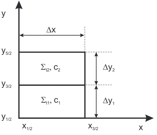
Let us consider a 1D version of the PHI problem [12]. This problem is defined by

two infinite layers of different materials repeated periodically. There is one spatial cell per

layer (see Fig. 2.1). We introduce the following ansatz:

δψ_m,i(s+1₊₂/2)_k = ωs˜am,ie−ˆiλxi+2k

δψ_m,i(s+1₊₁/2)_/₂₊₂_k = ωs˜_b_m,i_e−ˆiλxi+1/2+2k

δφ(_i₊₂s)_k = ωsAie−ˆiλxi+2k

(2.24)

(30)

needs to analyze only two neighborly cells to evaluate the eigenvalues ω. We consider only such discretizations for which αm,i is an odd function of µm. If we use the above ansatz

in Eqs. (2.21) and (2.22) written for two adjacent cells we find that ˜am,i has the following

form:

˜

am,i=A1

ae_m,i,₁+ ˆiao_m,i,₁+A2

ae_m,i,₂+ ˆiao_m,i,₂ (2.25) where superscriptsestands for even ando means odd, i.e.

µm=−µn⇒aem,i,j=aen,i,j,

µm =−µn⇒aom,i,j =−aon,i,j.

We don’t show here the expressions of a coefficients because of their complexity. Using (2.24) and (2.25) in Eq. (2.23) written for two adjacent cells we obtain a system of 2

equations for 2 unknowns: ω and A1/A2.      A1

A2ω =

P

m

A1

A2a

e

m,1,1+aem,1,2

wm

ω =P

m

A1

A2a

e

m,2,1+aem,2,2

wm

(2.26)

This system can be reduced to a second order equation inω that can be solved easily:

ω2

Ξ2,1 −

ωΞ2,2+ Ξ1,1

Ξ2,1

+Ξ2,2Ξ1,1 Ξ2,1 −

Ξ1,2 = 0, (2.27)

where Ξi,k=P m

ae_m,i,kwm. For every value ofλwe obtain two solutions forω. We evaluated

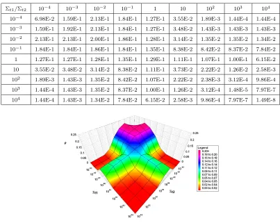
the spectral radii of the SM method in discretized form for PHI problem in 1D, non-uniform

scattering ratio c= Σs/Σt, but homogeneous Σt. The scattering ratio in the first cell was

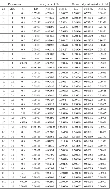
constant c1 = 1, but c2 varied. In Table 2.1 we show the analytic spectral radii of SM

obtained by means of Fourier analysis and the numerically estimated ones. We estimated

numerically the spectral radius inL2 norm ρ(s)= ||φ

(s)₋_φ(s−1)_|| 2 ||φ(s−₁₎

−φ(s−₂₎

||2

, (2.28)

x

1/2

x

3/2

x

S

t1

,

c

1

D

x

1

S

t2

,

c

2

X

5/2

D

x

2

(31)

using a 1000 cells slab, vacuum BC,Q= 1 for 250_≤x_≤750, Q= 0 in the rest of the slab,

ǫ= 10−₆

point-wise convergence criteria

max

i

1₋φ

(s+1)

i

φ(_is)

≤ǫ1₋ρ(s), (2.29)

We can see that SI is slowly convergent in most of the cases, especially when the scattering

ratio is high and the optical thickness of the cells (∆xΣt) is large.

2.2.2 Iteration Matrix Analysis of SI Method in Finite Heterogeneous Medium

In discretized form, ideal periodic BC for 1D geometry are defined as

ψ_m,(s+1₁_//₂2)=ψ_m,N(s+1₊₁/2)_/₂, m= 1..Nm. (2.30)

We can write (2.30) in terms of iterative errors as well

δψ(_m,s+1₁_//₂2)=δψ_m,N(s+1₊₁/2)_/₂. (2.31) In this case, Eqs. (2.21), (2.22), and (2.23) can be reduced to the following matrix form

A1δψ(s+1/2)=δφ(s), (2.32)

where δψ is the vector of all angular flux errors (both edge and average), and δφ is the vector of all average scalar flux errors. Eq. (2.23) written for all cells forms the following

system of equations

δφ(s+1) =A2δψ(s+1/2). (2.33)

This means the iteration matrix is

M =A2A

−1

1 . (2.34)

Periodic real BC for 1D geometry are given by:

  

ψ_m,(s+1₁_//₂2) =ψ_m,N(s−1₊₁/2)_/₂, µ >0,

ψ_m,N(s+1₊₁/2)_/₂ =ψ_m,(s−₁1_/₂/2), µ <0. (2.35)

We derive similar equations for the errors and form two matrix equations as above

(32)

Table 2.1: Analytic and numerically spectral radii of SI for PHI problem in 1D, with Σt= 1,

c1 = 1 and variablec2

Parameters Analyticρof SM Numerically estimatedρof SM ∆x1 ∆x2 c2 DD step m. step c. DD step m. step c.

(33)

δΦ(s+1)=A3δΦ (s+1/2)

, (2.37)

where δΦ is the vector of all angular flux errors (both edge and average), and all average scalar flux errors. Therefore, the iteration matrix is

M =A3A

−1

1 A2. (2.38)

We used the iteration matrix analysis to evaluate the spectral radii of SI for a 2

cells slab (see Fig. 2.1). We considered both ideal and real BC. The parameters of this

problem are the following: ∆x1 = ∆x2= 1, Σt1= Σt2 = 1, c1 = 1, c2 variable, and double

S4 GL quadrature. We built the iteration matrix in MATLAB 6.5, obtained the eigenvalues

ωi using function eig, and evaluated the spectral radius

ρ= max

i |ωi|. (2.39)

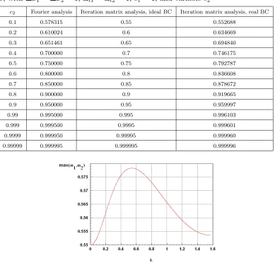
The analytic spectral radii are shown in Table 2.2. We included in the table the results of

Fourier analysis for infinite periodic medium problem with the same structure, to compare

the two types of analysis. In this particular case the iteration matrix has only 2

eigenfunc-tions and 2 eigenvalues. One of the eigenfunceigenfunc-tions is the spatially flat one, which means

that in some cases this type of analysis predicts exactly the spectral radius of SI for infinite

medium problems, if the ideal periodic BC are used. However, for c <0.7 we can see that iteration matrix analysis underestimates the spectral radius of the infinite periodic medium

problem. That can be explained by the fact that the slowest convergent error mode of the

infinite medium problem is not the flat one. In Fig. (2.2) we have the distribution of the

maximum eigenvalueω(for everyλwe get two solutionsω1andω2) with respect toλfor the

case c2= 0.1, which was obtained with the Fourier analysis. The spectral radius predicted

by the iteration matrix analysis with ideal BC is equal to ω(0), which corresponds to the flat error mode.

On the other hand, if SI with real periodic BC is considered then the iteration

matrix is not 2_×2 anymore because one needs to include in the vector of unknowns all

cell average scalar flux errors and all angular flux errors. We get extra error modes and

eigenvalues because the transport sweep has to iterate on BC. In case of optically thin

cells, this analysis will predict a spectral radius greater than the one of the infinite medium

problem. In our case, this happens for c2 >0.1. An interesting feature of real BC is the

(34)

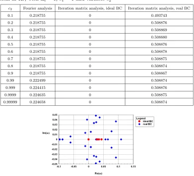
Table 2.2: Analytic spectral radii of SI with the DD transport discretization for PHI problem in 1D, with ∆x1 = ∆x2 = 1, Σt1 = Σt2= 1, c1 = 1, and variablec2

c2 Fourier analysis Iteration matrix analysis, ideal BC Iteration matrix analysis, real BC

0.1 0.578315 0.55 0.552688

0.2 0.610024 0.6 0.634669

0.3 0.651461 0.65 0.694840

0.4 0.700000 0.7 0.746175

0.5 0.750000 0.75 0.792787

0.6 0.800000 0.8 0.836608

0.7 0.850000 0.85 0.878672

0.8 0.900000 0.9 0.919665

0.9 0.950000 0.95 0.959997

0.99 0.995000 0.995 0.996103

0.999 0.999500 0.9995 0.999601

0.9999 0.999950 0.99995 0.999960

0.99999 0.999995 0.999995 0.999996

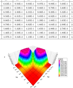
Figure 2.2: Maximum eigenvalue vs. λfor SI with the DD transport discretization predicted by the Fourier analysis for PHI problem in 1D, ∆x1= ∆x2= 1, Σt1= Σt2 = 1,c1 = 1, and c2 = 0.1

value of some complex eigenvalues had the same order of magnitude with the maximum

real eigenvalue. In Fig. 2.3 we show the spectrum of the eigenvalues in case of SI in

2D Cartesian geometry. We considered a homogeneous (Σt = 1) square region with 3×3

cells, uniform mesh ∆x= ∆y= 1, uniform scattering ratioc= 0.2, product quadratures set based on double S4 GL quadratures for azimuthal and polar angles, and short characteristics

discretization for the transport equation. We used both ideal and real periodic BC. As we

(35)

Figure 2.3: Eigenvalues spectrum of SI with the short characteristics transport discretization for a 3_×3 homogeneous region with ideal and real BC, ∆x= ∆y= 1, and uniform c= 0.2

eigenvalues. The conjugate of each complex eigenvalue is an eigenvalue also. Also, we note

that all complex eigenvalues have negative real part.

This type of analysis proved to be a very useful tool that can enable one to obtain

valuable information about the structure of the error modes and their eigenvalues in finite

problems. The Fourier analysis can be used to obtain upper bounds for the spectral radii in

finite medium problem. The practical problems are finite. That’s why it is very important

to know as much as possible about the structure of the iterative error modes in finite medium

problems.

2.3

The Source Iteration Method for the Transport Equation

in 2D Cartesian Geometry

The steady state transport equation for 2D Cartesian geometry, mono-energetic

case, isotropic scattering, and external source is

Ωx

∂ψ ∂x + Ωy

∂ψ

∂y + Σt(x, y)ψ

x, y, ~Ω= Σs(x, y) 4π

Z

4π

ψx, y, ~ΩdΩ + Q(x, y)

4π , (2.40)

wherex_∈[xL, xR],y ∈[yB, yT], Ωx is the x-component of particle’s direction vector ~Ω, Ωy

is the y-component of ~Ω, ψ is the angular flux, Σt is the total macroscopic cross section,

(36)

in 2D are defined as:             

ψ(xL, y, ~Ω) = 0 ,Ω~ ·~n(xL, y)<0,

ψ(xR, y, ~Ω) = 0 ,Ω~ ·~n(xR, y)<0,

ψ(x, yB, ~Ω) = 0 ,Ω~ ·~n(x, yB)<0,

ψ(x, yT, ~Ω) = 0 ,Ω~ ·~n(x, yT)<0,

(2.41)

where~n(x, y) is the outward normal vector and (x, y) is a point on the boundary. Reflective BC in 2D have the form:

            

ψ(xL, y, ~Ω) =ψ(xL, y, ~Ω∗) , Ω~ ·~n <0,

ψ(xR, y, ~Ω) =ψ(xR, y, ~Ω∗) , Ω~ ·~n < 0,

ψ(x, yB, ~Ω) =ψ(x, yB, ~Ω∗) , Ω~ ·~n <0,

ψ(x, yT, ~Ω) =ψ(x, yT, ~Ω∗) , Ω~ ·~n <0.

(2.42)

whereΩ~∗

is the exiting direction that reflects ontoΩ. Periodic BC in 2D are given by:~

  

ψ(xL, y, ~Ω) =ψ(xR, y, ~Ω) , ∀~Ω,

ψ(x, yB, ~Ω) =ψ(x, yT, ~Ω) ,∀~Ω.

(2.43)

SI consists in a transport sweep that gives us the angular flux at intermediate step

(s+ 1/2):

Ωx

∂ψ(s+1/2) ∂x + Ωy

∂ψ(s+1/2)

∂y + Σt(x, y)ψ

(s+1/2)_{x, y, ~}_Ω₌

Σs(x, y)φ(s)(x, y) +Q(x, y)

4π . (2.44)

The scalar flux is obtained by integrating the angular flux:

φ(s+1)(x, y) =

Z

4π

ψ(s+1/2)x, y, ~ΩdΩ. (2.45)

We also need BC.

Vacuum BC:             

ψ(s+1/2)(xL, y, ~Ω) = 0 , ~Ω·~n(xL, y)<0,

ψ(s+1/2)(xR, y, ~Ω) = 0 , ~Ω·~n(xR, y)<0,

ψ(s+1/2)₍_{x, y}

B, ~Ω) = 0 , ~Ω·~n(x, yB)<0,

ψ(s+1/2)(x, yT, ~Ω) = 0 , ~Ω·~n(x, yT)<0.

(37)

Reflective BC:             

ψ(s+1/2)(xL, y, ~Ω) =ψ(s+1/2)(xL, y, ~Ω∗) , ~Ω·~n <0,

ψ(s+1/2)(xR, y, ~Ω) =ψ(s+1/2)(xR, y, ~Ω∗) , ~Ω·~n <0,

ψ(s+1/2)(x, yB, ~Ω) =ψ(s+1/2)(x, yB, ~Ω∗) , ~Ω·~n <0,

ψ(s+1/2)(x, yT, ~Ω) =ψ(s+1/2)(x, yT, ~Ω∗) , ~Ω·~n <0.

(2.47)

Periodic BC: _

 

ψ(s+1/2)₍_x

L, y, ~Ω) =ψ(s+1/2)(xR, y, ~Ω) , ∀Ω~,

ψ(s+1/2)₍_{x, y}

B, ~Ω) =ψ(s+1/2)(x, yT, ~Ω) , ∀Ω~.

(2.48)

As in 1D, we define ”real” BC that are actually used to perform the transport sweep. Real

Reflective BC:             

ψ(s+1/2)(xL, y, ~Ω) =ψ(s−1/2)(xL, y, ~Ω∗) , Ω~ ·~n(xL, y)<0,

ψ(s+1/2)(xR, y, ~Ω) =ψ(s−1/2)(xR, y, ~Ω∗) , ~Ω·~n(xR, y)<0,

ψ(s+1/2)(x, yB, ~Ω) =ψ(s−1/2)(x, yB, ~Ω∗) ,Ω~ ·~n(x, yB)<0,

ψ(s+1/2)₍_{x, y}

T, ~Ω) =ψ(s−1/2)(x, yT, ~Ω∗) , Ω~ ·~n(x, yT)<0.

(2.49)

Real Periodic BC:

            

ψ(s+1/2)₍_x

L, y, ~Ω) =ψ(s−1/2)(xR, y, ~Ω) , ~Ω·~n(xL, y)<0,

ψ(s+1/2)(xR, y, ~Ω) =ψ(s−1/2)(xL, y, ~Ω) , ~Ω·~n(xR, y)<0,

ψ(s+1/2)(x, yB, ~Ω) =ψ(s−1/2)(x, yT, ~Ω) ,Ω~ ·~n(x, yB)<0,

ψ(s+1/2)(x, yT, ~Ω) =ψ(s−1/2)(x, yB, ~Ω) , ~Ω·~n(x, yT)<0,

(2.50)

2.4

The Source Iteration Method for the Discretized

Trans-port Equation in 2D Cartesian Geometry

To discretize SI in 2D we define the spatial mesh_{x_i₊₁_/₂, i= 1, Nx+ 1, yj−1/2, j=

1..Ny + 1}, and the angular meshµm, ηm, m= 1..Nm, where Nx is the cells number on

x-direction,Nyis the cells number on y-direction, andNmis the number of directions. Theµm

andηmare discrete directional cosines,φi,j is the cell average scalar flux,φi±1/2,jandφi,j±1/2

are the face average scalar fluxes,ψm,i,j is the cell average angular flux, andψm,i±1/2,j and

ψ_m,i,j±1/2 are the face average angular fluxes. SI method consists in a transport sweep and

evaluation of the average scalar flux at the next iteration:

φ(_i,js+1)=X

m

(38)

where wm are the quadrature weights. If we use WDD discretization the transport sweep

equations are:

µm

ψ_m,i(s+1₊₁/2)_/₂_,j₋ψ(_m,is+1₋/₁2)_/₂_,j

∆xi

+ηm

ψ_m,i,j(s+1/₊₁2)_/₂₋ψ_m,i,j(s+1/₋2)₁_/₂

∆yj

+Σt,i,jψ_m,i,j(s+1/2) =

Σs,i,jφ(i,js)+Qi,j

2 , (2.52)

ψ(_m,i,js+1/2)= 1 +α

x m,i,j

2 ψ

(s+1/2)

m,i+1/2,j+

1₋αx_m,i,j

2 ψ

(s+1/2)

m,i−1/2,j, (2.53)

ψ_m,i,j(s+1/2) = 1 +α

y m,i,j

2 ψ

(s+1/2)

m,i,j+1/2+

1₋αy_m,i,j

2 ψ

(s+1/2)

m,j,i−₁_/₂. (2.54)

For DD discretization αx_m,i,j =αy_m,i,j = 0 and for step method αx_m,i,j =µm/|µm|,αym,i,j =

ηm/|ηm|. Assuming as before that the approximate solution is the sum of the exact solution

and the iterative error, we can write all equations in terms of errors:

µm

δψ(_m,is+1₊₁/2)_/₂_,j₋δψ(_m,is+1₋/₁2)_/₂_,j

∆xi

+ηm

δψ(_m,i,js+1/₊₁2)_/₂₋δψ(_m,i,js+1/₋2)₁_/₂

∆yj

,

+Σt,i,jδψ(m,i,js+1/2)=

Σs,i,jδφ(i,js)

2 , (2.55)

δψ(_m,i,js+1/2) = 1 +α

x m,i,j

2 δψ

(s+1/2)

m,i+1/2,j+

1₋αx m,i,j

2 δψ

(s+1/2)

m,i−₁_/₂_,j, (2.56)

δψ_m,i,j(s+1/2) = 1 +α

y m,i,j

2 δψ

(s+1/2)

m,i,j+1/2+

1₋αy_m,i,j

2 δψ

(s+1/2)

m,j,i−1/2, (2.57)

δφ(_i,js+1) =X

m

δψ_m,i,j(s+1/2)wm. (2.58)

For short characteristics discretization we used linear interpolation of the incident

flux, between the angular fluxes in the two adjacent vertexes. The transport sweep equations

are

ξm,i,j=

µm∆yj

ηm∆xi

Quadrant I (µm >0,ηm >0)

τm,i,j= Σt,i,j

∆yj

ηm

,ψ∗ =ψ(_m,is+1₊₁/2)_/₂_,j₋₁_/₂(1₋ξm,i,j) +ψ_m,i(s+1−/12)/2,j−1/2ξm,i,j, for ξm,i,j ≤1,

τm,i,j= Σt,i,j

∆xi

µm

,ψ∗=ψ_m,i(s+1₋/₁2)_/₂_,j₊₁_/₂

1₋ 1

ξm,i,j

+ψ_m,i(s+1₋/₁2)_/₂_,j₋₁_/₂ 1 ξm,i,j

(39)

ψ(_m,is+1₊₁/2)_/₂_,j₊₁_/₂=ψ∗e−τm,i,j + 1₋e−τm,i,jΣs,i,jφ (s)

i,j +Qi,j

4Σt,i,j

. (2.59)

Quadrant II (µm>0, ηm<0)

τm,i,j = Σt,i,j

∆yj

−ηm

,ψ∗ =ψ_m,i(s+1₋/₁2)_/₂_,j₋₁_/₂(1₋ξm,i,j) +ψ(_m,is+1₊₁/2)_/₂_,j−1/2xim,i,j, forξm,i,j ≤1,

τm,i,j= Σt,i,j∆xi

µm

,ψ∗=ψ_m,i(s+1₊₁/2)_/₂_,j₊₁_/₂

1₋ 1

ξm,i,j

+ψ_m,i(s+1₊₁/2)_/₂_,j−₁_/₂

1

ξm,i,j

, forξm,i,j >1,

ψ(_m,is+1₋/₁2)_/₂_,j₊₁_/₂=ψ∗e−τm,i,j + 1₋e−τm,i,jΣs,i,jφ (s)

i,j +Qi,j

4Σt,i,j

. (2.60)

Quadrant III (µm<0,ηm<0)

τm,i,j = Σt,i,j

∆yj

−ηm

,ψ∗

=ψ(_m,is+1₋/₁2)_/₂_,j₊₁_/₂(1₋ξm,i,j) +ψ_m,i(s+1₊₁/2)_/₂_,j₊₁_/₂ξm,i,j, forξm,i,j ≤1,

τm,i,j = Σt,i,j

∆xi

−µm

,ψ∗ =ψ_m,i(s+1₊₁/2)_/₂_,j₋₁_/₂

1₋ 1

ξm,i,j

+ψ_m,i(s+1₊₁/2)_/₂_,j₊₁_/₂ 1 ξm,i,j

, forξm,i,j >1,

ψ(_m,is+1₋/₁2)_/₂_,j₋₁_/₂=ψ∗

e−τm,i,j _{+ 1}₋_e−τm,i,jΣs,i,jφ (s)

i,j +Qi,j

4Σt,i,j

. (2.61)

Quadrant IV (µm <0,ηm>0)

τm,i,j = Σt,i,j

∆yj

−ηm

,ψ∗ =ψ_m,i(s+1₊₁/2)_/₂_,j₊₁_/₂(1

Analysis of Projective-Iterative Methods for Solving Multidimensional Transport Problems

Contents

List of Figures

List of Tables

List of Symbols and Abreviations

Overview

Iterative Methods Used for Acceleration of the

Stability Analysis. Tools

Homogeneous Medium Analysis

Heterogeneous Medium Analysis

Thesis’ Objectives

Main Results Presented for Defense

Thesis’s Content

Chapter 2

The Source Iteration Method for the 1D Transport

The Source Iteration Method for the 1D Transport

The Source Iteration Method for the Transport Equation

The Source Iteration Method for the Discretized