Artificial Lumbered Flight for Autonomous Soaring.

POWERS, THOMAS CORNELIUS. Artificial Lumbered Flight for Autonomous Soaring. (Under the direction of Drs. Larry Silverberg and Ashok Gopalarathnam).

Soaring strategies are redefining the flight capabilities of small-class fixed-wing

UAVs. This dissertation presents an autonomous soaring strategy that exploits updraft energy

independent of the classification of an updraft. The strategy employs an artificial lumbered

flight algorithm (ALFA) that weighs near-field updraft velocity estimates and mission

priorities for navigation. This work raises the question of ALFA’s ability to handle classified updrafts. Indeed, ALFA does not explicitly consider the classification of the updraft. Instead,

ALFA measures updraft data along an aircraft’s flight path, estimates updraft data ahead of the

aircraft, generates candidate flightpaths ahead of the aircraft for evaluation, and then selects

the best candidate flightpath based on a reward function. This dissertation describes the

structure of ALFA and the tuning processes for the updraft estimator and the decision function.

Flight results demonstrate the ability of artificial lumbered flight to harness atmospheric energy

and complete its objectives. The flight results consider aircraft behavior in more detail,

examining ALFA’s effectiveness when flying among classified updrafts. They demonstrate the

ability of artificial lumbered flight to navigate unclassified updrafts and harvest energy from

thermal updrafts. Finally, this work highlights that autonomous flight design and control of

small-class aircraft is maturing into its own flight regime that lies between the flapping flight

© Copyright 2019 by Thomas Cornelius Powers

by

Thomas Cornelius Powers

A dissertation submitted to the Graduate Faculty of North Carolina State University

in partial fulfillment of the requirements for the degree of

Doctor of Philosophy

Aerospace Engineering

Raleigh, North Carolina

2019

APPROVED BY:

_______________________________ _______________________________ Dr. Larry Silverberg Dr. Ashok Gopalarathnam

Co-Chair of Advisory Committee Co-Chair of Advisory Committee

ii BIOGRAPHY

Thomas Cornelius Powers was born on September 5, 1988 in Woodland, California. After

spending 10 years of his childhood in the Netherlands, he attended Widefield High School in

Colorado Springs, and graduated in 2008. He attended Olivet Nazarene University in

Bourbonnais, Illinois, and graduated with a Bachelor of Science in Engineering in 2012. After

working for Case New Holland in the four-wheel drive tractor group for 14 months, he enrolled

in the direct-path PhD program at North Carolina State University in pursuit of Master and

Doctoral degrees in Aerospace Engineering. He earned his Master of Science in Aerospace

iii ACKNOWLEDGMENTS

First and foremost, I want to thank my wife Liz for supporting me throughout my studies and

for sacrificing to make this degree possible. We came to pursue a 2-year Master’s degree, and

5½ years later, I am finally getting ready to graduate. Thank you for all your help, support, and

encouragement throughout the time we have been here.

I also want to thank my co-advisors Dr. Silverberg and Dr. Gopalarathnam. Thank you

for all your guidance, support and insights as I lumbered through this degree, but also for the

career coaching and availability to talk about whatever I had going on. You have shared your

passions for research and flight, which I have come to share and will pursue for the rest of my

life. I also want to recognize my faculty committee, Dr. Ferguson and Dr. Lobaton. Thank you

for all your feedback and suggestions throughout this process.

I want to express my thanks to the members of the Flight Research Lab, who helped

me pick up the pieces after my many crashes and made sure my flight testing was a success.

Finally, a big thank you to my brother-in-law Cole Berkley for diving into flight control

iv TABLE OF CONTENTS

LIST OF TABLES ...v

LIST OF FIGURES ... vi

LIST OF SYMBOLS ... viii

Chapter 1: Introduction ...1

Chapter 2: Method ...6

2.1 The 3-DOF Model...6

2.2 The Reward Function ...9

2.3 Updraft Estimation ...11

2.4 Tuning the Reward Function ...13

2.5 Tuning the Updraft Estimation Method ...20

Chapter 3: Flight-testing Setup and Initial Results ...27

3.1 Flight Testing Setup ...27

3.2 Reducing the ALFA Flower...28

3.3 The Reward Pie ...30

3.4. Navigation Baseline ...31

3.5 Illustrative Flight ...32

Chapter 4: Detailed Flight Analysis ...37

4.1 Observed Behavior...39

4.2. Search and Return ...41

4.3 Circle Away ...43

4.4 Regional Loiter ...44

4.5 Sine Climb ...46

4.6 Loiter ...47

4.7 Thermal Loiter ...49

4.8 Angled Thermal ...51

4.9 Stationary Thermal...53

Chapter 5: Conclusions ...55

REFERENCES ...58

v LIST OF TABLES

Table 2.1 Aircraft Parameters: Phoenix 2000 Powered Glider ...13

Table 2.2 Performance Metrics for the Ridge Updraft Simulation ...16

Table 2.3 Performance Metrics for the Thermal Updraft Simulation ...18

Table 3.1 Sink Rates for Illustrative Flight Sections ...33

Table 4.1 Sink Rates for Detailed Flight Sections ...38

vi LIST OF FIGURES

Figure 2.1 The ALFA Flower...7

Figure 2.2 Free body diagram of the aircraft...8

Figure 2.3 The ALFA flight path matches the no-wind minimum glide slope ...14

Figure 2.4 Effect of navigation weight during a 30° approach to a ridge ...17

Figure 2.5 Effect of navigation weight when encountering a thermal ...19

Figure 2.6 Effect of updraft velocity on the transition wN...20

Figure 2.7 Test points for updraft estimation ...20

Figure 2.8 Updraft for testing and tuning the updraft estimation method ...22

Figure 2.9 Monte Carlo results for a single wind noise level with minimum MASE scores indicated ...23

Figure 2.10 The scaled error between estimated and measured updraft velocities along the flight path. ...24

Figure 2.11 Estimator performance at various locations about the aircraft ...25

Figure 2.12 Effect of sinusoidal flight path on updraft estimates ...26

Figure 3.1 Phoenix 2000 powered glider used for flight-testing ...27

Figure 3.2 The reward pie ...31

Figure 3.3 Altitude and flight path while prioritizing navigation ...32

Figure 3.4 Altitude flight profile ...33

Figure 3.5 Aircraft flight path over the test area ...34

Figure 3.6 Three-dimensional view of the illustrative flight...35

Figure 3.7 Detailed view on the 85-meter climb in section 1 ...36

Figure 4.1 The altitude profile of the flights ...38

Figure 4.2 Aircraft flight paths ...39

Figure 4.3 Eight common flight behaviors ...40

Figure 4.4 Left: Altitude profile for Search and Return. Right: Top view of flight path ...42

Figure 4.5 The flight path for Search and Return, with the reward pie at eight points along the path ...42

Figure 4.6 Left: Altitude profile for Circle Away. Right: Top view of flight path...43

Figure 4.7 The flight path for Circle Away, with the reward pie at eight points along the path ...44

Figure 4.8 Left: Altitude profile for Regional Loiter. Right: Top view of flight path ...45

Figure 4.9 The flight path for Regional Loiter, with the reward pie at eight points along the path ...45

Figure 4.10 Left: Altitude profile for Sine Climb. Right: Top view of flight path ...47

Figure 4.11 The flight path for Sine Climb, with the reward pie at seven points along the path ...47

Figure 4.12 Left: Altitude profile for Loiter. Right: Top view of flight path ...48

Figure 4.13 A 3D view of the Loiter flight path with the reward pie at six points along the path ...49

vii Figure 4.15 Left: Top view of the updraft measurement points and the contour of the

thermal. Right: A 3D view of the aircraft flight path ...51 Figure 4.16 Left: The altitude profile for Angled Thermal. Right: Top view of the flight path. 52 Figure 4.17 A 3D view of the Angled Thermal flight path with the reward pie at seven points

along the path. ... 52 Figure 4.18 Left: The altitude profile for Stationary Thermal. Right: Top view of the flight

path... 53 Figure 4.19 A 3D view of the Stationary Thermal flight path with the reward pie at seven

viii LIST OF SYMBOLS

, ,

x y z _{Aircraft position, m}

, ,

V   Velocity, m/s; Heading angle, rad; Velocity pitch angle, rad



m Aircraft mass, kg

g Gravitational acceleration, m/s2

Wx, Wy, U Wind velocity components, m/s T, L, D Thrust, N; Lift, N; Drag, N

t

 Iteration time, s

d Distance to waypoint, m

(

)

, , , P K U N

R R R R Potential, Kinetic, Updraft, and Navigation rewards, J , , ,

P K U N

w w w w Reward weighing coefficients

Sz Vertical component of GPS velocity, m/s

Fz Z component of fuselage elements of the direction cosine matrix 1, 2, 3, 4

a a a a Updraft estimation coefficients

e Updraft estimation error, m/s

C Updraft estimation robustness coefficient

n Moving window size

AR Aspect ratio

e Span efficiency factor

D

C Drag coefficient

K Number of data points used for MASE calculation

1

Chapter 1

Introduction

An entirely new approach to autonomous flight has emerged in recent years for aircraft in the

2-55 lb. class. This approach focuses on harvesting energy from the atmosphere to keep the

aircraft aloft instead of relying on onboard fuel sources as aircraft do today. The viability of

harvesting atmospheric energy autonomously is no longer in question [1-4] and will likely

drive aircraft design and control strategies for aircraft of this size in the future. Soaring flight

is generally characterized in two ways. Static soaring refers to the use of atmospheric updrafts,

which are typically classified as thermals produced by irregular ground heating and convection

currents, ridges caused by air moving up over large physical objects, and waves resulting from

passing over large physical features. Dynamic soaring uses wind speed gradients within the

boundary layer to help propel a bird or an unmanned aerial vehicle (UAV) and increase its

velocity.

While early research centered on the dynamic soaring flight of the albatross, recent

work has explored the benefits of static soaring. Toward this end, methods of estimating

vertical wind profiles and the development of wind exploitation strategies are being advanced.

Allen [1] presented an in-flight method of tracking a thermal’s center. When the thermal center

is known, he applies a circling strategy that harvests energy from the thermal while taking

measurements to keep track of where the thermal may be moving. Kahn [5] used an energy

variometer to get more detailed wind updraft measurements to aid in the locating and centering

around thermals. Langelaan et al. developed a few methods for estimating the wind field for

2 different methods of estimating the wind field such as using vehicle dynamics and kinematics,

computing wind from the vehicle response, and direct computation using GPS and airspeed

measurements. Other methods of estimating the wind field that have been used include using

an unscented Kalman filter, extended Kalman filter, Weibull probability density function and

a vision-based camera system [7-12]. Cheng and Langelaan [13] incorporated a guided

exploration component to actively search for favorable updrafts and map the wind field in

various regions with a flock of UAVs. Chakrabarty and Langelaan [14] explored orographic

or ridge lift with a heuristic search and created a regional energy map that the aircraft uses to

locate updrafts. Other studies focus on harnessing ridge lift to soar in urban environments, the

transition between multiple ridges, and using tree-based path planning approaches to navigate

the wind fields [15-19]. Langelaan and Bramesfeld [20] wrote a feedback controller that

enabled gust soaring, unlocking the potential of rapid wind changes to increase the energy of

an aircraft. All of these strategies focus on keeping the aircraft centered around the best area

of lift or developing methods for finding the next updraft quickly.

Path planning and exploration algorithms are used to incorporate wind and soaring

knowledge, thereby extending the lumbering flight capability of birds to UAVs. The A*

algorithm, which is used in path planning problems and aerial sense and avoid, is well suited

to a general auto-soaring approach, as suggested in a preliminary study by Chakrabarty and

Langelaan [14]. In that study, they used the A* algorithm to build an energy map of a region

which, in turn, they used to determine a path through a set of waypoints. Silverberg and Bieber

[21] imbedded the A* algorithm in a new central command architecture for large systems of

UAVs and recently flight-tested this with four aircraft. Other path planning algorithms used in

3 (RRT) and Look ahead Tree Search (LTS). Lawrance and Sukkarieh [22], Langelaan [23] and

Nguyen et al. [24] developed these methods and demonstrated good behavior in thermal and

ridge soaring applications in simulation. Gudmondsson et al. developed a lift seeking sink

avoidance algorithm based on a potential flow method and best path search method and

simulated flight through mountainous terrain [19]. Reinforcement learning strategies have also

been applied to enable a UAV to autonomously harvest energy from the atmosphere [25-27]

Since this area of work is relatively new, most of the literature simulates soaring

methods without flight-testing. However, there are several notable exceptions. Allen [1]

demonstrated his circling algorithm with successful flight tests, climbing an average of 172

meters in 23 thermal encounters. Edwards and Silverberg [2] entered an autonomously soaring

UAV in a soaring competition where it performed well against manually piloted gliders,

demonstrating the high potential of autonomously soaring UAV. Depenbusch et al. [3, 4]

showed the successful culmination of their research with autonomous soaring flights in their

two-part paper series, where they demonstrated successful wind estimation, classified updraft

identification, thermal mapping and exploration methods. Reddy et al. recently demonstrated

successful energy harvesting using their reinforcement learning approach [27].

While the term soaring encompasses the field of atmospheric energy harvesting, it

logically divides into a structured approach and a lumbered approach. The structured approach

is performed in three steps: exploration – identification – exploitation. The aircraft can use

knowledge of the wind field to guide exploration or can simply travel directly to its destination.

The aircraft identifies updrafts by comparing updraft velocity measurements with its database

of classified updrafts. Once the measurements match a classified updraft, the aircraft can

4 type of classified updraft based on knowledge of its structure. However, it relies on the

identification of a classified updraft and can only exploit updrafts that are contained in its

library.

The lumbered approach is a method of soaring that explores and exploits updrafts,

whether classified or not. Inspired by the lumbering flight of birds such as eagles and hawks,

which can only sense the nearby updrafts, this approach uses local, real-time decision-making

to navigate the wind field. The term lumbering refers to the lazy motion observed in the flight

of eagles and hawks when soaring through the air rather than when they flap their wings. This

approach eliminates the need for knowledge of updraft classifications and expands the scope

of energy harvesting to updrafts of all kinds, including unclassified updrafts. A drawback of

this method is that it does not tailor energy gain to specific updraft classifications.

Most of the literature studies autonomous soaring with the structured approach,

focusing on a single updraft classification. The lumbered approach has received little attention,

and its feasibility is still in question. It is uncertain how well this approach can use classified

updrafts such as thermals or ridges, and whether it is able to exploit unclassified updrafts at

all. For this reason, this work seeks to determine the ability of a real-time decision-making

process with limited wind field knowledge to gain energy from the atmosphere. The first goal

is to determine whether an aircraft can harness energy from the larger, classified updrafts

commonly exploited with structured autonomous soaring methods. The second goal is to see

if this method can harvest energy from the weaker, variable wind gusts, or unclassified updrafts

which are found in the space between large classified updrafts. This dissertation addresses

these questions using the Artificial Lumbered Flight Algorithm (ALFA). ALFA is a path

5 autonomous soaring. For this work, the ability to exploit energy from the atmosphere is

indicated by a decrease in aircraft sink rate from a straight gliding baseline. Thus, any reduction

in sink rate signifies successful updraft exploitation. This work describes ALFA’s development

and flight-testing and investigates the behavior and flight performance of ALFA as a test

aircraft navigates various wind fields. The focus of this dissertation is on the physical

implementation and flight testing of the algorithm as this allows the algorithm performance to

be assessed in a real, changing wind field. This is especially important when attempting to

harness the energy in unclassified updrafts. Finally, interesting flight patterns produced by the

6

Chapter 2

Method

ALFA employs a 3 degree-of-freedom (3-DOF) aircraft flight model that predicts a family of

candidate flight paths over an iteration in time. These predicted flight paths employ a real-time

estimate of the updraft velocity that is determined from updraft measurements over current and

previous iterations. A reward function weighs local (short-term) and global (long-term) goals

in the spirit of the A* path planning algorithms [28]. Based on this flight model, the algorithm

uses the reward function to select the best candidate flight path. This chapter first describes the

3-DOF model, the reward function, and the estimation of the updraft velocity. Then, it

describes the tuning of the reward function and of the updraft estimator.

2.1 The 3-DOF Model

Over each iteration, ALFA estimates a set of candidate flight paths using a 3-DOF model. This

family of candidate paths is referred to as the ALFA flower and a single flight path as the

flower’s petal (see Fig. 2.1). The 3-DOF model is governed by the 3-DOF equations of motion

for a fixed-wing airplane, shown in Eq. (1) [29]. The current work uses a 2-meter wingspan

powered glider as the test aircraft, which is described later in section 2.4, so the 3-DOF model

7 Figure 2.1: The ALFA Flower.

Each petal of the ALFA flower corresponds to the predicted flight path due to a set of

control inputs of pitch angle, bank angle and thrust level. The flower encompasses a range of

flight paths resulting from control inputs that span the flight capabilities of the aircraft. The

initial model has a set of pitch angles made up of four angles equally distributed between -15

to 15 degrees. The set of bank angles is composed of six angles spanning -60 to 60 degrees.

The thrust levels considered are the no thrust, half throttle, and full throttle levels. Using these

parameters, the equations of motion are numerically integrated using the second order

Runge-Kutta method over a relatively small iteration time step, i.e. 0.5 – 2.5 seconds. Simulating the

full ALFA flower over a 2 second iteration time step on a computer takes roughly 0.064

seconds. While simulating more candidate paths within the ranges of the parameters would

smooth the total combined flight path, it would be at the cost of greater simulation time. The

set of candidate paths shown here provide a good general starting point and is used in the

simulation of the algorithm. For flight testing, the candidate paths were simplified based on

8 Figure 2.2: Free body diagram of the aircraft

(1)





(

)

(

)

sin cos cos

x y

x V W

y V W

h V U

V T D mg

m

T L

mV

T L mg

mV                = + = + = + = − − = + = _ + − _

In Eq. (1), γ is the velocity pitch angle, the heading angle, φ, is the angle between the aircraft’s horizontal heading and North, and μ is the bank angle. The estimated wind velocity

components are Wx, Wy and U. Fig. 2.2 shows the free-body diagram of the aircraft. The estimated updraft profile and control inputs are assumed constant over the iteration time step

t, so the accuracy of the simulated flight path increases with a reduction in the size of the

iteration time step or by increasing the discretization of the input variables. In the simulations,

the iteration time step ranged from 0.5 – 2.5 seconds. During flight testing, a time step of 2

9 common for autonomous aircraft of the selected size. When the time step was shorter than 2

seconds, the aircraft exhibited abrupt and inefficient turns. When the time step was larger than

2 seconds, the control input did not update fast enough, resulting in large turns that lasted too

long and overshooting the desired turn. This turning behavior depends on the specific type of

aircraft selected, and other time step values may suit different aircraft.

2.2 The Reward Function

As mentioned earlier, the reward function considers both local and global goals. Locally, the

reward function considers the changes in the aircraft’s potential and kinetic energies and the

total “updraft kinetic energy” over the iteration time step. The updraft kinetic energy provides

a measure of the usable energy available in the surrounding wind field. Globally, the reward

function favors traveling toward the next waypoint. The global reward estimates the potential

energy reduction during a direct glide to the waypoint. The reward function is comprised of

four terms, each expressed in terms of energy.

(2)

R R

=

+

R

+

R

+

R

in which (3)

(

)

(

)

( )

(

)

(

)

2 1 Updraft 1

2

Global Navigation

P P i i

K K i i

U U i i

i i

N N

est

R w mg z z

R w m V V

R w U U

d d R w mg

L D + + + + +  = −    _{= −}    ₌   ₋  ₌  

10 priorities among the terms of the reward function, and ultimately govern the behavior of the

algorithm. Notice that these weights are not normalized. Also notice that the individual rewards are associated with the change in energy over an iteration time step; a large reward indicates a

correspondingly large improvement in the energy of the aircraft over the iteration time. The

exception is the updraft term, which just considers updraft velocity. Since the updraft term

reflects the kinetic energy contained in the atmosphere surrounding the aircraft, it must be

given a mass to bring the expression to energy units. However, it is unclear how mass of the

air should be represented in this situation. So, the mass is effectively absorbed into the updraft

coefficient wU. The tuning process sets the weights to produce the desired energy harvesting flight behavior, regardless of how the mass is included in the equations. If the mass were

calculated and included some other way, the value of the updraft coefficient that produces

desirable flight behavior would be different.

Lawrance and Sukkarieh [30] use a similar reward function in their paper to choose a

path from the set of candidate paths they produced using an expanding tree search. That reward

function uses the same potential, kinetic, and navigation terms as those shown in Eq. (3),

though they scale the terms with an exponential decay function rather than with coefficients as

shown here. Within the local considerations, they use an extra term which represents the

instantaneous power at the end of the flight segment,

K E



t

weight

K

instantaneous power term was replaced here with the updraft term to better represent and weigh

the impact of the vertical updraft velocity on the harvesting behavior. After choosing the path

11 the best petal repeats every iteration to produce a flight path that harvests energy from available

updrafts and can perform a desired mission.

2.3 Updraft Estimation

For successful lumbered flight, the reward function relies on an accurate estimate of updraft

wind velocity. Following the approaches discussed by Langelaan [6] and Premerlani [31], the

wind velocity components are estimated using the data from a typical IMU-GPS flight setup.

The updraft component U of the wind is

(4) , , 1

(

)

z i z i z i z i

S S V F F

U = + + − + +

where Sz is the vertical component of the GPS velocity, V is airspeed, and Fz is the z component of the fuselage elements of the direction cosine matrix. As indicated, they are evaluated at two

consecutive data points. Using estimated updraft velocity data at points along the flight path,

a fit of the wind is created from which the updraft velocity along the candidate paths is

extrapolated. Several assumptions serve to simplify this fit. Since the reward function primarily

differentiates between the candidate paths to the right and left of the aircraft, the updraft

estimator must be able to do the same. A first order fit meets this requirement. The fit also

assumes that the updraft velocity near the aircraft does not vary with altitude, which further

simplifies the fit. This assumption is reasonable because the updraft velocity varies little in the

direction of the flow, and the difference between the final altitudes of the candidate paths are

small compared to the forward distance travelled by the aircraft. Since both the velocity

changes and the distances between the path endpoints are small, any change in updraft velocity

due to altitude is negligible. While these assumptions are valid over a short distance ahead of

12 over time, the fit includes a time component to account for this movement. Thus, this

lower-order fit, which corresponds to a highly filtered fit, suits the ALFA application. More

specifically, the updraft velocity distribution is a function of x, y, and t and is represented as a moving plane that is tilted with respect to a horizontal plane. Its general form

(

)

(

)

1 2 x 3 y

U = +a a x v t− +a y−v t , is written as

(5)

U a

= +

a x a y a t

+

+

where

a

= −

a v

−

a v

The coefficients a1, a2, a3 and a4 are calculated at each iteration using a moving window. Employing Eq. (5), the measurement equations over the moving window are:

(6)

U

=

x a

+

e

(

i

=

1, 2,

, )

n









Equation (6) is n equations expressed in terms of four unknown coefficients at step j. In matrix form, the n equations at the jthstep and the augmented least square function are:

(7) U_j =X aT_{j j} +e_j T

(

) (

)

j j j j j j j

E =e e +C a −a − a −a −

in which =[ 1, 2, , ]

T

j n

U U U U and =[ 1, 2, ]

T T T T

j n

X x x x . Notice that the augmented least

square function has two parts – a least square error and a robustness term that penalizes changes

in the coefficients from the previous step. C is a weighing coefficient and aj-1 is the set of previously calculated coefficients. The minimization of Eq. (7) yields

(8)

(

) (

)

−

−

= + +

a X X X a

Notice that the weight C guarantees robustness since it guarantees that the matrix

(

)

has an inverse. The weight Calso eliminates large, rapid changes in the fit of the updraft wind

13 govern the behavior and success of ALFA. In preparation for flight-testing, these parameters

were tuned to produce desirable estimation and lumbered flight qualities, using the simulation

model as described in the next two sections.

2.4 Tuning the Reward Function

The aircraft used for simulations and flight-testing was the Phoenix 2000 powered glider. It is

a standard hobby-grade remote control glider with a built-in power system. Its interior space

housed the necessary equipment without being too large or having too much drag. Table 2.1

gives the aircraft’s physical parameters. The purpose of the simulations described below was

to tune the weights wP, wK, wUand wN of the reward function for this aircraft in the presence of a specified set of wind fields. The effect of the reward function weights and different wind

structures on the effectiveness of the flight paths was examined. The most suitable weights

from the simulation studies were then used in the flight-testing.

Table 2.1: Aircraft Parameters: Phoenix 2000 Powered Glider.

Weight (kg) 1.51

Average chord (m) 0.1715

Span (m) 2

Aspect ratio 11.62

0

D

C

The first step was to compare ALFA behavior with gliding-flight theory. For the

14 (9)

(

)

0

max

1

2 _D

ARe L D

C



=

For this simulation, ALFA was started for flight at an altitude of 500 m, heading east, and

flying horizontally at a speed of 9 m/s. This initial condition differs slightly from the inclined

speed for the best glide-slope. With these initial conditions, the reward function weights were

adjusted to achieve the result shown in Fig. 2.3. In the tuning process, the weights were found

to separate into a set that controls steady glide (wP and wK) and a set that enables energy harvesting (wUand wN). This separation of the reward weights simplified the tuning, allowing for greater focus on the ratio of the terms, rather than exact values each should have.

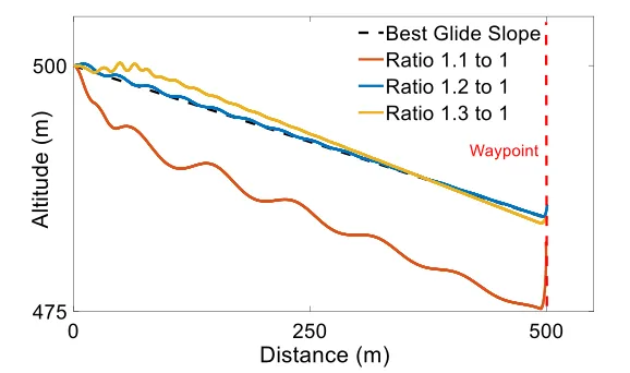
Throughout this tuning process, the potential and kinetic energy weights wPand wKwere found to have the greatest impact on the smoothness of the flight path. The ratio of wP to wK that produced the best glide flight path shown in Fig. 2.3 was 1.2 to 1.

Figure 2.3: The ALFA flight path matches the no-wind minimum glide slope.

As shown, the selected path with ratio 1.2 to 1 (shown in blue) oscillated slightly toward

15 the optimal glide slope. As shown, the oscillations settled down to the best glide slope,

represented by the dashed black line. The settling time of the oscillation can be decreased by

increasing the number of pitch angle values being considered in the AFLA flower, but at the

expense of computation time. When deviating from the 1.2 to 1 ratio, the flight path showed

increased oscillations and would not approach the best glide slope. When the ratio is less than

1.2 to 1, the kinetic energy of the aircraft generally dominates the path decision, causing the

aircraft to trade altitude for velocity, diving down sharply with long oscillations as seen in Fig.

2.3. When the ratio was greater than 1.2 to 1, the increased role of the potential term causes

the aircraft to climb while sacrificing velocity until the aircraft stalls and pitches down to regain

its velocity. The aircraft then settles to a more constant slope, but one less than the best glide

slope. Keeping the potential energy weight slightly higher than the kinetic energy weight

stabilized the flight path and prevented small wind disturbances from having such large

impacts.

After the ALFA flight paths matched optimal theory, simulated classified updrafts such

as ridges and thermals, were used to determine a set of updraft and navigation weights that

provide a balance between reaching the waypoint and harvesting energy. The emphasis of this

portion of the tuning process was finding values that allowed the aircraft to harvest energy and

gain altitude. The ratio of wUto wN was adjusted by changing the navigation term. In this study, ridge lift with a region of high updraft velocity of 5 m/s was simulated. The area of updraft is

modeled with a parabolic updraft velocity profile that runs the length of the ridge. This simple

model helps pinpoint the weight values at which the flight behavior transitions between either

harvesting energy or reaching the waypoint. It narrows down the weight values that produce a

16 cause the path to harvest energy and reach the destination is the starting point for further tuning

through flight testing. More elaborate ridge models have been developed for use with ridge

studies such as those discussed in [14-18], but the simple model suffices for this application.

As shown in Fig. 2.4, the ridge is oriented at a 30-degree angle to the line joining the

start point [at (0,0)] and navigation waypoint [at (300,0)]. When the navigation priority was

set too low as is the case with the harvesting path, the aircraft remains in the favorable updraft

along the ridge without proceeding to its waypoint. When the navigation priority was set too

high as shown with the navigation path, the flight path passed through the favorable updraft

while gaining minimal energy. The region of transition between the two behaviors is shown

when the navigation weight is 11 and the aircraft exploits significant energy from the ridge

before traveling the remaining distance to the waypoint. Finally, the baseline flight path

indicates the energy gained when gliding along a straight-line path to the waypoint. Table 2.2

provides a summary of the differences in flight paths using flight time, final energy, distance

traveled and reaching the waypoint as metrics for comparison. The flights were simulated for

a maximum flight time of 100 seconds.

Table 2.2: Performance Metrics for the Ridge Updraft Simulation.

Metric Baseline Harvesting σ Transition σ Navigation σ

WN ---- 3 11 18

Flight Time (s) 48 92.3 14.87 76.9 23.35 52.8 11.51

Energy (J) 1193.3 4347.8 1241.8 3130.5 1460.2 1609.1 738.3

Distance (m) 295.3 580.5 84.2 147.8 142.5 72.8 75.5

Reached

17 Figure 2.4: Effect of navigation weight during a 30° approach to a ridge.

ALFA’s ability to ride a ridge updraft successfully also depended on its approach angle to the

ridge. When the flight path approached the ridge at an angle greater than 70 degrees, the

algorithm did not differentiate between the right and left sides of the aircraft well enough to

turn and exploit the ridge updraft. ALFA demonstrated the ability to follow a ridge and circle

to harvest energy when the navigational priority was not set excessively high.

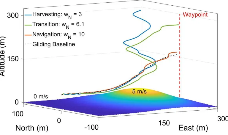
To study the effect of the navigation weights for a thermal updraft, a simulation was

conducted for a flight path that crosses a thermal (see Fig. 2.5). The set of weights that framed

the transition point between harvesting and reaching the waypoint for a classified ridge is

similar to the set of weights that frame the transition point for the classified thermal. This stems

from basing the algorithm on the measurement of updraft strength and decoupling it from the

identification of classified updrafts. For this simulation, the thermal was modeled as a vertical

column with a parabolic updraft profile. Like the ridge model, a simple model for a thermal

helps to narrow down the transition region between flight behaviors. More elaborate models

for thermals have been developed for in-depth simulations [1-3, 33-36]. When approaching a

18 was sufficiently low. As shown, the harvesting aircraft path circles the thermal, but does not

reach the destination. The navigation path travels directly to the destination without exploiting

much energy from the thermal. In the transition case, the aircraft exploits the thermal before

reaching the waypoint. The baseline flight path indicates the energy gained when gliding along

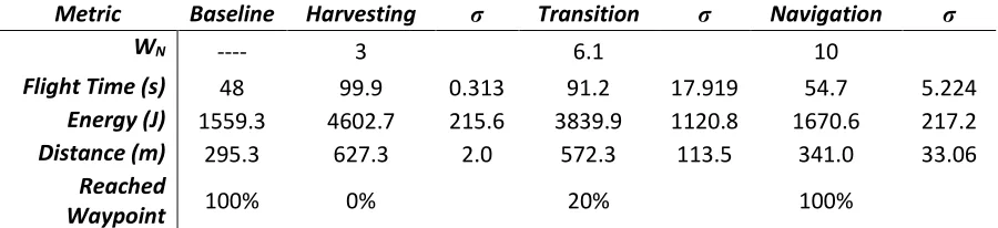
a straight line path to the waypoint. Table 2.3 provides a summary of the performance the

flights in Fig. 2.5. For these simulations, the maximum simulated flight time was 80 seconds.

In the rare situation when the aircraft approaches a thermal precisely toward its center, the

aircraft passes through it without engaging the thermal. Wind noise was added to this thermal

model as a random distribution with magnitude extremes of -0.1 to 0.1 m/s to evaluate the role

of wind noise on the flight behavior of the aircraft. Wind noise accounts for the changes in

updraft velocity that are rapid compared to changes in velocity due to the structure of a

classified updraft. In the first part of all three cases, the flight paths oscillated in response to

rapidly changing updraft velocity. As the updraft velocity from the thermal increases, it

overcomes the wind noise, allowing the updraft estimator to get better updraft measurements

and smoothing out the flight paths. These examples verified ALFA’s ability to achieve

desirable energy harvesting behavior without identifying classified updrafts. They also

provided a range of energy harvesting weights around the transition behavior of the flight paths

that serve as a starting point for further tuning the algorithm with flight testing.

Table 2.3: Performance Metrics for the Thermal Updraft Simulation.

Metric Baseline Harvesting σ Transition σ Navigation σ

WN _{---- 3 6.1 10}

Flight Time (s) 48 99.9 0.313 91.2 17.919 54.7 5.224

Energy (J) 1559.3 4602.7 215.6 3839.9 1120.8 1670.6 217.2

Distance (m) 295.3 627.3 2.0 572.3 113.5 341.0 33.06

Reached

19 Figure 2.5: Effect of navigation weight when encountering a thermal.

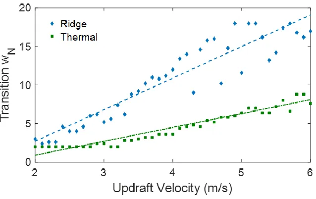
To understand the relationship between the maximum velocity of an updraft and tuning

parameters, Fig. 2.6 plots the last reward value at which the aircraft both harvests energy and

reaches its destination. This is indicative of the region in which transition takes place. In the

transition region, the reward function is balanced with the strength of the updraft. When this

happens, the stronger parts of the updraft cause the updraft term to dominate the reward value

of the candidate paths, making the aircraft stay in the high lift area. For any given updraft

velocity, the aircraft will stay in the region of updraft for wN values below the transition value, and the aircraft will reach the waypoint for wN values above the transition value. For both ridges and thermals, as the maximum updraft velocity increases, the aircraft needs a stronger

navigation weight to pull the aircraft out of the updraft. When navigating real updrafts, which

tend to get weaker with increasing altitude or time, the aircraft will break out of the updraft

when the updraft velocity sinks below the velocity corresponding to the selected transition

20 Figure 2.6: Effect of updraft velocity on the transition wN.

2.5 Tuning the Updraft Estimation Method

To ensure that the method of fit used to estimate the updraft velocity ahead of the aircraft is

accurate, the estimation of updraft velocities was simulated at five points around the front of

the aircraft (see Fig. 2.7). As shown, the points formed a semi-circle of radius r around the aircraft.

Figure 2.7: Test points for updraft estimation.

21 aircraft can update updraft measurements at 3 Hz, and the nominal gliding speed for the aircraft

is just over 9 m/s, r was set to 3 meters to simulate the distance traveled between measurements. The window size n and the weight C were tuned based on this setup.

When performing the tuning, the first simulation started with a constant updraft

velocity that stepped up to a higher velocity halfway along the flight path to see the updraft

estimation’s peak-overshoot and settling time characteristics. This addressed the estimation

problem along a straight-line flight path. Next, the estimation problem was extended to

two-dimensional space. Here, the problem considered a thermal updraft with a maximum strength

of 8 m/s, as shown in Fig. 2.8. Noise in the wind velocity was added to the model by adding a

sinusoidal noise function to the updraft distribution. This sinusoidal noise function was given

an amplitude that ranged from 0 – 0.5 m/s, and period that ranged from 0.1 meters to 2 meters.

The noise is always modeled as noise in the vertical direction. The amplitude and period of the

noise function were adjusted throughout the testing to simulate various noise conditions. The

sampling rate along the flight path coupled with the period of the noise function produced a

noise profile that appeared random. Two flight paths were simulated through the thermal, one

straight, and one sinusoidal, to compare the performance of the updraft fit in the regions to the

left and right of the aircraft. The sinusoidal path had an amplitude of 10 meters and a period of

40 meters. The updraft estimates along the straight flight path were compared with the updraft

estimates along the sinusoidal flight path to help determine the importance of data points

22 Figure 2.8: Updraft for testing and tuning the updraft estimation method (Umax = 8 m/s).

The tuning process considered the updraft estimator performance at each of the six

locations around the aircraft. The effect of changing the parameters n and C was studied. Increasing n and C were both found to increase lag (settling time), but there was a tradeoff between the lag and filtering the wind noise out of the signals. The primary effect of the

weighing coefficient C was in preventing large overshoot errors. The primary effect of the size of the moving window n was to filter out wind noise. With the effect of the parameters identified, Monte Carlo simulations were run to choose the parameters.

Since the parameters must be suited to many flight conditions, a metric was needed to

compare the estimation error during various situations. These situations considered various

levels of wind noise and considered the error at the six estimation locations discussed above.

Since the updraft error is dependent on the magnitude of the updraft velocity, the metric had

to be normalized to eliminate that factor. The Mean Absolute Scaled Error (MASE), which

normalizes the average error with the magnitude of the updraft velocity in order to weigh the

23 (10) 1

1 2 1 K k k K k k k e MASE K U U K = − = = − −





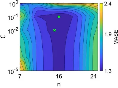
In Eq. (10), K is the number of total data points, ek is the error between the estimated and measured updraft velocities, and Uk is the updraft velocity at a given point. The results show the MASE values for a range of n and C for the simulated sinusoidal flight path for all of the six locations at one level of wind noise (see Fig. 2.9). The minimum MASE score for

this case is indicated by the green dot. The other simulations, which considered multiple

strengths and types of noise and varying levels of sinusoidal flight, were run and the combined

minimum MASE value is indicated by the green x. This combined minimum MASE value

indicates the chosen parameters of n = 15, and C = 0.01.

24 Using these parameters, Fig. 2.10 shows the error between the estimated and actual

updraft that has been scaled by the magnitude of the updraft velocity along the flight path.

When measuring at the aircraft, the error is below 2% for 93% of this flight path. The calculated

R2 value for the flight path is 0.991. This indicates that the updraft estimator should be sufficient for extrapolating the updraft values.

Figure 2.10: The scaled error between estimated and measured updraft velocities along the flight path.

To help visualize the effect and performance of the selected parameters, Fig. 2.11

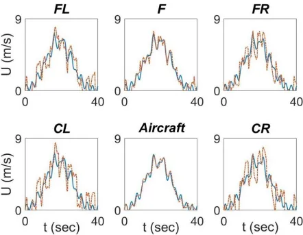
shows the measured updraft velocities (solid blue line) and estimated updraft velocities (dashed

orange line) along the simulated sinusoidal flight path for each of the six locations. The updraft

distribution includes wind noise with a strength up to 0.5 m/s. As shown, the estimate at the

aircraft, where the sensor is located, is better than at the other 5 points. Also shown, the

estimate at F is better than along the left and right sides of the aircraft. The updraft estimates at points FL, FR, CL, and CR were the least accurate. This indicates that the data is not “rich”. The “richness” of the data describes whether the data has enough points orthogonal to the flight

path to generate a realistic 2-dimensional updraft model. A model that produces small errors

25 later, a sinusoidal flight path improves the richness of the data, but even so, the aircraft’s

inability to measure data outside the flight path of the aircraft produces richness concerns.

However, the data did show that there is a distinction between the left and right sides of the

aircraft, which is necessary for successful energy harvesting.

Figure 2.11: Estimator performance at various locations about the aircraft.

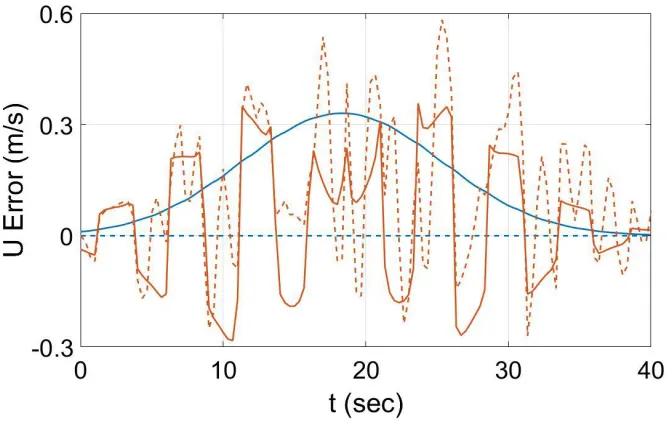
Now that the updraft estimation parameters are set, the differentiation between left and

right sides of the aircraft were analyzed to ensure the reward function could differentiate

26 color) and its improvements over the simulated straight flight path (blue color). The solid lines

indicate measured difference in updraft velocity between the two locations, and the dashed

lines show the estimated differences. While the measured velocities of the straight path

differentiated between the right and left sides, its estimated velocities did not register a

difference at all. When the aircraft followed a sinusoidal path, however, the estimated

velocities matched the measured velocities much better. This indicates that data richness

affects the success of the estimator and, if needed, prescribing a sinusoidal flight path can

produce better results. The estimates still overshoot changes in updraft velocity, but this

behavior is expected. Since the algorithm only needs to differentiate between the two sides of

the aircraft, the presence of exaggerated values can be beneficial.

27

Chapter 3

Flight-testing Setup and Initial Results

3.1 Flight Testing Setup

The test platform for ALFA was the Phoenix 2000 EPO Composite R/C Glider (see Fig. 3.1).

It has a two-meter wingspan foam wing, with the option of landing flaps, a 1.16-meter-long

blow-molded fuselage and is powered by a 1050KV brushless motor and folding propeller. A

powered glider was selected for ease of launch and recovery. Its loaded flight weight was 1.51

kg.

Figure 3.1: Phoenix 2000 powered glider used for flight-testing.

A flight controller (Pixhawk Mini) was used in conjunction with an open-source ground

control software (Mission Planner) to control the aircraft, and communication between the

aircraft and the ground control station (GCS) was accomplished with RFD-900 telemetry units.

28 to the aircraft. The flight data presented in this dissertation was collected in September 2018

at the North Carolina State University Lake Wheeler Road Field Laboratory. The flight area

consisted primarily of cornfields, with some trees around the border and a couple of buildings

and trees in the center. The rolling fields allowed for good thermal activity in the mornings and

afternoons. Throughout flight-testing, the reward function weights were adjusted to produce

desirable flight behaviors depending on the wind conditions. Several flights were conducted

with a set of weight values, and based on the behavior of the aircraft, the ratio was adjusted to

find the set of values that produced energy harvesting behavior. This process was repeated

every flight day as the wind conditions were a large factor in which sets of weights would

produce energy harvesting behavior. Over time, the parameter values were slightly adjusted

until the desired energy harvesting behavior was observed. This resulted in a wU to wN ratio of 5 to 1. Adjusting the iteration time step to a length of 2 seconds also helped produce smooth

energy harvesting flight behaviors.

3.2 Reducing the ALFA Flower

Before conducting flight tests, there are several considerations which allow the ALFA flower

to be reduced to fewer candidate paths, which in turn will improve the simulation time. Recall

that the reward function consists of four terms: potential, kinetic, updraft, and navigation. The

potential and kinetic energy terms primarily address the aircraft’s ability to maintain a steady

glide, as discussed previously. During flight-testing, the purpose of the flight controller is to

maintain steady glide and govern the flying characteristics of the aircraft, effectively handling

the potential and kinetic terms. This leaves the updraft and navigation terms for the ALFA

algorithm to control. Letting the flight controller manage the steady glide components of the

29 function, as they govern the steady glide of the aircraft in simulations. If ALFA was fully

implemented on the flight controller, all four terms would be governed by the reward function

as well. However, since the algorithm is run on the ground station, it is logical to let the flight

controller handle the terms it already governs. This consideration in addition to the

assumptions made in the updraft estimation process, namely that updraft velocity is

independent of altitude, allows the ALFA flower to be reduced to one pitch value producing

nearly planar flight. The second reduction is the removal of thrust levels from the candidate

paths. Since the focus of this dissertation is to investigate the energy harvesting capabilities of

the lumbered approach while gliding, the use of thrust is of secondary importance to this study.

The thrust is used to prevent the aircraft from descending below a minimum altitude of 30

meters. When gliding at a sufficient altitude, the thrust is set to zero for all candidates and is

not considered in the ALFA process. In the future, understanding the relationship between

thrust levels and navigating updrafts to harvest energy will be important to determine an

optimum way to incorporate energy harvesting in powered flight applications. However, these

considerations do not match the focus of this work, allowing the ALFA flower to be reduced

in this way. The resulting set of candidate paths considers the six nearly-horizontal flight paths

produced by various bank angles spanning from -60 to 60 degrees. It is important to note that

when six flight paths are equally distributed between -60 and 60 degrees there is no option for

the aircraft to fly straight. Preventing the aircraft from flying straight ensures that the flight

path always has a sinusoidal component to it, which is necessary to collect updraft data that is

rich enough for a good updraft estimate, as described in section 2.5.

With this simplified ALFA flower, the updraft and navigation terms of the reward

30 wind noise, and the navigation term is, in comparison, more robust and consistent, the flight

path selections can alternate between banking extremes. This would produce erratic flight

patterns that change drastically and are inefficient. To prevent these rapid changes from

occurring and produce a smoother flight path, the selected path number was constrained to be

no more than two paths removed from the previous path number. After the reward function

selects a flight path, it is compared to the previously selected path number to determine how

much it changed from the previous time step. When the difference is more than two paths, the

algorithm selects the path that is two paths toward the newly selected number. Thus, the new

selected path is constrained to be no more than two paths from the previous path number,

producing flight behavior more consistent with aircraft of this size class.

3.3 The Reward Pie

The previous section discussed ways in which the ALFA flower was simplified and that the

flight controller was set to handle the reward terms governing steady glide. This leaves the

updraft and navigation terms for the ALFA algorithm to use to determine the flight path. To

visualize the tradeoff between the updraft and navigation terms a visual aid was developed,

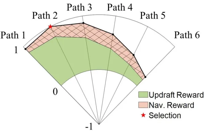
which is referred to as the reward pie. The updraft and navigation terms are represented in Fig.

3.2 as the green and red hatched areas respectively. The “spokes” on the pie chart represent the

six petals of the reduced ALFA flower. The reward is normalized by the maximum reward

value of the ALFA flower, allowing the reward values to stay between 1 and -1. As shown, the

updraft values begin at the center arc, representing zero, and the navigation values start where

the updraft values left off. The final reward values are represented with the bolded line, and

the red star indicates the selected path having the largest reward score. The reward pie is

31 Figure 3.2: The reward pie.

3.4 Navigation Baseline

The focus of this work is to determine whether this algorithm can enable the aircraft to harness

energy from the atmosphere. However, the ultimate goal of an aircraft mission is to reach the

waypoints and complete objectives. Using ALFA, the priority between reaching waypoints and

harnessing energy from updrafts can be adjusted to produce the flight behavior required for a

particular mission. The reward function priorities can be set such that the aircraft ignores all

updrafts and single-mindedly follows waypoints or only focuses on harnessing updrafts and

never reaching mission waypoints. Fig. 3.3 shows a flight conducted where the energy

harvesting ratio was set to heavily favor navigating to waypoints with a ratio of wU to wN of 1 to 5. The flight indicates that the aircraft flew directly to each waypoint with minimal

deviations from the straight path. The small sinusoidal motion observed along the flight path

is caused by the lack of a straight flight option in the ALFA flower as discussed previously.

32 following autopilot. From this point on, the updraft weight was increased so that the aircraft

was able to harvest energy. The remainder of this dissertation focuses on the behaviors

produced by the algorithm when set to harvest energy, and flights that harvest energy at the

expense of not reaching all waypoints are considered acceptable for analyzing the soaring

behavior produced.

Figure 3.3: Altitude and flight path while prioritizing navigation.

3.5 Illustrative Flight

The following flight case demonstrates the feasibility of ALFA. In this flight, the aircraft was

manually hand-launched, flown to an altitude of 170 meters, and then controlled by ALFA for

the remainder of the flight until landing. Fig. 3.4 shows the time variation of altitude for a

portion of an ALFA controlled flight. Fig. 3.5 shows the flight path over an image of the flight

field, and Fig. 3.6 shows a three-dimensional view of the flight path. The same color scale has

been used in all three figures. The aircraft’s mission is to fly a triangle between waypoints A,

B and C, and to exploit wind conditions whenever possible. The aircraft updates its waypoint

33 As shown in Figs. 3.4 to 3.6, to describe the ALFA behavior, the flight was divided

into four sections, separated by circled numbers. Section one (1 to 2) shows the aircraft gaining

altitude and circling in an updraft, as well as meandering between areas of good lift heading to

the first two waypoints. Waypoints are indicated by the white circles in Fig. 3.5. Section two

(2 to 3) shows an area where the aircraft exits the updraft to travel toward the next waypoint

and loiters in a weak area of lift. Section three (3 to 4) shows a period where there is almost no

updraft present, but the aircraft still searches the region for an updraft. In section four (4 to 5),

the aircraft has again found a good updraft and circles to gain altitude.

Figure 3.4: Altitude flight profile (color map represents aircraft altitude).

Table 3.1: Sink Rates for Illustrative Flight Sections (unassisted sink rate = 0.7 m/s).

Section 1 (m/s) -0.371

Section 2 (m/s) 0.359

Section 3 (m/s) 0.663

34 The constant exploitation of the small updrafts and wind variations while searching for

stronger updrafts allows the aircraft to fly at a reduced sink rate from that of a direct glide to

its destination. Herein ALFA’s potentially greatest benefit to soaring is demonstrated. For

comparison, the unassisted sink rate, which is the average sink rate along portions of the flight

where the aircraft glides unassisted by the algorithm, is 0.7 m/s. This value represents the

average sink rate of several flights that glided directly between these waypoints without using

power or ALFA to harness energy. Table 3.1 shows the average sink rates for the sections of

the flight path. In all the flight path sections, ALFA performed better than the unassisted sink

rate. In sections 1 and 4, the aircraft demonstrated a climb rate, which indicates the presence

of a strong updraft in the area and showed that ALFA was able to harvest energy from the

rising air successfully. Sections 2 and 3 brought the aircraft to a region of weaker updrafts

where it lost altitude, but still flew with a sink rate less than the unassisted sink rate.

35 While traveling toward waypoint A, the aircraft utilized updrafts and executed several

turns to remain in the favorable area of updraft. After reaching waypoint A, it started

meandering toward the second waypoint while staying in a favorable updraft. Near waypoint

B, the aircraft noticed a possible updraft south of the waypoint and executed three turns in the

updraft at that location. Then the navigation term gained priority over the updraft term and the

aircraft proceeded past waypoint B. Heading to waypoint C, the algorithm directed the aircraft

to loiter in an area of weaker updraft, and it stayed there slowly losing altitude until it reached

point 3. From point 3 to point 4, the updraft weakened or moved away, and the aircraft lost

altitude more rapidly. However, at point 4, the algorithm found another region of lift, and was

able to gain altitude by following the updraft and executing a couple of turns. After point 5,

the pilot took manual control and landed the aircraft. Throughout this flight, the aircraft never

reached waypoint C. While the ultimate goal for a soaring algorithm is to reach its objective

points while harvesting energy, the purpose of this work is to demonstrate the ability an aircraft

to harvest energy at all using the lumbered approach to autonomous soaring. So, while not

reaching waypoint C falls short of the ideal, this flight contains energy harvesting behaviors

that are valuable for this study.

36 As seen in Fig. 3.6, the flight section between points 1 and 2 shows circling behavior.

The aircraft appears to follow either a thermal that rose at an angle to the ground or one that

was moving along at some speed. Fig. 3.7 shows a detailed view of flight section 1. As seen in

this figure, the aircraft circled three times before moving toward the next waypoint and circling

again. Near the end of the climb, the updraft weakened to the point where the navigation term

of the reward function influenced the aircraft to begin heading toward the next objective point.

By this point, the aircraft had gained 85 meters in altitude and was heading toward the next

objective.

Figure 3.7: Detailed view on the 85-meter climb in section 1 (between points 1-2).

Throughout this flight, ALFA was able to identify and remain in areas of updraft. It

demonstrated an ability to meander and circle in a thermal. It was able to loiter in areas of a

weaker updraft, which allowed it to sink at a slower rate than the unassisted sink rate. With

ALFA, the endurance of the aircraft during this flight improved from an estimated total flight

time of 180 seconds associated with an unassisted glide, to 810 seconds, an improvement of

350%. The flight demonstrates the feasibility of using the lumbered approach for autonomous

37

Chapter 4

Detailed Flight Analysis

In this chapter, three flights that were selected to demonstrate the feasibility of ALFA

(see Figs. 4.1 and 4.2). Flight 1 was waypoint oriented, and showed the aircraft navigating the

airspace with minimal deviations from direct waypoint paths. While navigating between the

waypoints, the aircraft demonstrated a tendency to zigzag and avoid straight flight paths. In

flight 2, the aircraft’s waypoints were laid out in a triangle, but the aircraft prioritized updraft

exploitation over waypoint navigation. In this case, the aircraft was able to explore and gain

altitude, but only reached two of its three waypoints. In flight 3, the aircraft was given a loiter

command near a thermal, and ALFA was able to exploit energy from the thermal without

exploring too far from its loitering location.

Eight segments were selected from these three flights to demonstrate specific flight

behaviors produced by the algorithm (see Fig. 4.1). Before reviewing the individual flight

segments more closely in the next section, notice that the aircraft consistently performed better

with ALFA than when unassisted by the algorithm. Table 4.1 compares aircraft sink rates over

each of the flight segments and shows that the sink rate with ALFA was lower than the

unassisted sink rate of 0.7 m/s. Recall that this value represents the average sink rate of the

aircraft over several flights when set to navigate the waypoints while gliding, without using

the algorithm. Segment 2, which had the highest sink rate of the segments, still shows a sink

rate less than the unassisted sink rate. The best sink rates were actually climb rates, and these

38 ALFA exhibited great energy savings in addition to gaining energy from the classified

updrafts.

Table 4.1: Sink Rates for Detailed Flight Sections (unassisted sink rate = 0.7 m/s).

Segment 1 (m/s) 0.3

Segment 2 (m/s) 0.5

Segment 3 (m/s) 0.4

Segment 4 (m/s) -0.6

Segment 5 (m/s) -0.2

Segment 6 (m/s) -0.4

Segment 7 (m/s) -0.4

Segment 8 (m/s) -0.2

39 Figure 4.2: Aircraft flight paths.

4.1 Observed Behavior

The segments introduced above illustrate eight flight behaviors exhibited by the ALFA

controlled aircraft. ALFA flight behavior is made up of three simple behavior elements, a

circle, a straight line and a random line. These elements combine to produce various flight

behaviors, such as the eight behaviors identified below. Flight segment 1, Search and Return,

shows how the aircraft transitions from waypoint following to exploration behavior. In

segment 2, Circle Away, the aircraft executes several loops in response to the wind conditions.

In segment 3, Regional Loiter, the aircraft exhibits loitering behavior. In segment 4, Sine

Climb, it zigzags toward its waypoint while gaining altitude approaching a thermal updraft.

These four flight segments show how ALFA responds to rapidly changing, and often weaker,

unclassified updrafts, while demonstrating exploration behavior. In segment 5, Loiter, the

aircraft maintains and slowly increases its altitude while loitering near a point. In segment 6,

Thermal Loiter, the aircraft executes a nice circling pattern to gain altitude in a thermal.

40 8, Stationary Thermal, the aircraft circles to remain in a stationary thermal. These last four

segments illustrate how ALFA behaves near classi