A Bayesian Framework for Probabilistic Seismic Fragility Assessment of Structures.

(1)

ABSTRACT

TADINADA, SASHI KANTH. A Bayesian Framework for Probabilistic Seismic Fragility Assessment of Structures (Under the direction of Dr. Abhinav Gupta.)

A statistical framework is proposed to address the problem of evaluating and updating estimates of seismic fragility for structural systems in nuclear power plants and other critical infrastructure facilities. The main objective of the framework is to enable (i) integration of

fragility estimates from existing studies with the new fragility data from experiments or finite element simulations; (ii) planning and allocation of resources for efficient collection of

fragility data. Seismic fragility analyses of large-scale engineering structures is performed by conducting large-scale simulations involving multiple nonlinear time-history analyses using

experimentally-validated finite element models. Accurate estimation of fragility often demands a formidable number of nonlinear time-history simulations which can be computationally prohibitive. A computational methodology based on Bayesian inference

techniques is proposed to reduce the computational effort and efficient allocation of

computing resources. Application of the proposed methodology to large-scale piping systems

with localized nonlinearities is simplified further by proposing an equivalent linearization technique. A fragility model is developed for these systems where linearization of the localized nonlinearity enables us to evaluate a robust prior estimate of fragility using only

elastic time-history analyses. The model is incorporated into the Bayesian framework to evaluate posterior estimates by updating the prior using a much reduced number of nonlinear

time-history analyses. Modeling of uncertainties in the interdependencies between input parameters (material and model) is an important step in setting up probabilistic simulations. A sampling algorithm is suggested in order to facilitate simulation of closely-spaced random

(2)

(3)

A Bayesian Framework for Probabilistic Seismic Fragility Assessment of Structures

by

Sashi Kanth Tadinada

A thesis submitted to the Graduate Faculty of North Carolina State University

in partial fulfillment of the requirements for the Degree of

Doctor of Philosophy

Civil Engineering

Raleigh, North Carolina 2012

APPROVED BY:

Dr. Vernon Matzen Dr. Mervyn Kowalsky

Dr. Shamim Rahman Dr. Abhinav Gupta

(4)

ii

DEDICATION

(5)

iii

BIOGRAPHY

Sashi Kanth Tadinada was born on August 26th, 1983 in Kakinada, India. His family hails

from the town of Rajahmundry in India. He joined the undergraduate program in civil engineering at Indian Institute of Technology, Roorkee in July 2000 and received the Bachelors of Technology (B.Tech) degree in May 2004. Following graduation, he worked for

two years at Larsen & Toubro Ltd., - Engineering Construction and Contracts Division (L&T-ECCD) as a senior engineer in their Transportation Infrastructure (TI) Business Unit in

New Delhi, India. In August 2006, he came to the U.S. to join the graduate school pursuing both MS (2008) and PhD (2012) degrees from North Carolina State University.

Sashi’s research interests include structural dynamics, Bayesian statistics, probabilistic

(6)

iv

ACKNOWLEDGEMENTS

The research was supported by the Center for Nuclear Power Plant Structures, Equipment

and Piping at North Carolina State University. Resources for the center came from dues of the member organizations, National Science Foundation, Department of Civil, Construction and Environmental Engineering and College of Engineering at NCSU. I am greatly indebted

to the center for proving me with all the facilities and support throughout my graduate school. I would also like to thank all the staff members of the Civil Engineering department

for their help and support extended over the years.

I would like to express deepest and sincere gratitude for my advisor, Dr. Abhinav Gupta for giving me this opportunity to pursue my graduate studies and teaching me

everything about scientific research & writing. His constant guidance and inspiration throughout my research as well as in the preparation of this manuscript is simply invaluable.

I would like to thank Dr. Mervyn Kowalsky, Dr. Vernon Matzen and Dr. Shamim Rahman for graciously agreeing to serve on my doctoral committee and for their valuable suggestions. Special thanks to my colleagues and friends – Sami, Ju and Yonghee for sharing the results

from their work and for their constant input and feedback without which this collaborative research could not have been possible.

None of this effort would have been remotely possible without the unconditional love, support and encouragement from my dear parents and my kid brother. I appreciate the

(7)

v

friends I made during my stay at NCSU. Last but not the least, I want to thank the workshop “Medhajananam” and its creator Krishna Sharma for lending a unique and beautiful

(8)

vi

TABLE OF CONTENTS

LIST OF FIGURES ... ix

LIST OF TABLES ... xiii

PART 1: INTRODUCTION ... 1

1. Background ... 2

2. Structural Fragility ... 7

3. Bayesian Inference ... 14

4. Research Objectives ... 16

5. Proposed Research ... 17

6. Organization ... 23

References ... 24

PART II : A BAYESIAN FRAMEWORK FOR ESTIMATING AND UPDATING SEISMIC FRAGILITY OF STRUCTURES ... 26

1. Background ... 29

2. The Log-normal Fragility Model ... 34

3. Bayesian Framework for Updating Structural Fragility ... 38

4. Planning of Probabilistic Simulations ... 44

5. Conclusion ... 60

Acknowledgements ... 62

(9)

vii

PART III : STRUCTURAL FRAGILITY OF LARGE-SCALE PIPING SYSTEMS USING

EQUIVALENT ELASTIC TIME-HISTORY SIMULATIONS ... 75

1. Introduction ... 78

2. Bayesian Updating of Structural Fragility ... 85

3. Equivalent Linearization ... 90

4. Concept of Equivalent Elastic Limit State ... 93

5. Estimating the Equivalent Elastic Limit State ... 95

6. Application to Hospital Piping System Fragility ... 112

References ... 119

PART IV: SIMULATION OF CONSTRAINED, CLOSELY-SPACED RANDOM VARIABLES IN ENGINEERING RISK ANALYSES ... 137

1. Background ... 139

2. Sampling Random Variables with an Order Constraint ... 144

3. Application Examples ... 160

4. Extension to Other Constraints ... 162

References ... 168

(10)

viii

PART V: SUMMARY, CONCLUSIONS, AND RECOMMENDATIONS FOR FUTURE RESEARCH ... 198

(11)

ix

LIST OF FIGURES

PART II : A BAYESIAN FRAMEWORK FOR ESTIMATING AND UPDATING SEISMIC FRAGILITY OF STRUCTURES

Figure 1: Box-shaped Reinforced Concrete Shear Wall ... 67

Figure 2: Fragility Curve of the Box-type shear wall structure ... 68

Figure 3(a): Prior and Posterior densities of a~ ... 68

Figure 3(b): Prior and Posterior densities of _r ... 69

Figure 4: Comparison of prior and updated median fragility curves ... 70

Figure 5: 95% Confidence Bands on Prior and Posterior Fragility Curves ... 71

Figure 6: Convergence criteria as a function of q based on EPRI (1994) prior information ... 72

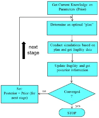
Figure 7: Flowchart for the Incremental Procedure of Planning and Conducting Probabilistic Simulations ... 73

Figure 8: Median Fragility Curves from Posterior Statistics at the End of Each Stage ... 74

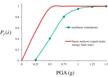
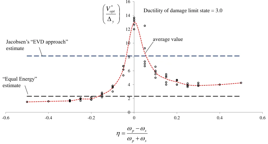
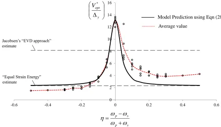
PART III : STRUCTURAL FRAGILITY OF LARGE-SCALE PIPING SYSTEMS USING EQUIVALENT ELASTIC TIME-HISTORY SIMULATIONS Figure 1: Representative Nonlinear and Equivalent Linear Systems ... 122

Figure 2: Force-Displacement Relationships for both Nonlinear and Linear Systems ... 122

(12)

x

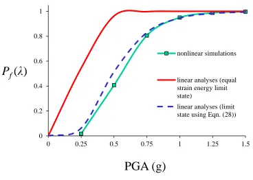
Figure 4: Representative Primary-Secondary Coupled System for the Illustrative Example ... 124 Figure 5: Seismic Fragility Curves from Nonlinear and Linear Time-History

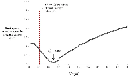
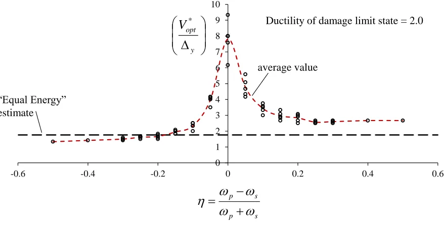
Simulations for the Example Structure ... 125 Figure 6: Error between fragility from elastic analyses and the actual fragility for the example structure ... 126 Figure 7: Effect of tuning between primary and secondary systems on the equivalent elastic limit state ... 127 Figure 8: Estimation of equivalent elastic limit state value using the equivalent viscous damping concept ... 128 Figure 9: Comparison of equivalent elastic limit states from simulations and

estimators (Failure Ductility = 2) ... 128 Figure 10: Comparison of equivalent elastic limit states from simulations and

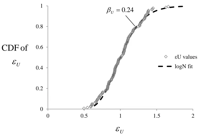
estimators (Failure Ductility = 3) ... 129 Figure 11: Validation of the model for damage ductility level = 2.0 ... 130 Figure 12: Validation of the model for damage ductility level = 3.0 ... 131 Figure 13: Seismic Fragility Curves from Nonlinear and Equivalent Linear Analyses for the Example Structure ... 132 Figure 14: Variations in _U ... 133 Figure 15: Hospital Main Piping System with a 2-inch Branch Containing the

(13)

xi

PART IV: SIMULATION OF CONSTRAINED, CLOSELY-SPACED RANDOM VARIABLES IN ENGINEERING RISK ANALYSES

Figure 1: Probability Density Functions of ₁and ₂ ... 181

Figure 2: Sample Space for f_U_,_V

 

u,v ... 182

Figure 3: Uniformly- Distributed Probability Density Functions of ₁and ₂ ... 182

Figure 4: Sample space of U-V Discretized as a Grid and the Properties of Constituent Grid Objects ... 183

Figure 5(a): Plot of f_U_,_V

 

u,v for Example Case 1 ... 184

Figure 5(b): Scatter plot of 1000 Samples



₁,₂



as Simulated (Case 1) ... 185

Figure 5(c): Comparison of Sampled Vs. Expected PDFs (Case 1) ... 186

Figure 6(a): Plot of fU,V

 

Figure 6(b): Scatter Plot of 1000 Samples



₁,₂



as Simulated (Example Case 2) ... 188

Figure 7(a): Plot of f_U_,_V

 

Figure 7(b): Scatter Plot of 1000 Samples



₁,₂



as Simulated (Example Case 3) ... 191

Figure 8: An 8 Storey Structural System ... 193

(14)

xii

Figure 10: Application to Other Constraints ... 195

Figure 11: f_U_,_V

 

u,v if Region R is a circle ... 196

Figure A-1: Convergence of the Algorithm in Example Case 1 ... 197

(15)

xiii

LIST OF TABLES

PART II : A BAYESIAN FRAMEWORK FOR ESTIMATING AND UPDATING SEISMIC FRAGILITY OF STRUCTURES

Table 1(a): Results of the Stage-wise Implementation of Probabilistic Simulations for Shear Wall Fragility ... 65 Table 1(b): Summary of the Stage-wise Implementation of Probabilistic Simulations ... 66

PART IV: SIMULATION OF CONSTRAINED, CLOSELY-SPACED RANDOM VARIABLES IN ENGINEERING RISK ANALYSES

(16)

1

PART I

(17)

2

1. BACKGROUND

1.1 Probabilistic Seismic Risk Analysis (PSRA)

The fundamental goal in the seismic design of any Nuclear Power Plant (NPP) is the minimization of radiological risk (release of radioactive emissions into the environment) and

ensuring the safety during and after an earthquake. It is critical that engineers be able to estimate the associated risks due to seismic events to a high degree of confidence. In the nuclear industry, this is achieved using a detailed probabilistic framework that carefully

accounts for uncertainties in the expected intensity of ground motions, the predicted response of the structures and ultimately, the chain of events that could lead to the catastrophic failure. The regulatory guide (USNRC, 1983) is a comprehensive document establishing a detailed

framework for Probabilistic Risk Analysis (PRA) of Nuclear Power Plants. It identifies the following analyses as key elements of seismic risk assessment for any nuclear power plant

structure:

 Seismic Hazard Analysis at the site – The seismic hazard H

 

 at a site describes the frequency i.e. the probability per year that an earthquake with a Peak Ground

Acceleration (PGA) value equal to is likely to occur. The seismic hazard H

 

 is usually determined from a probabilistic seismic hazard model that incorporates the

(18)

3

 The Responses of Plant Systems and Structures –In order to obtain the probability of damage given an earthquake of PGA level equal to , the statistical properties of the

seismic response of each structural system in the power plant need to be evaluated.  Component Fragilities – The fragility of a structural component P_f

 

 is defined as

the probability of exceedence that the component’s response will exceed a specified

limit-state when subjected to seismic excitation of PGA equal to . Specifying the limit-state or defining what constitutes performance criteria is a key step in evaluating

the component fragilities. The performance criteria are determined from typical failure modes and sequence of events that lead to the overall catastrophic failure.  Plant Systems and Accident Sequences – The constituent component fragilities are

used to evaluate the overall system-level fragility P_f_,_SYS

 

 based on initiating events, failure sequence and event-tree models which carefully consider all possibilities

leading to radiological release. The overall risk P_F of the structure can be determined as the convolution of seismic hazard H

 

 and the system fragility curve P_f_,_SYS

 

 as

 



 

 d

d dP H

PF f SYS

, 0





 (1)

 Consequence Analyses – Lastly, a consequence analysis is carried out to estimate the

(19)

4

of risk curves which plots the frequency of exceedence per reactor-year vs. the

number of fatalities (USNRC, 1983).

1.2 Seismic design criteria

Consistent with the PRA framework of USNRC (1983), ASCE (2005) specified the seismic

design criteria for nuclear power plant structures based on a Performance-Goal based (Risk Informed) approach. ASCE (2005) enumerates five different Seismic Design Categories (SDCs). The SDCs range from 1 for conventional buildings to 5 for critical facilities like

nuclear reactors. Additionally, four design limit states were also defined - Limit State A (“large permanent distortion for near-collapse conditions”) to Limit State D (“essentially

elastic behavior”). Each SDC has a target performance goal PF for any structure being

designed in that particular SDC. For example, PF = 1 x 10-5/yr for SDC – 5D implies that for

any structural design that belongs to Seismic Design Category 5 and failure Limit State D,

the overall seismic risk evaluated using Equation (1) cannot exceed the performance goal of

F

P = 1 x 10-5 /yr. In addition to the overall performance goal P_F , ASCE (2005) also prescribes that the structure must have sufficient levels of conservatism in form of minimum seismic margin factors Fp% such that the following probability goals are reasonably achieved:

1. Less than About a 1% Probability of Unacceptable Performance for the

(20)

5

2. Less than About a 10% Probability of Unacceptable Performance for a Ground Motion Equal to 150% of the Design Basis Earthquake (DBE)

Ground Motion

The seismic margin factor, Fp%is defined as a ratio of the PGA corresponding to the p%

probability of failure on the fragility curve to the PGA of the Design Basis Earthquake (DBE) as per Equation (2):

 

DBE p P_f p

% F

1 %



 (2)

where P_f

 

 is the fragility curve of the structure with respect to a specified limit state. From the above probability goals, all Structures, Systems and Components (SSC) designed

according to ASCE (2005) criteria must demonstrate seismic margin factors - F1% = 1.0 and

F10% = 1.5 corresponding to the “Unacceptable Performance” defined as the “onset of

significant inelastic deformation” limit state.

USNRC (2010) and USNRC (1993) prescribe an additional plant-level seismic margin by adopting risk-informed acceptance criteria for all New Standard Plant designs.

According to USNRC (1993), it is required that all new plant designs must demonstrate that the seismic margin corresponding to 1% probability of failure on “Core Damage” fragility

curve must be at least 1.67 i.e. F1% = 1.67. At this point, a distinction must be made between

the seismic margins prescribed by ASCE (2005) - F1% = 1.0 and USNRC (1993) - F1% = 1.67

(21)

6

limit states and different fragility curves altogether. The ASCE (2005) seismic margin factors F1% = 1.0 ; F10% = 1.5 pertain to the component-level fragilities for a limit-state characterized

as “onset of significant inelastic deformation” limit state whereas the USNRC (1993) seismic margin factor should be evaluated from a “Core Damage” plant-level fragility curve.

Kennedy (2007) argues that ASCE (2005) values of component-level seismic margins could be substantially too low as a design criteria for achieving the more stringent seismic margin criteria laid down by USNRC (1993). For this reason, USNRC (2001) adopted a component-level design seismic margins for the “Core Damage” limit state as F1% = 1.67 to be consistent

with the overriding evaluation criteria of USNRC (1993). Using the overall target

performance goal PF specifications, Kennedy (2007) presented a detailed discussion on the

risk-informed approach for establishing the design ground motion or the Site Specific Response Spectrum (SSRS) corresponding to the Safe Shutdown Earthquake (SSE) for future

nuclear plant designs defined on the basis of ASCE (2005) Standard.

In summary, the acceptability of seismic design for a NPP structure depends on

whether it satisfies the criteria in terms of Target Performance Goal PF corresponding to its

Seismic Design Category (SDC) and whether the design has sufficient “Core Damage”

seismic margin factor F1%. From Equations (1) and (2), it can be inferred that both the

quantities PF and F1% are evaluated from the overall system-level fragility curve, Pf,SYS

 



which in turn depends on the fragilities of individual components. A careful examination of

(22)

7

structural fragilities is one of most important and influential steps in the entire framework. Moreover, the minimum seismic margins such as F1% = 1.67 laid down by USNRC (1993)

necessitates that the fragility of NPP structures be evaluated with adequate accuracy especially in the low-probability (tail) region of the fragility curve.

In this research, we propose development of a comprehensive framework to

accurately evaluate the system-level seismic fragility of any structural system in a NPP. The framework aims to integrate existing approaches and results from probabilistic finite-element

simulations using innovative statistical inference techniques to better facilitate establishing the USNRC (1993) criteria of F1% = 1.67 for NPP structures. The next section discusses some

of the existing approaches in fragility analysis of structures and elaborates on the specific objectives of the proposed research.

2. STRUCTURAL FRAGILITY

2.1 Definition

Seismic structural fragility P_f

 

 is defined as the probability of a structure to attain or exceed a specified damage state G(.) at a given measure of ground motion intensity  e.g. Peak Ground Acceleration (PGA) or Spectral Acceleration (Sa) etc. Mathematically, it is

(23)

8

 

 P



G(.)0|



P_f (3)

where the damage state G() is function of the vector 



₁,₂..._k



where ₁,₂..._kare the random variables representing various material, modeling and loading uncertainties for

the structure. In its most simplistic form, the damage state G(.) is often described by a function of at least two variables as:

D C D C

G( , )  (4)

where C represents the capacity of the structure corresponding to the specified damage condition and D denotes response demand on the structure at a given ground motion intensity

. In this case, the fragility is

 

 P



CD0|



Pf (5)

The capacity C (or “Strength”) of a structure may be defined as a limit seismic load that the structure can endure before the specified damage occurs. It is typically evaluated from material properties and other strength parameters like compression strength, yield stress,

design code equations etc. The demand, D (or “Load”) at any given ground motion intensity  is a function of modeling and analysis variables like finite element models, ground motion

histories, damping, soil-structure interaction etc. In a seismic fragility analysis, Equation (5)

(24)

9

2.2 Log-normal model based on design factors of safety

The fragility P_f

 

 is commonly interpreted as being a cumulative distribution function for the structural acceleration capacity. Current state of practice in the nuclear industry (EPRI,

1994) considers that the acceleration capacity, A of a structure can be modeled as follows:

R U m a

A   (6)

where a_m is the median acceleration capacity of the structure and _R denotes the inherent randomness of the capacity about the median and _R denotes the uncertainty in our knowledge of the median capacity itself. The _R and _U are modeled as log-normally distributed random variables with a median of unity and log-standard deviations of _R and

U

 respectively. Kennedy et al. (1980) have derived the expression for a fragility curve

corresponding to a confidence level α as follows:

 

   

 

   



 _ _

       



R U m f

a P



 

 

1

ln

(7)

(25)

10

 

                     2 2 ln U R m f a P     (8)

Furthermore, Kennedy et al. (1980) simplified the fragility estimation by expressing the acceleration capacity A as a product of safety margin factors and the PGA of the design earthquake, _design:



Fi



design

A



 (9)

The various F_i represent various safety margin factors accounting for inherent conservatism in strength and uncertainty in various design variables like capacity, ground motion, damping, soil-structure interaction, modal combination, response spectrum, modeling etc.

EachF_i is characterized as a lognormal variable similar to that of Equation (6) with a median value of Fˆ and log-standard deviations _i _Ri and_Ui . Thus, the parameters for the fragility curve of Equation (5) i.e. a_m, _R and _U can be finally given by









    2 2 ; ˆ i U U i R R design i m F a      (10)

This model provides a quick heuristic estimate of seismic fragility of a structure that is

(26)

11

estimates thereby leading to wide confidence bands associated with the median fragility

curves.

In order to minimize the width of the confidence bands in the tail region, we need more fragility data. In such cases, many researchers have used experimental test results, empirical damage data, incremental dynamic analyses and numerical simulations to develop

sophisticated structural fragility models for a various kinds of structures. Shinozuka et al (2000) utilized bridge damage data from 1995 Kobe earthquake to estimate the parameters of

the lognormal fragility model using Maximum Likelihood Estimation (MLE) methods. Zentner (2010) used a similar approach to obtain the parameters for the fragility of a reactor

coolant system from numerical simulations. Serder and Polat (2006) used incremental dynamic analyses to develop capacity models for the mid-rise R/C frame buildings and suggested regression relationships between fragility parameters and the number of storeys in

the building. Carausu and Vulpe (1996) proposed a fragility estimation method for seismically isolated NPP structures by deriving bi-linear regression relationships using data

on input Peak Ground Velocity (PGV) values and maximum displacements of the isolation layer. Ramamoorthy et al (2006), Do-Eun et al (2008) and Huang et al (2010) etc. suggested developing complex probabilistic models for predicting the strengths ("Capacity") and

responses ("Demand") for a variety of reinforced concrete structural systems using experimental data and finite element model simulations. The above methods for direct

(27)

12

component level fragilities where experimental and damage data is abundantly available. But, in the SPRA framework where the system-level fragilities are of prime interest, the lack

of any meaningful quantity of experience data and high costs involved in conducting dynamic experiments for collecting fragility data on large-scale structural systems pose a

limitation in directly applying these existing approaches. For large systems, one way to estimate system-level fragilities is to use nonlinear time history analyses of an experimentally-validated full-scale Finite Element model of the entire system. A

Monte-Carlo simulation is typically implemented to account for various kinds of uncertainties in material, modeling and ground motion input variables.

2.3 Fragility using Monte-Carlo simulations

Availability of computational resources can enable us to evaluate the fragility functions within a simulation-based framework until additional experience or empirical data becomes

available. Monte-Carlo based fragility estimation appears quite straightforward as it involves performing a large number of multiple dynamic analyses for the structure adequately accounting for various uncertainties in the material, modeling and loading parameters. The

fragility curve can be generated by evaluating the probability of failure at different levels of

ground motion intensities -₁,₂,..._k using the expression in Equation (3):

 









n j k

n G G

P

P _j

j j j

j

f ; 0; 1...

| 0 (.) 1 |

0

(.)    

 





(28)

13

where 1(.) is the indicator function and n_j is number of simulations conducted at ground motion intensity _j. The k levels of ground motion intensities ₁,₂,..._k must be carefully chosen so as to be able to predict the complete nature of the fragility function satisfactorily.

If n_j is sufficiently large, the fragility P_f

 

 can be simply obtained by computing the ratio of the number of times a particular damage state (.)G has been attained by the structure to the total number of simulations, n_j.

The accuracy of the Monte-Carlo simulation approach depends entirely on two

variables: (i) the vector of PGA values, λ



₁,₂,..._k



T; (ii) the vector N



n₁,n₂,...n_k



T

where n_j denotes the number of time-history analyses performed at each PGA _j for j = 1, … ,k. Therefore in real-life structural fragility estimation, a trade-off must be made between

the required accuracy of the fragility estimates and the total number of analyses





 k

j j sim n N

1

that can be performed efficiently. For simple structural systems with a small number of Degrees of Freedoms (DOFs), performing a large number of multiple time history analyses

does not impose any serious constraint. However, for a large non-linear structural system with many DOFs, each time-history analysis may demand significant computational

resources.

(29)

14

estimate of fragility curves for the structure and then use limited time-history simulation data to update the fragility curves. The Bayesian Inference techniques are a popular and powerful tool to effectively integrate existing information or “prior knowledge” on the random parameters in the fragility model with “newly collected information” from the time-history

simulations in order to obtain the updated or “posterior” fragility curves. The next section introduces the Bayesian updating approach and discusses how it can be used to update the

random parameters in fragility models.

3. BAYESIAN INFERENCE

Suppose that the structural fragility model P_f

 

 depends on a vector of random variables





T

.... , 2 1 





Θ such thatP_f

 

  f



;Θ



. Also assume that our current knowledge of Θ can

be represented by a joint density function - fΘ'



₁,₂...



. This



1, 2...



'  

Θ

f is often referred to as “prior” information and is generally obtained from professional knowledge of experts, past

studies etc. Suppose a vector of m observations - y



y₁,y₂...y_m



Tof structural fragility data have been collected. The Bayes Theorem can then be used to update our knowledge of the

random parameters using the observed data y to obtain the “posterior” information



y



Θ 1, 2...| '

'  

(30)

15







_{ }

 



 













_



 



 Θ y y y y y y Θ Θ Θ Θ d f P P E P P f P f ... , | ... , | ... , ... , | ... , | ... , 2 1 ' 2 1 2 1 2 1 ' 2 1 2 1 ' '             (12)

In Equation (12), P



₁,₂...|y



is often referred to as the “Likelihood function” of the random parameters. The integrations involved in the evaluation of P

 

y can be quite formidable to be evaluated by even numerical techniques especially for higher-order Θ. So,

the posterior statistics f_Θ''



₁,₂...|y



are typically computed by numerically generating a large number of posterior samples employing a special class of computational algorithms

called Markov Chain Monte Carlo (MCMC) methods (Winkler, 2003; Congdon, 2006).

Bayesian methods provide the flexibility to incorporate different types of data (experimental, empirical, numerical simulations, etc.) into a single fragility model and help reduce the

variability that might otherwise exist in predicted values due to limited data. A detailed updating procedure is illustrated in which we start with the initial fragility estimates based on

the conventional lognormal approach of Section 2.2 as "prior" information and then use the results from the time-history analyses of an experimentally-validated FE model to update the fragility curves based on Equation (12). Another advantage of the Bayesian inference

techniques is that they can be instrumental in optimizing the number of time history analyses required as well as the region of PGA values in which to conduct the time history analyses. Instead of performing an arbitrary number of time history analyses at various levels of PGAs,

(31)

16

posterior statistics as to how many more observations might be necessary to achieve specified convergence criterion. While studies like Hamada et al (2008) discuss methods

based on Genetic Algorithms (GA) to plan for reliability data collection, no explicit planning approach exists for conducting time history analyses and design of Monte-Carlo experiments

in structural fragility applications. A comprehensive methodology for a Bayesian statistics based planning of the Monte-Carlo simulations is also presented for reducing the total

computational effort involved.

4. RESEARCH OBJECTIVES

The primary objective of this research is to develop a comprehensive framework for evaluating seismic fragilities for large-scale structural systems as well as updating them

based on the availability of additional fragility data. The key aspects desired in the proposed framework are:

 The framework should be able to predict the structural fragility estimates to desired

limits of accuracy with a high degree of confidence.

 The framework must aim to reduce the total number of nonlinear time history

analyses required for a specified degree of accuracy in the fragility curve.

 The framework should be robust enough to account for uncertainties in complex

(32)

17

5. PROPOSED RESEARCH

The specific tasks needed to accomplish the objectives of this research can be characterized

in the following sub-sections:

5.1 Evaluate the limitations of existing approaches for evaluating structural fragility

 Study the current framework of the Seismic Probabilistic Risk Assessment (SPRA) in

the nuclear industry (Kennedy, 2007) Demonstrate the conventional approach of structural fragility calculation with the lognormal model based on design factors of

safety (EPRI, 1994) using an example of a Box-Shaped reinforced concrete shear wall. The purpose of this exercise is to determine if the existing approach yields

structural fragility estimates with sufficient degree of confidence required to establish the USNRC (1993) criteria.

 Stipulate maximum acceptable value for width of the 95% confidence bands as an

indicator of the level of the accuracy desired.

 Identify the limitations of the conventional approach:

o Relies on expert judgment and professional experience independent of the

specific design of a structural system

o The resultant fragility curves tend to be very sensitive to the

(33)

18

o No procedure exists to update fragility or reduce confidence bands using

additionally available data

5.2 Development of a Bayesian framework for updating structural fragility

System level fragilities are often calculated by a Monte-Carlo simulation in which the

experimentally validated finite element model of one or more components is incorporated into a system-level FE model. The non-linear large-scale system level model is then used to conduct multiple time history analyses within a Monte-Carlo framework to evaluate

system-level fragilities. The excessive computational time needed in conducting a single time history analysis renders this framework impractical if many different earthquake input motions are considered in the fragility evaluation. A Bayesian framework can be used quite effectively to

determine the number of time history simulations needed in order to achieve a desired degree of accuracy. Specific tasks in such a framework can be enumerated as:

 Determine the parameters associated with the fragility curve assuming the

conventional lognormal fragility model from the EPRI (1994) approach or any other

existing method. The prior information on the random parameters of the model - median capacity and the log-standard deviation must be specified based on this preliminary fragility analysis.

 Conduct a relatively small number of time-history analyses of the

(34)

19

 From the responses of each time history analysis at a given PGA, determine if the

structure has exceeded the specified limit state. Consider that the structure has

"failed" if the maximum responses from the analysis exceed the specified limit state.

 Using the entire failure data collected above, determine the "likelihood" function of

the random parameters of the lognormal model.

 Evaluate the "posterior" statistics of the random parameters - median capacity and the

log-standard deviation, from the "prior" fragility and the "likelihood" functions

employing the Bayes Theorem using Markov Chain Monte Carlo methods.

 Use the posterior statistics to compute the median fragility curve and the widths of the

associated 95% confidence bands. If the 95% confidence bands do not satisfy the specified convergence criteria, more simulations may be needed.

 In order to minimize the total number of time history analyses required for

convergence, an optimal plan for the Monte-Carlo simulation may be effective compared to conducting an arbitrary number of time history analyses at various levels

of PGA. It is proposed to develop such a plan based on Bayesian Inference and Markov Chain Monte Carlo methods.

5.3 Simulation of constrained, closely-spaced random variables in engineering risk analyses

Any Monte-Carlo simulation involving a large-scale structure needs to account for

(35)

20

variables. In such cases, care must be taken to accommodate these constraints while generating random sample sets of input variables for time history analyses. Consequently, we

need a sampling technique to generate sets of random variables so that they may be: (a) characterized by a continuous Probability Density Function (pdf); (b) subject to a non-linear

constraint. The various steps for achieving this objective are outlined below:

 Illustrate the limitations associated with ignoring the constraints between the input

parameters of a structure in a Monte-Carlo simulation. For example, closely-spaced

natural frequencies of a structure with the constraint that a simulated set of natural frequencies must always be an ordered set. Sampling of closely-spaced frequencies as

independent random variables may violate this constraint.

 Evaluate if simply rejecting the disordered or incorrect sets is an acceptable solution

to the above problem. This can be verified by comparing the shapes of the simulated

density functions with the expected distributions. If the overlap between the pdfs is significant, rejecting the improper sets may lead to considerable bias.

 Establish if using the explicit correlation coefficients can resolve the problem of

disordered/incorrect sampling.

 Evaluate the possibility of deriving an analytical solution from basic probability

(36)

21

 If an analytical solution is not possible, suggest a numerical procedure to obtain a

joint probability density function surface that can be used to the sample

closely-spaced constrained random-variables.

5.4 A Bayesian model for large-scale piping systems based on equivalent linear analyses

Sometimes, the fragility of certain structural systems which exhibit predominantly elastic deformations is often dictated by localized non-linearity present in connections and joints within the system. Typical examples include connections in piping systems of a nuclear

power plant or a hospital where the failures of T-Joints and/or bracing members often lead to the damage of the piping system. To evaluate the seismic fragility in such situations, the conventional EPRI (1994) approach to obtain the “prior” fragility curve cannot be

implemented directly and tends to suffer from lack of sufficient information. In this section, we propose a method to obtain improved estimates of “prior” fragility by conducting

multiple linear history analyses of an equivalent linear system. The use of linear time-history analyses to estimate the prior information has two distinct advantages:

(i) For any system with predominantly linear behavior, equivalent linearization of localized nonlinearities can lead to system fragilities that are quite close to the fragility that may be evaluated from multiple non-linear analyses. Therefore, this

(37)

22

(ii) The time-history response of a linear system at any PGA can be obtained by scaling the responses of the system calculated for a unit PGA case. The total

computational effort can therefore be minimized as only a set of elastic responses at a single PGA value are needed for computing the complete fragility curve.

Specific tasks needed to implement the proposed method are:

 Study the applicability of existing equivalent linearization techniques to large scale

piping systems. Identify the chief limitation(s) of extending the approach to such

systems.

 Introduce the concept of equivalent linear limit state: for a fragility curve of a

nonlinear system given by P_fNL

 

 P



G(.)0



, determine an equivalent linear limit state, Glin(.)corresponding to the actual limit state G(.) such that fragility evaluated from using the equivalent linearized system - P_flin

 

 P



Glin(.)0



is close to

 

 NL f P .

 Perform an exhaustive set of numerical simulations using representative systems to

propose general guidelines on evaluating Glin(.)as a function of structural properties and the desired limit state G(.)

 Incorporate the calculated prior P_flin

 

 based on _Glin(.)

into the generalized Bayesian

(38)

23

6. ORGANIZATION

This dissertation consists primarily of three manuscripts which will be submitted for

possible publications in peer reviewed journals. The first manuscript, Part II of the dissertation, presents the Bayesian statistical framework for seismic fragility evaluation of structures. The various features of the framework are illustrated using a detailed fragility

analysis of a Reinforced Concrete (RC) box-shaped shear wall. The second manuscript in this dissertation, Part III, discusses the evaluation of seismic fragility of nonlinear connections in

large piping systems using equivalent linearization techniques. The third manuscript in this dissertation, Part IV, addresses the problem of sampling closely-spaced random variables

subjected to inequality constraints for engineering risk analysis applications. Part V of this dissertation gives a summary and conclusions of this research and the anticipated future

(39)

24

REFERENCES

ASCE/SEI 43-05, "Seismic Design Criteria for Structures, Systems, and Components in Nuclear Facilities," American Society of Civil Engineers and Structural Engineering Institute, 2005.

Carausu, A. and Vulpe, A. “Fragility estimation for seismically isolated nuclear structures by high confidence low probability of failure values and bi-linear regression,” Nuclear Engineering and Design, 160 p. 287-297, 1996.

Congdon, P., “Bayesian Statistical Modelling,” Wiley Series in Probability and Statistics, 2nd Edition, 2006.

Do-Eun C., Gardoni, P., Rosowsky, D., Haukaas, T., “Probabilistic capacity models and seismic fragility estimates for RC columns subject to corrosion”, Reliability Engineering and System Safety, v 93, n 3, p 383-93, 2008

Electric Power Research Institute (EPRI), “Methodology for Developing Seismic Fragilities”, EPRI TR-103959 (Principal Investigators: Reed, J.W. and Kennedy, R.P.), Electric Power Research Institute, Palo Alto, California, 1994.

Hamada, M.S., Wilson, A., Reese, C. S., Martz, H., “Bayesian Reliability,” Springer Series in Statistics, 2008.

Huang, Q. Gardoni, P., Hurlebaus, S., “Probabilistic seismic demand models and fragility estimates for reinforced concrete highway bridges with one single-column bent,” Journal of Engineering Mechanics, v 136, n 11, p 1340-1353, 2010.

Kennedy, R.P., “Performance-Goal Based (Risk Informed) Approach for Establishing the SSE Site Specific Response Spectrum for Future Nuclear Power Plants,” Jaeger Lecture, SMIRT-19, Toronto, Canada, 2007.

Kennedy, R.P., Cornell, C.A., Campbell, R.D., Kaplan, S., Perla, H.F., “Probabilistic seismic safety of an existing nuclear power plant,” Nuclear Engineering and Design, 59, 315–338, 1980.

Petelet M., Iooss B., Asserin O., Loredo A., “Latin hypercube sampling with inequality constraints,” Advances in Statistical Analysis, submitted. Available at: http://hal.archives-ouvertes.fr/docs/00/52/00/21/PDF/AStA10_iooss_rev2.pdf, 2010.

(40)

25

Serdar K.M., Polat, Z., “Fragility analysis of mid-rise R/C frame buildings,” Engineering Structures, v 28, n 9, p 1335-1345, 2006.

Shinozuka, M., Feng, M.Q., Lee, J., Naganuma, “Statistical analysis of fragility curves,” Journal of Engineering Mechanics, v 126, n 12, p 1224-1231, 2000.

Tadinada S.K., “Consideration of Uncertainties in Seismic Analysis of Non-classically damped coupled systems,” Master’s Thesis, North Carolina State University, Available at:

http://repository.lib.ncsu.edu/ir/bitstream/1840.16/2134/1/etd.pdf , 2009.

USNRC, “PRA Procedures Guide: A Guide to the Performance of Probabilistic Risk Assessments for Nuclear Power Plants,” NUREG/CR-2300, 1983.

USNRC, “Policy, Technical, and Licensing Issues Pertaining to Evolutionary and Advanced Light-Water Reactor (ALWR) Designs, (Item II Q),” SECY-93-087, 1993.

USNRC, “Technical Basis for Revision of Regulatory Guidance on Design Ground Motions: Harzard- and Risk- Consistent Ground Motion Spectra Guidelines,” NUREG/CR-6728, 2001.

USNRC, “Interim Staff Guidance on Implementation of a Probabilistic Risk Assessment-Based Seismic Margin Analysis for New Reactors,” DC/COL-ISG-020, 2010.

Winkler, R.P., “An Introduction to Bayesian Inference and Decision,” Probabilistic Publishing, 2nd edition, 2003.

(41)

26

PART II

A BAYESIAN FRAMEWORK FOR ESTIMATING AND UPDATING SEISMIC FRAGILITY OF STRUCTURES

Sashi Kanth Tadinada and Abhinav Gupta

(42)

27

ABSTRACT

The fundamental goal in the seismic design of any Nuclear Power Plant (NPP) is the

minimization of radiological risk (release of radioactive emissions into the environment) and ensuring the operational safety immediately following an earthquake. It is therefore, critical that engineers be able to estimate the associated risks due to seismic events to a high degree

of confidence. In the nuclear industry, this is done using a detailed probabilistic framework that carefully accounts for all possible uncertainties in the expected intensity of ground

motions, the predicted response of the structures and ultimately, the chain of events that could lead to the catastrophic failure. For real-life complex systems with non-standard

designs, one realistic way of estimating seismic risk of the system is to use a robust experimentally-validated Finite-Element (FE) simulation model and perform multiple dynamic analyses by considering uncertainties in material, modeling and loading variables.

But this Probabilistic approach to seismic risk estimation has one important drawback - it requires a large number of computationally intensive simulations to be performed for

accurate estimates of risk. Typically, this demands for a trade-off between the desired accuracy of the risk estimates and the total number of simulations that can be performed in a reasonable time.

In this work, we present a comprehensive statistical framework based on Bayesian inference

(43)

28

(FE) simulations for seismic risk assessment of large-scale engineering structures. The salient features of the framework are:

a. Using Bayesian Inference to flexibly combine preliminary risk data from a variety of information sources like experiments, existing studies or simplified approaches with

data from FE simulations thus reducing the overall dependence on simulation data alone;

b. Embedding Bayesian methods within a stochastic optimization environment to help forecast, plan and allocate adequate computing resources such that the desired accuracy is achieved using minimum possible number of simulations.

(44)

29

1. BACKGROUND

Evaluation of seismic fragilities for structural systems is a key step in the Seismic

Probabilistic Risk Analysis (SPRA) of a Nuclear Power Plant (NPP). In the SPRA framework, a fragility curve describes the relationship between a ground motion intensity parameter like Peak Ground Acceleration (PGA) and the corresponding probability of failure

for specified performance criteria.

The widely used approach to evaluate structural fragilities in the nuclear industry is

the lognormal model based on design factors of safety (Kennedy et al, 1980; EPRI, 1994) which assumes a lognormal distribution for the acceleration capacity of the structure. USNRC (1993) has adopted a risk-informed acceptance criteria for new plant designs which

requires that all designs must demonstrate a safety factor of 1.67 over the 1% probability of failure (F1%) on the core damage fragility curve i.e. the probability of core damage in any

NPP should be less than 1% in the event of an earthquake whose PGA is 1.67 times the design basis level (Kennedy, 2007). Such a criterion necessitates that fragility of nuclear power plant structures be determined with adequate accuracy especially in low probability

regions (tail) of the fragility curve. However, the conventional EPRI (1994) approach relies heavily on data from past studies and expert judgment which may not always be available for

(45)

30

generally conservative leading to a wide band of confidence intervals for the median fragility

curve and consequently, greater variability in the fragility estimates.

In order to minimize the width of the confidence bands in the tail region, we need to acquire additional fragility data. In such cases, many researchers use experimental test results, empirical damage data, incremental dynamic analyses and numerical simulations to

develop sophisticated structural fragility models. Shinozuka et al (2000) utilized bridge damage data from 1995 Kobe earthquake to estimate the parameters of the lognormal

fragility model using Maximum Likelihood Estimation (MLE) methods. Zentner (2010) used likelihood estimation methods to obtain the parameters for the fragility of a reactor coolant

system from numerical simulation data. Kircil and Polat (2006) used incremental dynamic analyses to develop capacity models for the mid-rise Reinforced Concrete frame buildings and suggested regression relationships between fragility parameters and the number of

storeys in the building. Carausu and Vulpe (1996) proposed a fragility estimation method for seismically isolated NPP structures by deriving bi-linear regression relationship using data on

input Peak Ground Velocity (PGV) values and maximum displacements of the isolation layer. Mehrdad and Der Kiureghian (2001), Ramamoorthy et al (2006), Choe et al (2008) and Huang et al (2010) etc. suggested developing complex probabilistic models for predicting

the strengths ("Capacity") and responses ("Demand") for a variety of reinforced concrete structural systems using experimental data and finite element simulations. These methods for

(46)

31

component level fragilities where experimental and field data is abundant. However in the SPRA framework, it is the system-level fragilities of large structural systems that are of

prime interest. Experimental testing for fragility data on large scale systems in most cases is uneconomical and impractical thereby limiting the amount of data that can be collected.

Moreover, the fragility models at the component-level cannot always be extended in a straight-forward manner to the system level (Shinozuka et al, 2000). The system-fragility is typically determined from the constituent component fragilities using event and fault tree

models which consider the failure of a component as an independent event. However, seismic behavior of large-scale structural systems depends significantly on the dynamic

interactions between the sub-systems. The dynamic interaction effects cannot be considered in a fault- and event-tree based system reliability approach.

For large structural systems, a generally used approach for computing structural

fragility is to use probabilistic simulations involving multiple time history analyses of an experimentally validated Finite Element (FE) model of the structure (Komura et al, 1989;

Shinozuka and Kishimoto, 1989; Garcia and Soong, 2003). In this approach, the structural properties of the individual components and their failure mechanisms are studied in detail through careful testing. The validated models are then integrated into the large-scale finite

element model of the complete system. This approach allows for consideration of uncertainties in the physical variables, modeling nonlinearities, inter-dependencies between

(47)

32

history analyses are conducted at various levels of PGA to evaluate the fragility values. An important drawback of this approach is that it requires a large number of dynamic analyses to

accurately predict fragility in the low-probability region which can be highly inefficient and computationally prohibitive. Thus, a trade-off exists between the required accuracy of the

fragility estimates and the total number of analyses that can be completed in a reasonable manner.

To reduce the total number of time history analyses required, it is sometimes practical

to use conventional or existing approaches to derive preliminary estimates of fragility curves for the structure and then use simulation data from the time history analyses to update the

fragility curves as per desired accuracy. In this paper, we propose a framework based on Bayesian Inference techniques to update preliminary estimates of the fragility curves and reduce the width of the confidence bands associated with them. The purpose is to improve

the confidence in establishing the USNRC specified criteria of F1% = 1.67 mentioned earlier.

Bayesian Inference is a powerful statistical technique to combine existing or "prior"

knowledge with newly available data for improving the process of generating additional data.

A number of researchers have applied Bayesian techniques to address structural fragility problems. Gardoni et al (2002) presented a Bayesian framework to develop

multi-variate probabilistic capacity and demand models and applied it to Reinforced concrete bridge components. Straub and Der Kiureghian (2008) employed Bayesian methods to

(48)

33

dependence between empirical observations of seismic performance. Koursourelakis (2010) suggested a Bayesian framework to develop fragility surfaces simultaneously considering

four different ground motion intensity parameters instead of just the PGA and applied it to geotechnical problems. Many other researchers have used Bayesian approaches to update and

develop the probabilistic capacity and demand models using experimental data or time history analyses for a variety of structural systems such as Reinforced Concrete (RC) structural walls (Mehrdad and Der Kiureghian, 2001), RC bridge components (Gardoni et al,

2002; Zhong et al, 2009), RC frames (Ramamoorthy et al, 2008), woodframe structures (Pei et al, 2009), power plant equipment (Yuichi et al, 2005), multi-storey buildings (Bai et al,

2011) and so on. A common theme in all these studies is that the availability of additional data is used to update the median fragility curve. In this paper, we illustrate that while a median fragility curve can converge with the availability of only limited additional data, the

corresponding confidence bands associated with aleotary uncertainties can be significantly large. This means that accurate evaluation of a design parameter such as F1% with respect to

an acceptable criterion may require much more data.

Bayesian methods provide the flexibility to incorporate different types of data (experimental, empirical, numerical etc.) into a single fragility model and to draw reliable

inferences even with limited data. We present a procedure in which we start with the initial fragility estimates based on the conventional lognormal approach (EPRI, 1994) as "prior"

(49)

34

at various PGA levels are used to evaluate the updated or "posterior" fragility curves. It is illustrated that the Bayesian framework, even with a relatively small number of time-history

analyses data, is quite effective in achieving the convergence criteria. Another advantage of the Bayesian Inference technique is that it can be effective in reducing the number of time

history analyses required as well as identifying the region of PGA values in which to conduct the time history analyses. Instead of performing an arbitrary number of time history analyses at various levels of PGAs, one can start with a relatively small number of time history

analyses and infer from the posterior statistics as to how many more observations might be necessary to satisfy a specified convergence criterion. The advantages of the proposed

framework are illustrated by evaluating the seismic fragility of Reinforced Concrete (RC) Box-shaped shear wall.

2. THE LOG-NORMAL FRAGILITY MODEL

Current state-of-practice in the nuclear industry (Reed and Kennedy, 1994; EPRI, 1994)

considers that the acceleration capacity A of a structure can be modeled as a random variable:

R U m a

A   (1)

where a_m is the median acceleration capacity of the structure and _R is the random variable denoting the inherent randomness of the capacity about the median and the random variable

R

(50)

35

are modeled using the log-normal distribution with a median of unity and log-standard

deviations of _R and _U respectively. Using the relationship in Equation (1), the expression for the fragility curve corresponding to a confidence level α is given by Kennedy et al. (1980) as follows:

 

            _ _          R U m f a P      1 ln (2)

The median fragility curve can be written as

 

                     2 2 ln U R m f a P     (3)

In order to determine the parameters of the model, Kennedy et al. (1980) expressed

the acceleration capacity, A as a product of safety margin factors and the design level PGA -

design  :



Fi



design

A



 (4)

The various F_i ’s represent different safety margin factors accounting for

conservatism and uncertainty in the design variables like capacity, ground motion, damping,

(51)

36

itself characterized as a log-normal variable with a median value of Fˆ_i and its corresponding logarithmic-standard deviations _Ri and_Ui . Thus, the parameters for the fragility curve of Equation (2) i.e. a_m, _R and _U can be evaluated as:









 

 

2 2

; ˆ

i U U

i R R

design i

m F

a

 



(5)

2.1 Example –Reinforced Concrete box-type shear wall

The structural fragility of a Reinforced Concrete Box-shaped shear wall shown in Figure 1 is calculated using the EPRI (1994) approach. It is desired to evaluate the seismic fragility of this structure subjected to unidirectional earthquake excitations. For brevity, the detailed

calculations involved in evaluation of the various safety margin factors and their log-standard

deviations - Fˆ_i, _Ri and _Ui are not presented. The parameters of the resultant lognormal fragility curve were determined for the shear wall are determined as: a_m 1.658g ,

288 . 0 

R

 and _U 0.265.

Figure 2 gives the median fragility curve P_f

 

 calculated using Equation (3) and the corresponding 90% confidence bands based on Equation (2). It is evident from Figure 2 that the EPRI (1994) approach results in large confidence intervals associated with the median

fragility curves. This can be also be seen by examining the width of the 90% confidence

(52)

37

value of a_m can lie anywhere between 0.99g and 2.78g with a probability of 90%. One reason for such a conservatism in the fragility estimates is that the values of the safety

factors, Fˆ_i, _Ri and _Ui are based on capacity equations from design codes, expert judgment and existing professional experience pertaining to typical design practices in the industry.

One direct way to overcome the wide confidence bands of the fragility curves from the EPRI (1994) approach is to estimate fragility from the results of nonlinear seismic analysis of the structure using an experimentally validated Finite Element (FE) model by

considering uncertainties in material, modeling and loading variables. But this approach to risk estimation has one important drawback - it requires a large number of simulations to be

performed for accurate estimates of risk. This can be a limitation in the case of large FE models which often take significant computational time even for a single analysis. Therefore, a trade-off is often required between the desired accuracy of the risk estimates and the total

number of analyses that can be performed in a reasonable time.

2.2 Objective

The primary objective of this study is to develop a comprehensive framework for evaluating system-level structural fragilities as well as updating them based on the availability of

additional fragility data. The key aspects desired in the proposed framework are:

 The framework should be able to predict the structural fragility estimates to desired

(53)

38

 The framework should be capable of considering the effects of various kinds of

uncertainties on the seismic response of the structure

 The framework must aim to reduce the total number of nonlinear time history

analyses required for a specified degree of accuracy in the fragility curve.

The proposed framework implements Bayesian inference techniques in order to evaluate the seismic fragilities. To minimize the total computational effort, the framework

updates the initial fragility curves obtained from the conventional (EPRI, 1994) approach (called “prior fragility”) using the data from time history simulations to develop fragility

curves of large-scale systems with an intent to achieve relatively much narrower confidence bands. The next section introduces the Bayesian updating approach and discusses how one

can implement it to update the fragility curves when new information becomes available.

3. BAYESIAN FRAMEWORK FOR UPDATING STRUCTURAL FRAGILITY

3.1 Bayesian inference

In general, any structural fragility model can be represented as a function of the earthquake

intensity , i.e. P_f