Performance Analysis of Dynamic Source Routing Protocol for
Ad Hoc Networks Based on Taguchi’s Method
1
Muhammad Hisyam Lee,2Mazalan Sarahintu
Faculty of Science, Universiti Teknologi Malaysia, 81310 Skudai, Johor, Malaysia e-mail:1
m381 [email protected]
Abstract Mobile Ad Hoc Networks (MANET) are self-organizing, multi-hop wireless networks. The MANETs are rapidly deplorable due to the absence of a fixed infrastruc-ture. A number of routing protocols have been proposed in solving routing problems for this type of network, to provide and maintain better connectivity in the network. Before being implemented in real life, the performance of a routing protocol is eval-uated primarily through the simulation experiments. This paper presents Taguchi’s method to optimize networks parameters of dynamic source routing protocol for such mentioned networks. Performance analysis of the drop rate are conducted based on three factors namely terrain size, pause time, and node velocity. An L4 orthogonal array was used to design the experiment. The study indicated that, among the factors considered, terrain was found to have strongest effects, followed by pause time. By taking into consideration factorial effects, the optimal levels were found to beA1,B1, and C1, corresponding to terrain size of 25 ×25 m
2
, pause time of 15 seconds, and node velocity of 0.72 m/s. Using these factor-levels combination, a minimum of 3.26% drop rate can be obtained.
Keywords Taguchi method; parameter optimization; performance evaluation; ad hoc network; dynamic source routing protocol.
1
Introduction
An ad hoc network is a special type of wireless mobile networks, in which a collection of mobile platforms such as PDAs, cell-phones, and laptops, which are also known as nodes, formed a temporary network without relying on any organized administration, such as base station [2]. This network is useful in disaster recovery situations and places with non-existing or damaged communication infrastructure, where a rapid deployment of a communication network is needed. An ad hoc network is also useful in conferences, where people in a conference can form a temporary network without engaging the services of pre-existing network, for example wireless LANs.
the goal of the routing protocol is to dynamically establish and maintain routing in the network, forwarding packets for each other to allow communication between nodes not directly within wireless transmission range. Until now, there are no standard for the routing protocol for mobile ad hoc networks.
A number of routing protocols have been proposed in solving routing problems for mobile ad hoc networks [17], utilizing a variety of different algorithms and approaches, one of which is DSR, a reactive routing protocol. The main feature of this routing protocol is that routes are created when needed. (To know how the DSR operates please refer to [1, 2]). In order to know how well the DSR performs in a certain situation, for example where nodes are highly mobile, the performance of the routing protocol is measured primarily through simulation experiments (see [2, 4, 5, 12, 13, 16]). In these experiments, the performance of the DSR protocol is evaluated by looking at some performance metrics, for example routing overhead, where the lower the routing overhead, the better the DSR protocol in terms of consuming energy [16].
In practice, the performance of the DSR can be influenced by several factors, including terrain size, pause time, and node velocity [12]. Pause time and node velocity can cause link failures, which negatively impact routing and quality of service supports [14]. Terrain size has a considerable impact on the network scalability, that is the number of nodes in the network that can be scaled [15].
Considering the facts mentioned above leads to some questions: what is the most sig-nificant factor affecting certain performance metric of the DSR? What are the ranks of the factors? What is the best combination of factor levels (values) that reliable to provide a good response metrics for the DSR? The above mentioned questions may need to be answered due to some beneficial results. For example, suppose pause time (node mobility) is shown to have a greater impact on a performance metric of the DSR protocol than any factors. Therefore, if there is an attempt to obtain better performance of the DSR protocol with respect to the metric, something should be done with the node mobility, for example the current model utilizing pause time (i.e., random way point model) is improved or changed with another model. Another benefit, the combinations of factor-levels that would suggest here might be used as a reference of factor settings to evaluate performance of any routing protocol when considered a scenario taken from life (either small or moderate border sizes and density).
In particular, this work aims to estimate the impacts of network factors on the perfor-mance of the DSR with respect to a perforperfor-mance metric, namely drop rate. Taguchi method is presented to achieve the aim. The remainder of this paper is organized as follows. In section 2, we discuss the introduction to Taguchi method. In section 3, we discuss the ex-perimental setup. In section 4, we present our analysis and discussions. Finally, in section 5, we conclude our results.
2
Methods
There are many ways to design an experiment, but the most frequently used approach is a full factorial experiment. However, for full factorial experiments, there are 2k
possible trials that must be conducted (k= the number of factors each at two levels). Therefore, it is very time consuming when many factors are considered [8].
experiments (FFEs) were developed. FFEs use only a portion of the total possible combi-nations to estimate the effects of factors and the effects of some of the interactions. Taguchi Method provides a family of FFE matrices which could be used in various experiments (refer [7]). These matrices reduce the experimental number but still obtain reasonably rich information.
In Taguchi’s methodology, all factors affecting the process quality can be divided into two types: control factors and noise factors [7, 8, 9]. Control factors are those set by the experimenter and are easily adjustable. These factors are most important in determining the quality of product characteristics. For this work, typical control factors include terrain size, pause time, and node velocity. Noise factors, on the other hand, are those undesired variables that are difficult, impossible, or expensive to control, such as the humidity and the ageing of machines.
The major steps of implementing the Taguchi approach are [7]: (1) to determine the objective of experiments, (2) to identify the response variables to be measured, (3) to identify the factors and interactions, (4) to identify the levels of each factor, (5) to select a suitable experiment matrix, (6) to assign the factors/interactions to columns of the experiment matrix, (7) to conduct the experiments, (8) to analyze the data and determine the optimal levels, and (9) to conduct the confirmation experiment.
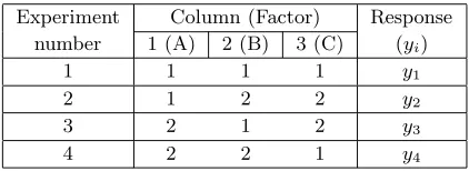
Two level factors are considered as it is recommended by Taguchi for an initial experi-ment. Since only three factors are studied without interaction, an L4 matrix is chosen. The L4, two level matrix is shown in Table 1, where the numbers 1 and 2 stand for the levels of the factors. In data analysis, signal-to-noise (S/N) ratios are used to allow the control of the response as well as to reduce variability about the response. Analysis of variance (ANOVA) is carried out to analyze the relative significance of the individual factors involved.
Table 1: L4 Orthogonal Array
Experiment Column (Factor) Response number 1 (A) 2 (B) 3 (C) (yi)
1 1 1 1 y1
2 1 2 2 y2
3 2 1 2 y3
4 2 2 1 y4
Experiments were performed with the Network Simulator [3]. The simulator was selected because of the range of features that it provides, and partly because it is an open source code that can be modified and extended. All simulations were performed on an Intel Pentium IV processor at 2.00 GHz, 256 MB of RAM running Linux Fedora Core 3. Each simulation scenario was executed for 300 seconds.
The impacts of the factors on the performance of the DSR protocol were examined by looking at drop rate. The desirable results are smaller drop rates, corresponding to higher number of data packets delivered from source to destination in the network. The following factors were considered in the experiment: terrain size, pause time, and node velocity.
xmeter andy meter. The terrain size is adjusted approximately to maintain the required network density [15]. Whereas pause time and node velocity are the most significant factors for the node movement. Both factors face the challenge to the DSR protocol on how to repair broken routes using low overhead [14]. The control factors with the chosen levels are listed in Table 2.
Table 2: Factors and Levels
Symbols Factors Level 1 Level 2 A Terrain (m2
) 25×25 45×45 B Node velocity (m/s) 0.72 1.34 C Pause time (s) 15 50
The justification of the level choices that were made is as follows. The terrain size of 25
×25 m2
and 45×45 m2
could be a place like a meeting room, lecture room, multipurpose room and so forth, where a group of people associated with their wireless devices such as PDAs, cell-phones, and laptops, all termed as hosts, communicate each other.
A pause time is a dormant time taken by a node before moving to another destination, measured in seconds. The pause time here can be when, a shopper acting as a host in a shopping complex, pauses frequently from one location to another to do something, for example window shopping, including surveying and examining the price and quality of items, goods, and clothes, before buying [12]; or when a student, performing as a host, who pauses for a moment at one destination, at his/her friends’ location, to have a talk, discussion, and conversation, before moving to his/her original position or another destination in a classroom.
The speeds of 0.72 m/s and 1.34 m/s are the minimum and the maximum walking speeds of a pedestrian, respectively [11]. In real life, the differences can be explained by the trip purposes of hosts, and the places where they walk [10]. For example, a shopper in a shopping area tends to walk slower compared to a pedestrian in an airport terminal who is usually in a hurry.
The experimental data is shown in Table 3. Each experimental trial corresponds to a simulation scenario. Each simulation scenario was run with three replications (r = 3). The means of the three replications for each trial were then computed. The equation for means is
x=
n X
i=1
xi
n (1)
this type of S/N ratios is
S/N = −10 log [x 2 1+x
2 2+x
2
3+· · ·+x 2 n
n ] (2)
= −10 log (MSD) (3)
= −10 log1 n
n X
i=1
x2i (4)
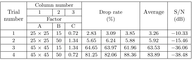
wherenis the number of replications, andxithe value of the metric for theith replication for one trial. In Equation (4), the negative sign is applied to assure a S/N ratio increases for decreasing mean square deviation (MSD with target valuet0= 0). Therefore, a lower mean square deviation which is equivalent to a higher S/N ratio is preferred. The measured results of the drop rate, means, and S/N ratios obtained using Equation (4) for each experimental trial are shown in Table 3.
Table 3: Experimental Layout and Data Collection
Column number
Trial 1 2 3 Drop rate Average S/N
number Factor (%) (dB)
A B C
1 25×25 15 0.72 2.83 3.09 3.85 3.26 −10.33 2 25×25 50 1.34 5.65 6.24 5.88 5.92 −15.46 3 45×45 15 1.34 64.65 63.97 61.96 63.53 −36.06 4 45×45 50 0.72 81.25 82.06 88.36 83.89 −38.48 Note: A: Terrain; B: Pause time; C: Node velocity
3
Results
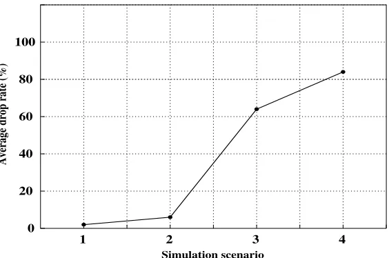
The purpose of this analysis is to visualize the performance of the DSR over the simulation scenario. Upon inspection, the performance of the DSR changes as the factor levels change. Generally, this indicated that, varying the factor settings has influenced the output results (drop rate). As shown in Figure 1, the best condition (trial) that optimizes drop rate is the scenario 1 compared to the others. Obviously, it then increases linearly with the number of simulation scenario. Specifically, in the experiment 1, the terrain is smaller (level 1). This contributes to high connectivity in the networks, and therefore leads to better packets delivery. In addition to small terrain size, the mobility node is also considered so moderate that nodes are not often invalidating the existing routes maintained by the DSR protocol. Regarding this, maximum data packets can be transmitted.
1 2 3 4 0
20 40 60 80 100
Simulation scenario
Average drop rate (%)
Figure 1: The Relative Effects of Factors
Using the experiment matrix, the effects factor was estimated. For clarity, procedure to estimate the effects of factors is illustrated. Let us consider an example of L4 matrix shown in Table 1. Let A1 and A2 be a total of a response value with factor A set at level 1 and level 2, respectively. The average values of a total response with factor A set at level 1 and level 2 are
A1=
y1+y2
2 (5)
A2=y3+y4
2 (6)
Similarly, others can be defined using the following terms,
B1= y1+y3
2 (7)
B2= y2+y4
2 (8)
C1= y1+y4
2 (9)
C2= y2+y3
2 (10)
From Equation (5)-(10), the estimated effects of factor A, B, and C are
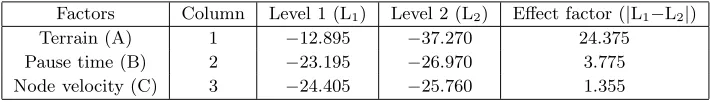
Using the equations above, the effects of factors are estimated, from which the most influential factor, therefore, could be identified. Responses are in terms of S/N ratios, and the results are summarized in Table 4.
As shown in Table 4, the terrain is the most influential factor, affecting the drop rate of the DSR, followed by the pause time; and the node velocity has the least effect on the drop rate of the DSR. Graphically, these relative effects of factors can also be observed in the response graph shown in Figure 2. The factors can be ranked based on the relative comparisons of slopes between points plotted.
As higher S/N is preferred, the level of the factor with the highest S/N values is desired. Thus, according to Table 4 and Figure 2, the best combination factor levels areA1,B1, and C1. Their contributions are shown in Table 5.
If the predicted signal-to-noise ratios based on the selected levels of factors involved is defined asη, the predicted equation can be written as
η=A1+B1+C1−T (14)
where T is grand average of performance (refer Table 6). Since the optimum combination, that isA1,B1, andC1, happens to be the experiment number 1 that is already completed, confirmation test is not needed [9]. Therefore, using the Equation (14), the optimum performance is presented in Table 6, which is similar to that obtained in the experiment 1 (refer Table 3). An estimated result in the original units is 3.26%, in average.
Table 4: S/N Response Table for Factorial Effects
Factors Column Level 1 (L1) Level 2 (L2) Effect factor (|L1−L2|) Terrain (A) 1 −12.895 −37.270 24.375 Pause time (B) 2 −23.195 −26.970 3.775 Node velocity (C) 3 −24.405 −25.760 1.355
Table 5: Factor Contribution
Factors Level description Level Contribution Terrain size 25×25 m2
1 12.1875 Pause time 15 s 1 1.8875 Node velocity 0.72 m/s 1 0.6775
Analysis of variance (ANOVA) was conducted to determine the relative influence of the individual factors and interactios to the total variation of the results. The interactions among the factors were not considered here. The strategy known as pooling was used [9], where factors having lower effects are combined with the error term to provide better estimate of error variance.
Table 6: Optimum Condition
Contribution from all factors (total) 14.7525 Grand average of performance -25.0825 Optimum performance -10.33 Estimated result in the original units (%) 3.26
0
−10
−20
−30
−40
A1 A2 B1 B2 C1 C2
S/N
Figure 2: Response Graph for Factorial Effects
Table 7: ANOVA Table of S/N Ratios
Sources Column f SS V F PSS P(%)
Terrain 1 1 594.161 594.161 324.269∗ 592.329 97.066
Pause time 2 1 14.239 14.239 7.771∗ 12.407 2.033
Node velocity 3 1 1.832 - - -
-Error term 1 1.832 1.832 0.901
Total 3 610.233 100.000
Note: f: Degrees of freedom; SS: Sum of squares; V: Means squares (Variance); F:F-ratio; PSS: Pure sum of squares; P: Percent influence
velocity is considered to be insignificant, the effect of this factor is pooled. The influence of the error term is 0.901%. This small influence of the error term is due to the three sources [8]: experimental error, factors not included in the experiment, and uncontrollable factors. The 0.901% error means that 99.099% (100-0.901) of the influence on the variation of results comes from the two significant factors, which are the terrain size and the pause time.
4
Discussions
The drop rate of the DSR is dependent on the number of packets dropped, which is derived from packet delivery ratio (PDR). The PDR, one of the useful metrics to evaluate any ad hoc routing protocols, is defined as the number of packets delivered to destination (D) divided by the number of packets transmitted by source (T) [5].
Packet delivery ratio (PDR) = D
T (15)
Then, the number of packets dropped is defined as the number of packets transmitted by source minus the number of packets delivered to destination.
Number of packets dropped = T−D (16)
Eventually, the drop rate of the DSR is Drop rate = T−D
D ×100%.
Terrain plays a very important role in determining the performance of the DSR protocol with respect to drop rate. Given larger terrain, nodes could be out of a transmission range of one another, and therefore nodes get partitioned [2]. This could lead to high drop packets. Also, given high mobility, nodes are quickly mobile. This makes a weakened connectivity in the network, as routes are frequently broken. Since pause time corresponds to node mobility, there is, statistically, a reason that an interaction might exist between terrain size and pause time in contributing to the drop rate of the DSR [9].
Also, terrain along with network size and transmission range of nodes determines the node density. Network size and transmission range of nodes can also influence the DSR performance. However, in this work, we decided to fix the size and range as 10 nodes and 10 meter, respectively. IfN is the number of nodes,rthe node’s transmission range, andx and y the width and length of terrain, the network densityT is [13]
T = N r
2 π
xy (17)
High network density contributes to high connectivity in the network. This is because increasing node density leads to better connectivity. Consequently, this directly results in lower drop rate.
Node velocity decides how quickly or slowly the node’s position change, which in turn determines how quickly the network topology changes in the network. Thus, it directly affects how often the existing routes are broken or new routes are established.
The performance of the DSR suffers a bit from high mobility [5]. With high mobility, the possibility of link failures is high, or link failures happen very frequently. It means the DSR protocol may not be able to keep up with the job of establishing routes. To have lower drop rate, high motion should be avoided. In the DSR protocol experiments, besides node velocity, pause time is also a source of node movement. Ifdandv are defined as drop rate and node velocity, respectively, their relationship is
d ∝ v (18)
Drop rate is directly proportional to node velocity. It means that to obtain lower drop rate, node velocity should be low. Ifpis defined as pause time, its relationship to drop rate is
d ∝ 1
p (19)
Here, drop rate is inversely proportional to pause time. It means that, in contrast to node velocity, to get lower drop rate, pause time should be high. Hence, the following relationship is obtained.
d ∝ v
p (20)
Therefore, theoretically, the higher the pause time, and the smaller the node velocity, the smaller the drop rate of the DSR protocol should be.
5
Conclusion
The optimal drop rate for the dynamic source routing protocol was found by using the Taguchi Method. An L4 orthogonal array was used to design the experiments. The results revealed that terrain, pause time, and node velocity can significantly affect the drop rate of the DSR protocol. Among the factors considered, terrain was found to have strong effects, followed by pause time. By taking into consideration of factorial effects, the optimal levels were chosen to be the terrain size of 25×25 m2
, pause time of 15 seconds, and node velocity of 0.72 m/s. Using these factor-levels combination, a minimum of 3.26% drop rate could be obtained. Further studies will investigate the interaction effects between terrain size and pause time.
Acknowledgements
This work was supported by Universiti Teknologi Malaysia (UTM) under Grant Vote No. 79220 and by Ministry of Science, Technology and Innovation (MOSTI), Malaysia, under Grant 01-01-06-SF0234.
References
[2] D.B. Johnson & D.A. Maltz,Dynamic Source Routing in Ad Hoc Wireless Networks,
in: T. Imelinski & H. Korth, eds. Mobile Computing, Kluwer Academic Publisher, Norwell, Mass., 1998, 151–181.
[3] K. Fall & K. Varadhan,ns Notes and Documentation, US Berkeley and Xerox PARC, 1999,URL:http://www.isi.edu/nsnam/ns/
[4] A. Boukerche, Performance Evaluation of Routing Protocols for Ad Hoc Wireless
Net-works,Mobile Networks and Applications, 9(5)(2004), 333–342.
[5] S.R. Das, C.E. Perkins & E.M. Royer, Performance comparison of Two On-Demand
Routing Protocols for Ad Hoc Networks,Proceedings of the IEEE Conference on
Com-puter Communications (INFOCOM), March 2000, Tel Aviv, Israel: IEEE, 3–12. [6] A. Nasipuri, R. Castaneda & S.M. Das, Performance of multipath routing for
on-demand protocols in ad hoc networks, Kluwer Mobile Networks and Application
(MONET) Journal, 6(4)(2001), 339-349.
[7] G.S. Peace,Taguchi Methods: a Hands-on Approach, Addison-Wesley Publishing Com-pany, Reading, Mass., 1993.
[8] Ranjit K. Roy,Design of Experiment Using The Taguchi Approach : 16 step to product
and process improvement, John Wiley & Sons, Inc., Toronto, Canada, 2001.
[9] Ranjit K. Roy,A primer on the Taguchi Method, Van Nostrand Reinhold, New York, N.Y., 1990.
[10] W. H. K. Lam & Chung-yu Cheung, Pedestrian speed/flow relationships for walking
facilities in Hong Kong,Transportation Engineering, 126(4)(2000), 343–349.
[11] S.B. Young,Evaluation of pedestrian walking speeds in airport terminals, Transporta-tion Research Record No. 1674(1999), 20–26.
[12] M. Sarahintu & M.H Lee, Performance Evaluation on Mobile Ad Hoc Networks with
Dynamic Source Routing Protocol,Prosiding Simposium Kebangsaan Sains Matematik
Ke-14, 06–08 Jun 2006, Kuala Lumpur: PERSAMA and UM, 517–523.
[13] R.V. Boppana & A. Mathur, Analysis of the Dynamic Source Routing Protocol for Ad
Hoc Networks, IEEE Workshop on Next Generation Wireless Networks (WoNGeN),
December 18-21, Goa, India, 2005.
[14] D.D. Perkins, H.D. Hughes & C.B. Owen, Factors affecting the performance of ad hoc
networks,Proceedings of the IEEE International Conference on Communications (ICC
2002), 28 April–02 May 2002, New York City, USA: IEEE, vol.4, 2048–2052.
[15] M.W. Totaro & D.D. Perkins, Using statistical design of experiments for analyzing
mobile ad hoc networks, Proceedings of the 8th ACM international symposium on
Modeling, analysis and simulation of wireless and mobile systems, October 10–13, Montreal, Quebec: ACM, 2005, 159–168.
[16] D.A. Maltz, J. Broch, J. Jetcheva & D.B. Johnson,The Effects of On-Demand
Behav-ior in Routing Protocols for Multi-Hop Wireless Ad Hoc Networks, IEEE Journal on
Selected Areas of Communications, 17(8)(1999), 1439–1453.
[17] E.M. Royer & C.K. Toh, A Review of Current Routing Protocols for Ad Hoc Mobile