Multi State analysis of process status using multilevel flow modelling and Bayesian network

(1)

78: 8–3 (2016) 33–41 | www.jurnalteknologi.utm.my | eISSN 2180–3722 |

Jurnal

Teknologi

Full Paper

MULTI–STATE

ANALYSIS

OF

PROCESS

STATUS

USING

MULTILEVEL

FLOW

MODELLING

AND

BAYESIAN

NETWORK

Mohamed A. R. Khalil

a

_{, Arshad Ahmad}

a,b*

_{, Tuan Amran Tuan}

Abdullah

a,b

_{, Ali Al-Shatri}

a

_{, Ali Al-Shanini}

c

a

_{Center of Hydrogen Energy, Institute of Future Energy, Universiti}

Teknologi Malaysia, 81310 UTM Johor Bahru, Malaysia

b

_{Department of Chemical Engineering, Faculty of Chemical & Energy}

Engineering, Universiti Teknologi Malaysia, 81310 UTM Johor Bahru,

Malaysia

c

_{Department of Chemical Engineering, Hadhramout University,}

Mukalla, Yemen

Article history Received 19 May 2015 Received in revised form

24 March 2016 Accepted 1 May 2016

*Corresponding author:

[email protected]

Graphical abstract

Sou5 – heating water source failure

Obj1 – Heating water flow failure

Obj2 – Electrical failure

Tra13 -Pump 2 failure Tube rapture

Sou5

Sou6 Bar0

Sto1 Tra12

Failure in HV 100

Failure in tank VE110

No electrical Tra16

Cord failure Tra13

Mechanical failure Failure in HV

100

Abstract

Multilevel Flow Modeling (MFM) model maps functionality of components in a system through logical interconnections and is effective in predicting success rates of tasks undertaken. However, the output of this model is binary, which is taken at its extrema, i.e., success and failure, while in reality, the operational status of plant components often spans between these end. In this paper, a multi-state model is proposed by adding probabilistic information to the modelling framework. Using a heat exchanger pilot plant as a case study, the MFM model is transformed into its fault tree [1] equivalent to incorporate failure probability information. To facilitate computations, the FT model is transformed into Bayesian Network model, and applied for fault detection and diagnosis problems. The results obtained illustrate the effectiveness and feasibility of the proposed method.

Keywords: Functional modeling, multi–state system, multilevel flow modeling, fault tree

analysis, Bayesian network.

Abstrak

Model Permodelan Pelbagai Aras (MFM) memetakan fungsi-fungsi komponen-komponen dalam sistem secara logical dan ianya berkesan dalam meramal kadar kejayaan tugas yang dilaksanakan. Walau bagaimanapun, keluaran dari model ini adalah binari dengan nilai yang diambil pada titik ekstrema, iaitu sama ada berjaya atau gagal, sedangkan pada keadaan sebenar, status operasi komponen loji sering menjangkau titik-titik di antara kedua ekstrema tersebut. Dalam artikel ini, model pelbagai keadaan dicadangkan dengan menambah maklumat kebarangkalian kepada rangka kerja model. Dengan menggunakan loji perintis penukar haba sebagai kajian kes, model MFM itu ditukar menjadi model yang setara dalam format pokok gagal [1] yang menggabungkan maklumat kebarangkalian kegagalan. Untuk memudahkan pengiraan, model FT itu diubah kepada format model rangkaian Bayesian, dan digunakan untuk permasalahan pengesanan dan diagnosis kerosakan. Keputusan yang diperolehi menggambarkan keberkesanan dan kesesuaian kaedah yang dicadangkan.

Kata kunci: Pemodelan berasaskan berfungsi, sistem pelbagai keadaan, model aliran

pelbagai aras, analisis pokok gagal, rangkaian Bayesian.

(2)

1.0 INTRODUCTION

Multilevel Flow Modelling (MFM) is a functional modelling technique with high level of abstraction, and belongs to a class of artificial intelligence research called qualitative reasoning [2]. The relationship between functions and the objective or main goal of the system in MFM model is determined by cause– effect relationships, based on means–end relations to represent the process in multiple levels of functions [3]. The causal relations between the behaviour and the intention of the system components makes the MFM model suitable for system diagnosis [4], and attracts various applications. Petersen[5] used an MFM model for alarm analysis, risk monitoring systems and fault analysis, while Larsson[6] used MFM model to describe the target of the process for measurement validation, alarm analysis and fault diagnosis.

Despite these encouraging reports, the

conventional MFM model is not attractive for general use in chemical processes as it only provides binary outputs at its extrema. For applications in chemical processes, models that provide multiple states are more useful compared to those that describe the system and its components as (0, 1) and ignores their intermediate states [7, 8]. This has encouraged the development of modelling frameworks such as multi–state event tree and multi–state fault tree [9-11]. The idea of using multi– state system in engineering was popularised by [12] by expressing the expected outcomes in terms of failure probabilities or frequencies. In this paper, this idea is adopted to extend the functionality of the MFM model for the purpose of fault detection and diagnosis. By converting the fault tree developed from the MFM model into Bayesian network, the desired analysis of multi–state system can be carried out using conditional probability distribution to represent the relationship between components states and system target.

2.0 THE CAUSALITY SYSTEM IN MFM

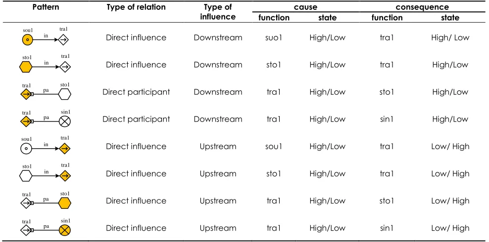
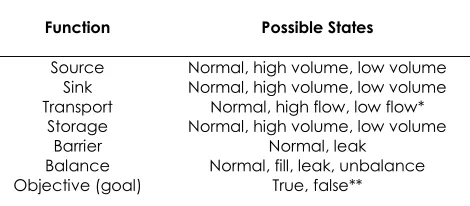
In this paper, causal dependency graphic (CDG) is used to represent the qualitative cause–consequences analysis between components in the MFM model. The states of the MFM flow functions are shown in table 1. Each function in the MFM model may only take some of these states. Besides, to guarantee success in achieving the main goal, each function must be in a normal state [13]. According to these states the CDG of system is constructed.

Table 1 The states of flow functions in MFM

Function Possible States

Source Normal, high volume, low volume Sink Normal, high volume, low volume Transport Normal, high flow, low flow*

Storage Normal, high volume, low volume

Barrier Normal, leak

Balance Normal, fill, leak, unbalance Objective (goal) True, false**

*No flow state is included as low flow state. **False state of an objective function in divided to two states, false results from the high state of functions (fault -1) while the consequences of the low state of functions is (Fault - 2).

3.0 BAYESIAN NETWORK (BN)

BN is a probabilistic graphical model that is based on directed acyclic graphs (DAG) with probability annotated. A node in a BN represents a random variable, and is linked with other variables with defined probabilistic dependencies. Using BN, qualitative and quantitative representation of the relations between variables can be established using prior and conditional probabilities of variables. Updates of these probabilities can be generated and used to represent different system probabilities. The “OR” gate in fault tree model is mapped to BN, and is equivalent to a series system, while the “AND” gate is equal to parallel system. By using BN, compactness of the model can be established by factoring the joint distribution into a local, conditional distribution for each variable given its parents. If xi denotes a value of the variable Xi and pai denotes some set of values for the parent of Xi, then P(xi | pai) denotes this conditional distribution.

4.0 CASE STUDY:

As a case study, a heat exchanger pilot plant system at Universiti Teknologi Malaysia normally used for studying heat exchange mechanisms and temperature control is examined. As illustrated in Figure 1, the plant consists of a heating medium tank (VE110), product tank (VE150), two pumps (P112, P152), heat exchanger (HX120), cooler (CL140), two heaters (HE110, HE111) and valves. Water is supplied to this plant from outside sources via hand valve HV100 and HV101 to the heating medium tank VE110 and product tank VE150

respectively. Then the water in VE110 is heated to 60 o_C

(3)

4.1 Multilevel Flow Modelling (MFM) for The Heat Exchanger Pilot Plant

The heat exchanger pilot plant illustrated in Figure 1 is converted into the MFM model and is shown in Figure 2. Note that the control systems of the plant plays important role for plant operation and safety, but is not included in this study. This process has one goal (main goal) (Go0), which is to maintain water temperature in tank VE150, and five objectives (sub - goals) for more details (Khalil et al., 2016). In this plant, heat exchanger

is the core of the system. It has two purposes, the main function is to transfer energy from the hot water to the cold water, and a secondary purpose to prevent mixing between hot and cold water via tube wall that represents in the model by barrier (Bar0). The heat exchange mechanism is represented by the balance function in the MFM model, Bal3 and Bal6 for cooling and heating water respectively for mass flow, and by Bal10 and Bal12 for energy flow structure (EFS0).

Figure 1The heat exchanger pilot plant [14]

Figure 2 The MFM of the heat exchanger pilot plant [14] HV136

HV154

HV100

FY121

P112 HV124

HX120

VE150

P152 HV111

HV134 CL140

HV141

HV101

T

Temp. Sensor

HV150 HV110

VE110 HE110

Tra4

Sou4

Sou6 Sou3

Sou2

Sou1 Sou0

Sou5

Sin0

Sin1

Sin2

Sin3

Sin4

Sin6

Sin5

Tra1 Tra2

Tra0 Bal0

Tra6

Tra3

Tra5

Tra10

Tra7 Tra8 Tra9

Tra11 Sto0

Sto1

Tra16

Tra12 Tra13 Tra14 Tra15

Bal1

Bal2

Obj0

Bal3 Bal4

Bal5 Bal6 MFS0

Bar0

Tr

a1

6

Tr

a1

1

Tr

a6

Tr

a1

4

Tr

a8

Go0

Obj1

Obj2 Obj3

Obj4

EFS3

EFS2

(Keep the pump2 running) MFS1

EFS1

EFS0

in0 pa0 in1 pa1

in3

pa2 in2

pa3

in 5

pa

5

in4 pa4

in6 pa6

in7 pa7 in8 pa8 in9 pa9

in12 pa12 in13 pa13 in14 pa14 in15 pa15 in10 pa10

in11 pa11

in16 pa16

in17 pa17

(Keep the pump1 running)

(Keeping the flow of cooling water)

(Keeping the flow of heating water) (Maintaining the temp.

in the product tank)

(Heating water in the VE110)

Mass flow of cooling water

Energy flow in pump

Mass flow of heating water Energy flow in heater

Energy flow of heating water Enery flow of cooling

water

m

a0

en a0

pp

0

m

a4

ena4

m

a1

ena1

m

a2

ena2

m

a3

ena3

Tr

(4)

4.2 Fault Tree of MFM

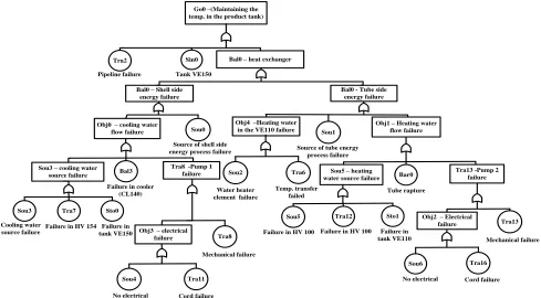
Figure 3 shows the fault tree model that is mapped from MFM model to incorporate probabilistic information into the modelling framework. The FT model represents the relationship between events of

the heat exchanger pilot plant, with the top event TE assumed to occur when a fault is occurring in only one component at any time. Note that in this analysis, the prior probability distributions of basic components are considered independent.

Go0 –(Maintaining the temp. in the product tank)

Sou5 – heating water source failure Bal0 – heat exchanger

Bal0 - Tube side energy failure

Obj1 – Heating water flow failure Bal0 – Shell side

energy failure

Sou3 – cooling water source failure

Obj0 – cooling water flow failure

Tra8 -Pump 1 failure

Obj2 – Electrical failure

Tra13 -Pump 2 failure

Obj3 – electrical failure

Sin0 Tra2

Obj4 –Heating water in the VE110 failure Pipeline failure

Source of shell side energy process failure

Failure in cooler (CL140)

Tank VE150

Sou0

Tra6 Bal3

Sto0

Tra8

Sou1

Sou3 Tra7

Cooling water source failure

Failure in tank VE150

Tube rapture

Failure in HV 154

Source of tube energy process failure

Cord failure No electrical

Mechanical failure

Sou4 Tra11

Sou5

Sou6

Sou2 Bar0

Water heater element failure

Temp. transfer failed

Sto1 Tra12

Failure in HV 100 Failure in

tank VE110

No electrical

Tra16

Cord failure Tra13

Mechanical failure Failure in HV 100

Figure 3 The FT of the MFM of the heat exchanger pilot plant [14]

Note that in Figure 3, all gates are “Or”, reflecting that the components can be represented by a series system in the MFM model. TE represents the failure to maintain water temperature in tank VE150 at the desired set point. Since this is the main function of the plant, for the MFM model, it is considered as the main goal. The failure to satisfy this main goal may results from the failure in one or more intermediate gates, i.e., Bal0 (heat exchanger fails to functioning) which results from the failure in the tube or shell sides, Obj0 (failure to cool water), Obj1 (heat exchanger fails to heat a water), Obj2 (electrical failure to provide electricity to the pump 2), Obj3 (electrical failure to provide electricity to the pump 1), Obj4 (heater in tank V110 fails to heat a water), Tra8 (pump 1 fails to transfer the cool water to the heat exchanger), Tra13 (pump 2 fails to transfer the water), Sou3 (failure to provide the system for the cold water), Sou5 (failure to provide the system for the hot water). All these will lead to the TE being false. The fault tree model of the system included only significant changes of plant states that are dependent on implicit assumptions about plant functions and operating conditions.

(5)

Sou5 tra12 highvol

Normvol

lowvol

highflow Normflow

lowflow

sto1 tra13 Bal5 tra13 Bal6

highvol Normvol

lowvol

lowflow

lowflow Fill

Normvol

Leak

Fill Normvol

Leak

tra15 highflow Normflow

lowflow

Sin5 highvol Normvol

lowvol

Figure 4The Causal Dependency Graph between functions of the MFM in Figure2.

According to Table 1, the components are set in three states 0, 1, 2, where 0 is normal operation state, 1 is a state of fault state 1(high or fill), 2 is fault state 2 (low or leak). Unbalance state is included in the leak

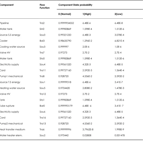
state in this study. The prior probability distributions of root nodes of the system shown in Table 3 are obtained by statistics and analysis of failure data of the elements of the system.

Table 2 Direct influences relationships between flow functions in MFM model in Figure 2

Pattern Type of relation Type of

influence function cause state function consequence state

sou1 tra1

in _{Direct influence} _Downstream _suo1 _High/Low _tra1 _{High/ Low}

sto1 tra1

in _{Direct influence} _Downstream _sto1 _High/Low _tra1 _High/Low

tra1

pa sto1 _{Direct participant} _Downstream _tra1 _High/Low _sto1 _High/Low

tra1

pa sin1 _{Direct participant} _Downstream _tra1 _High/Low _sin1 _High/Low

sou1 tra1

in _{Direct influence} _Upstream _sou1 _High/Low _tra1 _{Low/ High}

sto1 tra1

in _{Direct influence} _Upstream _sto1 _High/Low _tra1 _{Low/ High}

tra1

pa sto1 _{Direct influence} _Upstream _tra1 _High/Low _sto1 _{Low/ High}

tra1

pa sin1 _{Direct influence} _Upstream _tra1 _High/Low _sin1 _{Low/ High}

Prediction

(6)

Table 3 Prior probability distribution of root nodes of the system in Figure 3

Component Flow

Function Component State probability

0 (Normal) 1(High) 2(Low)

Pipeline Tra2 0.9999934552 6.48E-6 6.48E-8

Water tank Sin0 0.99983869 1.598E-4 1.512E-6

Source S.S energy Sou0 0.99321220 6.48E-3 3.078E-4

Cooler Bal3 0.98635790 1.296E-2 6.821E-4

Cooling water source Sou3 0.999997 2.0E-6 1.0E-6

Valve HV Tra7 0.97273 2.7E-2 2.7E-4

Water tank Sto0 0.99983869 1.598E-4 1.512E-6

Electricity supply Sou4 0.99561520 4.32E-3 6.48E-5

Cord Tra11 0.99727160 2.592E-3 1.364E-4

Pump1 mechanical Tra8 0.928720 4.536E-2 2.592E-2

Source T.S energy Sou1 0.99999318 6.48E-6 3.41E-7

Heating water source Sou5 0.9704420 2.808E-2 1.478E-3

Valve HV Tra12 0.97273 2.7E-2 2.7E-4

Tank Sto1 0.99983869 1.598E-4 1.512E-6

Tube rupture Bar0 0.999993179 6.48E- 6 3.41E- 7

Electricity supply Sou6 0.99561520 4.32E-3 6.48E-5

Cord Tra16 0.99727160 2.592E-3 1.364E-4

Pump2 mechanical Tra13 0.928720 4.536E-2 2.592E-2

Heat transfer medium Tra6 0.99999996 3.7962E-8 1.998E-9

Water heater elem. Sou2 0.970442 0.02808 0.001478

5.0 RESULT AND DISCUSSION

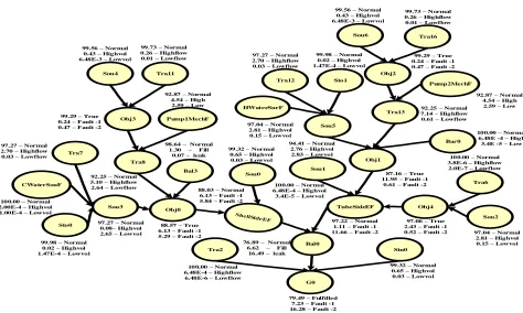
Based on the BN model of the heat exchanger, using the prior probability of components and the CPT of the top event (G0), and by applying accurate reasoning Bucket elimination algorithm [15] to calculate the probability, the probabilities are determined, giving value for the node G0, P(G0 = FAULT-1) = 0.0723, P(G0 = FAULT-2) = 0.1628, as shown in Figure 5. Note that in cases of no evidence, the probability of node G0 and intermediate nodes cannot be determined.

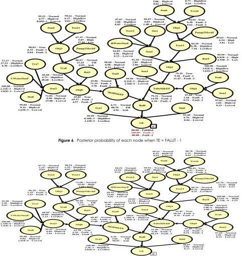
Similarly, the posterior probability of each node can be deduced when the system is in completely

fault-1 state (G0 (FAULT-1) = 1) or in case of completely fault–2 state (G0 (FALUT–2 = 1), as is shown in Figure 6, Figure 7.

In the case of given evidence that G0 is completely fault state (G0 = FALUT-1 or G0 = FALUT-2), all conditional probabilities for component nodes can be calculated.

(7)

Table 4 The failure probability of each component when system top node (TE) fault

Component

node Tra2 Fault -1 Fault -2 Sin0 Fault -1 Fault -2 Sou0 Fault -1 Fault -2

G0 (Fault -1) 8.18E-5 2.15E-7 6.76E-2 4.0E-4 9.8E-3 3.3E-3

G0 (Fault -2) 3.3E-6 3.01E-7 9.6E-3 1.7E-3 3.49E-2 4.0E-4

Component

node Bal3 Fault -1 Fault -2 Sto0 Fault -1 Fault -2 CWaterSouF Fault -1 Fault -2

G0 (Fault -1) 0.1324 9.0E-4 1.6E-3 1.63E-5 2.21E-5 1.02E-5

G0 (Fault -2) 1.93E-2 3.7E-3 2.0E-4 1.61E-6 2.19E-6 1.47E-6

Component

node Tra7 Fault -1 Fault -2 Pump1MechF Fault -1 Fault -2 Sou4 Fault -1 Fault -2

G0 (Fault -1) 0.2753 3.0E-3 5.07E-2 0.2755 7.7E-3 8.85E-5

G0 (Fault -2) 3.99E-2 3.0E-4 0.2499 3.33E-2 2.24E-2 3.0E-4

Component

node Tra11 Fault -1 Fault -2 Sou1 Fault -1 Fault -2 Bar0 Fault -1 Fault -2

G0 (Fault -1) 3.7E-3 2.0E-4 8.31E-5 2.56E-7 8.01E-5 6.93E-7

G0 (Fault -2) 1.39E-2 7.0E-4 2.38E-6 1.95E-6 3.51E-6 1.75E-6

Component

node HwaterSouF Fault -1 Fault -2 Tra12 Fault -1 Fault -2 Sto1 Fault -1 Fault -2

G0 (Fault -1) 4.96E-2 1.5E-3 2.88E-2 5.0E-4 3.0E-4 1.6E-6

G0 (Fault -2) 0.1466 8.2E-3 0.1493 8.2E-3 8.0E-4 8.12E-6

Component

node Sou6 Fault -1 Fault -2 Tra16 Fault -1 Fault -2 Pump2MechF Fault -1 Fault -2

G0 (Fault -1) 5.06E-2 1.0E-4 7.7E-3 1.6E-3 6.54E-2 3.81E-2

G0 (Fault -2) 3.4E-3 3.0E-4 1.21E-2 1.0E-4 0.2433 0.1387

Tra16 Sou6

Obj2

Pump2MechF

Tra13

Obj1

Bar0 HWaterSurF

Sto1 Tra12

Sou5

TubeSideEF

Tra6

Sou2 Sou1

Obj4 CWaterSouF

Sto0 Tra7

Sou3

Bal0

Sin0

G0 Tra2

Sou0 Bal3

Obj0 Pump1MechF Obj3

Tra8

Sou4 Tra11

79.49 – Fulfilled 7.23 – Fault -1 16.28 – Fault -2 100.00 – Normal

6.48E-4 – Highflow 6.48E-6 – Lowflow 97.27 – Normal

2.70 – Highflow 0.03 – Lowflow

99.32 – Normal 0.65 – Highvol 0.03 – Lowvol 76.89 – Normal

6.62 – Fill 16.49 – leak 97.27 – Normal

0.08– Highvol

2.65 – Lowvol 97.04 – Normal

2.81 – Highvol 0.15 – Lowvol 100.00 – Normal 3.8E-6 – Highflow 2.0E-7 – Lowflow 87.16 – True

11.95 – Fault -1 0.61 – Fault -2

97.06 – True 2.43 – Fault -1 0.52 – Fault -2 97.22 – Normal

1.11 – Fault -1 11.66 – Fault -2

100.00 – Normal 6.48E -4 – High 3.4E -5 – Low 92.25 – Normal

92.87 – Normal 4.54 – High 2.59 – Low 99.29 – True

0.24 – Fault -1 0.47 – Fault -2 99.73 – Normal 0.26 – Highflow 0.01 – Lowflow 99.56 – Normal

0.43 – Highvol 6.48E-3 – Lowvol

100.00 – Normal 6.48E-4 – Highvol

3.4E-5 – Lowvol

99.98 – Normal 0.02 – Highvol 1.47E-4 – Lowvol

2.81 – Highvol 0.15 – Lowvol 97.27 – Normal 2.70 – Highflow 0.03 – Lowflow

99.98 – Normal 0.02 – Highvol 1.47E-4 – Lowvol 99.56 – Normal

0.43 – Highvol 6.48E-3 – Lowvol

99.73 – Normal 0.26 – Highflow 0.01 – Lowflow

0.24 – Fault -1 0.47 – Fault -2

1.30 – Fill 0.07 – leak

88.03 – Normal 6.13 – Fault -1 5.84 – Fault -2

100.00 – Normal 2.00E-4 – Highvol 1.00E-4 – Lowvol

(8)

Tra16 Sou6 Obj2 Pump2MechF Tra13 Obj1 Bar0 HWaterSurF Sto1 Tra12 Sou5 TubeSideEF Tra6 Sou2 Sou1 Obj4 CWaterSouF Sto0 Tra7 Sou3 Bal0 Sin0 G0 ShellSid_eEF Tra2 Sou0 Bal3 Obj0 Pump1MechF Obj3 Tra8 Sou4 Tra11

00.00 – Fulfilled

100.00 – Fault -1

00.00 – Fault -2 99.99 – Normal

8.18E-3 – Highflow 2.15E-5 – Lowflow 72.17 – Normal

88.70 – Fill 4.56 – leak 72.02 – Normal

0.90– Highvol

27.08 – Lowvol 97.03 – Normal

9.28 – Fault -1 11.43 – Fault -2

14.58 – Fault -1 6.10 – Fault -2

89.65 – Normal 6.54 – High 3.81 – Low 94.01– True

5.06 – Highvol 0.01 – Lowvol

99.99 – Normal 8.31E-3 – Highvol

2.56E-5 – Lowvol

4.96 – Highvol 0.15 – Lowvol 97.07 – Normal 2.88 – Highflow 0.05 – Lowflow

0.77 – Highvol 8.85E-3 – Lowvol

0.33 – Fault -1 0.84 – Fault -2

13.24 – Fill 0.09 – leak

25.85 – True 69.57 – Fault -1

4.57 – Fault -2 66.66 – Normal

100.00 – Normal 2.21E-3 – Highvol 1.02E-3 – Lowvol

e

Figure 6 Posterior probability of each node when TE = FALUT - 1

Tra16 Sou6 Obj2 Pump2MechF Tra13 Obj1 Bar0 HWaterSurF Sto1 Tra12 Sou5 TubeSideEF Tra6 Sou2 Sou1 Obj4 CWaterSouF Sto0 Tra7 Sou3 Bal0 Sin0 G0 ShellSideEF Tra2 Sou0 Bal3 Obj0 Pump1MechF Obj3 Tra8 Sou4 Tra11

00.00 – Fulfilled 00.00 – Fault -1

100.00 – Fault -2

100.00 – Normal 3.3E-3 – Highflow 3.01E-5 – Lowflow 95.98 – Normal

1.06 – Fill 98.87 – leak 95.97 – Normal

0.09– Highvol

3.94 – Lowvol 97.04 – Normal

68.24 – Fault -1 0.31 – Fault -2

0.30 – Fault -1 68.24 – Fault -2

61.79 – Normal 24.33 – High 13.87 – Low 98.42– True

0.34 – Highvol 0.03 – Lowvol

100.0 – Normal 2.38E-4 – Highvol

1.95E-4 – Lowvol

14.66 – Highvol 0.82 – Lowvol

84.92 – Normal 14.93 – Highflow

0.14 – Lowflow

2.24 – Highvol 0.03 – Lowvol

71.68 – Normal 24.99 – High

3.33 – Low 96.28 – True

1.29 – Fault -1 2.43 – Fault -2

1.29 – Fill 2.43 – leak

28.68 – Highflow 3.23 – Lowflow 100.00 – Normal

2.19E-4 – Highvol 1.47E-4 – Lowvol

e

Figure 7 Posterior probability of each node when TE = FALUT - 2

6.0 CONCLUSION

A multi-state functional model based on MFM that has been transformed into an equivalent BN model has been used for fault detection and diagnosis in a heat exchanger pilot plant. Qualitative analyses have been represented by causal dependency graph (CDG) and failure probabilities of the root nodes as a quantitative analysis has been applied in a heat exchanger pilot plant. The results show the strength of this approach and can be considered as a useful

strategy for dealing with complex chemical processes.

Acknowledgement

(9)

References

[1] Ericson, C. A. 2005, Hazard Analysis Techniques for System

Safety: John Wiley & Sons, Inc., 2005: 183.

[2] Lind, M. 2011a. Nuclear Safety and Simulation. 2: 22. [3] Lind, M. 2011b. Advances in Safety, Reliability and Risk

Management: ESREL 2011. 383.

[4] Gofuku, A., S. Koide, N. Shimada. 2006. SICE-ICASE.

International Joint Conference: IEEE, 2006: 497.

[5] Petersen, J. 2000. Proceedings of the cognitive systems

engineering in process control (CSEPC 2000). 36.

[6] Larsson, J.E. 2002. Knowledge-Based Systems, 2002: 103. [7] Mi, J., Y. Li, H.-Z. Huang, Y. Liu, X. Zhang. 2012. Quality,

Reliability, Risk, Maintenance, and Safety Engineering (ICQR2MSE). International Conference on: IEEE, 2012: 1117.

[8] Caldarola, L. 1980. Nuclear Engineering and Design. 58: 127.

[9] Yi, R., K. Leixing. 2011. Reliability, Maintainability and Safety (ICRMS), 9th International Conference on, 2011: 920. [10] Kai, Y. 1990. Reliability Engineering & System Safety. 28: 1. [11] Bossche, A. 1984. Microelectronics Reliability. 24: 707. [12] Barlow, R. E., A. S. Wu. 1978. Mathematics of Operations

Research. 3: 275.

[13] Dahlstrand, F. 1999. Research and Development in Expert

Systems XV. 173.

[14] Khalil, M. A. A., Arshad. Abdullah, Tuan Amran T. Al-shanini, Ali. 2016. Chemical Product and Process Modeling. [15] Dechter, R. 1998, Learning In Graphical Models: Springer,