Jurnal Teknologi, 45(C) Dis 2006: 67–84 © Universiti Teknologi Malaysia
STATISTICAL APPROACH ON GRADING THE STUDENT ACHIEVEMENT VIA NORMAL MIXTURE MODELING
ZAIRUL NOR DEANA MD DESA1, ISMAIL MOHAMAD2, ZARINA MOHD
KHALID3 & HANAFIAH MD ZIN4
1
Department of Foundation Education, Faculty of Education, Universiti Teknologi Malaysia, 81310 UTM Skudai, Johor, Malaysia
2,3&4
Department of Mathematics, Faculty of Science, Universiti Teknologi Malaysia, 81310 UTM Skudai, Johor, Malaysia
Abstract. The purpose of this study is to compare results obtained from three methods of assigning letter grades to students’ achievement. The conventional and the most popular method to assign grades is the Straight Scale method (SS). Statistical approaches which used the Standard Deviation (GC) and conditional Bayesian methods are considered to assign the grades. In the conditional Bayesian model, we assume the data to follow the Normal Mixture distribution where the grades are distinctively separated by the parameters: means and proportions of the Normal Mixture distribution. The problem lies in estimating the posterior density of the parameters which is analytically intractable. A solution to this problem is using the Markov Chain Monte Carlo approach namely Gibbs sampler algorithm. The Straight Scale, Standard Deviation and Conditional Bayesian methods are applied to the examination raw scores of two sets of students. The performances of these methods are measured using the Neutral Class Loss, Lenient Class Loss and Coefficient of Determination. The results showed that Conditional Bayesian outperformed the Conventional Methods of assigning grades.
Keywords: Grading methods, educational measurement, Straight Scale, Standard Deviation method, Normal Mixture, Markov Chain Monte Carlo, Gibbs sampling
Abstrak. Kajian dijalankan untuk membanding keputusan yang didapati daripada tiga kaedah penggredan terhadap pencapaian pelajar. Kaedah konvensional yang popular adalah kaedah Skala Tegak. Pendekatan statistik yang menggunakan kaedah Sisihan Piawai dan kaedah Bayesian bersyarat dipertimbangkan untuk memberi gred. Dalam model Bayesian, dianggapkan bahawa data adalah mengikut taburan Normal Tergabung di mana setiap gred adalah dipisahkan secara berasingan oleh parameter; min dan kadar bandingan dari taburan Normal Tergabung. Masalah yang timbul adalah sukar untuk menganggarkan ketumpatan posterior bagi parameter tersebut secara analitik. Satu penyelesaiannya adalah dengan menggunakan pendekatan Markov Chain Monte Carlo iaitu melalui algoritma pensampelan Gibbs. Kaedah Skala Tegak, kaedah Sisihan Piawai dan kaedah
Bayesian bersyarat diaplikasikan untuk markah mentah peperiksaan bagi dua kumpulan pelajar. Pencapaian ketiga-tiga kaedah dibandingkan melalui nilai Kehilangan Kelas Neutral, Kehilangan Kelas Tidak Tegas dan Pekali Penentuan. Didapati keputusan dari kaedah Bayesian bersyarat menunjukkan penggredan yang lebih baik berbanding kaedah Skala Tegak dan kaedah Sisihan Piawai.
1.0 INTRODUCTION
Assigning grades is a compulsory part in education. By the time, the instructor is responsible to assign grades meaningfully where they can apply the Norm Referenced or Criteria Referenced in assigning the letter grades. For students, grade may vary due to differences in the willingness to trade off leisure for study or in the ability to learn a subject, which generates a direct relation between student grades and student learning. For that reason, understanding the relationship between grading practices and student evaluation is important in higher education. Grade is defined as the instructor’s assessment and evaluation of student’s achievement relative to some criteria. It also describes the student’s level of educational progress and universally means of documenting student achievement.
In assigning marks to a student by administering the mid term test, project or examination, by transforming their performance into a form of numbers of letter grades, the instructors should know the procedure to measure the students performance. There are many schemes to assign grades either followed the norm or criterion-referenced which all seem to have their advantages and disadvantages.
There is a classification scheme on various sorts of score that may be used to report the student’s achievement. If the instructor decides to assign the grades to the norm group of a class then the instructor must define the mean and standard deviation of the class’s scores precisely. Then the instructor needs to transform the score into linear standard scores such as z-scores and T-scores. Note that the variance from each graded component must have the same variance as the composite scores.
Generally, the educators often wish to give weight to some components more heavily than others. For example, quizzes scores might be valued at the same weight as a project. A number of studies indicate that the key for proper weighting is by testing the variability of the scores. A practical solution to combining several weighting components is first to transform raw scores to standardized scores; z-score or McCall T-scores [1 – 4 ]. This grading method, called “grading on the curve” or “grading on the normal curve” became popular during the 1920’s and 1930’s. Grading on the curve is the simplest method to determine what percentage of the class would get A’s (say the top 10% get an A), what percentage for B’s, and so on [5]. Grading on curve is a straightforward grading method, but it has serious drawbacks. The fixed percentages are nearly determined arbitrarily. In addition, the used of normal curve to model achievement in a single classroom is generally inappropriate, except in large required course at college or university level [6]. Grading on curve is efficient from an educator point of view.
that describes the dispersion, variability or spread of scores around average score. Unlike grading on curve, this method requires no fixed percentage in advanced.
In moving from scores to grades, educators can grade on an absolute grading scale (say 90 to 100 is an A). Given that the students only care about their relative rank, which kind of grading is better? Works by Pradeep and John [7] have shown that if the students are disparate identical, then absolute grading is always better than grading on a curve. This shows that when all the students are disparate identical, it is always better to grade according to an absolute scale.
2.0 MATERIAL AND METHODS
The students’ raw scores from the selected courses are the subject of interest and are given by the senior instructor. The documents of the students’ raw score are used as evidence. Two sets of student of a small and a large class size are considered. We have assume that every student in a particular class differs to some degree in their psychology and sociology traits.
(i) Measurement
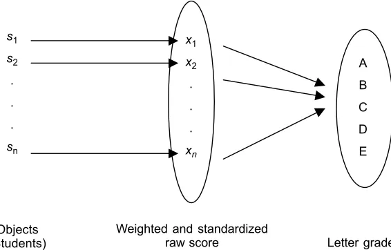
From the definitions, a measurement is the process of assigning numerals to object, events, or people using rule. Ideally the rule assigns the numerals to present the amounts of specific attribute possessed by the objects, events, or people being measured [3]. In this research, we precisely define measurement as the grading process of assigning raw score and a letter grade to a student. Thus the illustration in Figure 1 shows that the grades in mathematical terms of measurement is a functional
Weighted and standardized raw score
Figure 1 A functional mapping of letter grades
Objects
(Students) Letter grades
s1 s2 . . . sn
x1 x2 . . . xn
mapping from the set of objects (i.e. students) {si ; i is the ID of each student}to the set of real numbers of the standardized raw score {xi; xi ∈¡} and i, n ∈ ‚ starting from 1 until n finite number of students.
First, the standardized raw scores are ranked in descending order that is
x1>x2> ... xn. The point of this study is to define the probability set function of the raw scores that belong to the letter grades accordingly. A probability set function of raw score tells us how the probability is distributed over various subsets of raw score in a sample space G.
In addition, a measure of grades is a set function, which is an assignment of a number µ(g) to the set g in a certain class. If G is a set whose points correspond to the possible outcomes of a random experiment, certain subsets of G will be called “events” and assigned a probability. Intuitively, g is an event if the question “Does w
(say 85) belong to g (say A)?” has a finite yes or no answer. After the experiment is performed and the outcome should correspond to the point 85 ∈ G [8].
We denote G as a sample space of grades g1 = E, g2 = D, g3 = D +,...,
g11 = A; {gL∈ G} and the subscript L = 1, 2, …, 11 denotes the eleven components of letter grades. We defined the eleven letter grade components as the set of {A, A–, B+, B, B–, C+,C, C-, D+, D, E} corresponding to the set of grade point averages {4.0, 3.7, 3.3, 3.0, 2.7, 2.3, 2.0, 1.7, 1.3, 1.0, 0.0 }.
2.1 Methodology
In this study, the methodology used is known as Bayesian Grading (we denote as GB). In general, GB is applying Bayesian inference through Bayesian network in classifying a class of students into several different subgroups where each of them corresponds to possible letter grades.
The method has been developed according to Distribution-Gap grading method in finding the grades cutoffs. This is formed by ranking the composites score of students from high to low that is in the form of a frequency distribution. The frequency distribution is cautiously observed for gaps where for several short intervals in the consecutive score range there are no students obtained. A horizontal line is drawn at the top of the first gap which gives an As’ cutoff and a second gap is required. This process continues until all possible letter grade ranges (A-E) have been recognized.
(i) Bayesian methods for mixtures
The earlier understanding and experience of the instructor’s belief in assigning the letter grade is called the “prior belief” and the new belief that results from updating the prior belief is called the “posterior belief”. Prior probabilities are the degree of belief the instructor has prior to observing any raw scores. The posterior probabilities are the probabilities that results from Bayes’ theorem. The posterior probabilities of mutually exclusive and exhaustive events must sum to one for them to be reliable probabilities [10].
In this study, we consider a finite mixture model in which raw scores data X = {x1, x2,..., x3} are assumed to be independent and identically distributed from a mixture distribution of g components. Equation (1) is called the mixture density which the mixture proportion constrained to be non-negative and sum to unity. In other words, Equation (1) is the probability that a particular raw score belongs to a component of the mixture proportional to the ordinate of that component at the raw score. Simplifying, we say that p(x1) is the probability density function of particular raw score. Therefore for all raw scores we have a mixtures density of normal distribution. Our interests are to find the probability that a particular raw score belongs to a component of the mixture normal. The raw scores are independently and identically with the mixture normal distribution. The mixture density has mixed probabilities of πg as follows:
( )
(
2)
1
,
G
i g g g
g
p x π φ µ σ =
=
∑
for i = 1,2,...,n (1)where xi is the raw score of student, g is the indicator of G = 11 components of the mixture, πg is the component probability of component g and it can be written as π = {π1, π2,..., πg}that cannot be negative and
∑
π =1.φ( )
⋅ denotes the parametric component density function where µg and σ2gare mean and variance of componentg and written in the form of vectors µ = {µ1,µ2,...,µg}and σ2 =
{
σ σ12, 22, ,σg2}
.We denote θ1 =
{
π µ σ1, 1, 12}
,θ2 ={
π µ σ2, 2, 22}
, ,θg ={
π µ σg, g, g2}
and therefore, we simplify the sets of θ as equal to Θ ={
θ θ1, ,2 ,θg}
.(ii) Prior and posterior distributions
In this study, we have chosen the conjugate prior implementation to the posterior distribution. The distribution f
( )
xθ =N(
x µ σ, 2)
is a normal density with parameter µ and σ2 and the mean is normally distributed with parameter ν and δ2 (i.e. µ∼N (ν, δ2)), the variance is inverse Gamma distributed with parameter α and β (i.e. σ2 ∼ IG (α, β) and the component probability is Dirichlet distributed with parameter η (i.e. π ∼ Di(η)). We may refer to such distribution as a noninformative prior for Θ. The posterior distribution is proportional to the product of likelihood and prior distribution. That is:f{π, µ, σ2|G, xxxxx}α L {xxx| G, xx π, µ, σ2} h {π, µ, σ2} (2)
The conditional distribution for posterior µg is µg N V M V
(
g g, g1)
−
∼ where
1
2 2 2 2
1
, i
i
g g x g
g g
g g g g
x n
V M ν
δ σ δ σ − ∈ = + = +
∑
that is νg and δ2g are the mean and variance
for each of component g. The conditional distribution for posterior σ2g is
(
)
2 12 / 2, 1 1 2 .
i
g g g g i g
x g
IG n x
σ α β µ − − ∈ + + −
∑
∼(iii) Markov Chain Monte Carlo (MCMC) and Gibbs sampler
In letter grades assigning problem, we are interested to find the optimal mean values for each well defined grades component. Herein, we would like to find the unknown parameter θ of the posterior density. Suppose θ∼ p(θ) and if we seek
(
)
(
)
(
)
(
)
1 , , , , , , , , 1 , , Gt t t g
E p p d
p N θ µ σ π µ σ π µ σ π µ σ π µ σ π = = ≈
∫
∑
x x (3)One problem with applying the Monte Carlo integration is in obtaining samples from one complex probability distribution p(xxxxx). This problem is overcome by Markov Chain Monte Carlo methods (MCMC). The objectives of MCMC are to generate a sample from a joint probability distribution of posterior and to estimate expectation of parameters. The most general MCMC approach is called the Metropolis-Hasting algorithm (M-H algorithm) [12]. A second technique for constructing MCMC is by Gibbs sampling algorithm.
Gibbs sampling is defined in terms of subvectors of θ. Suppose the parameter θ from raw scores have been divided into g components or subvectors, Θ = {θ1,θ2,...,θg}
of the iteration. The Gibbs sampler is cycles through the subvectors of Θ, in which the subset conditional on the value of all the others. There are g steps in iteration t. At each iteration t, an ordering of the g subvectors of Θ is chosen and, in turn, each
t j
θ is sample from the conditional distribution of the mixture normal distribution given all the other components of Θ: p
(
θg XXXX,Θt−−j1)
where Θt−−j1 represent all of theparameters except for θj and X is the vector of raw score for the students. The Gibbs
sampling algorithm is:
For t = 1,2,...,B + T, construct Θ(t)as follows
(
)
(
)
(
)
1 1 2 2
1 2
2 1
, , ,
,
/ 2, 1 / 2
i
g g
g g g g
g g g g i g
x g
Di
N V M V
IG n x
π η η η η η η µ σ α β µ − − ∈ + + + + + −
∑
∼ ∼ ∼for all t≤B where B = T is the burn-in period of overall iterations,
1 2 2 1 g g g g n V δ σ − = + , 2 2
g g g g
g g
n x
M ν
δ σ
= + ; Vg and VgMg is the variance and the mean of µg respectively, and
:i
i g
i z g g
x x
n =
=
∑
, ng is the number of students assigned to gth letter grade or simply the number of raw score allocated to group g.νg and δg2are the means and variances,that is the parameter used to determine the prior for component means.
2.2 Instrumentation and Data Analysis
grades. The raw scores are from the test, exam, project, portfolio, laboratory or studio works in a semester of studies. The scores must be in the interval of [0,100]. Here we would like to find a probability density function of raw score that it tells us how the probability is distributed over various subsets of raw score in a sample space G.
The Gibbs sampling is implemented using WinBUGS software package. In WinBUGS, we use precision instead of variance to specify a normal distribution. This is because of the programming language used in WinBUGS itself [13]. Therefore
lets denote τ 12 σ
= or σ =1 / τ . Since the data of raw scores are always put into the interval of [0,100], we approximate the prior of component means equidistantly on that interval. Thus, for, G= 11, νg≈ 9g. The prior variance of component means should be set to some high value since the prior means νg is very uncertain and corresponds to the true component means. Therefore, we set the prior standard deviation to be of 20. We can also set the variance to be high value such as 500, 600, and so on. But, the end result is the same. We set the expected value of the prior to be non-informative E[σ ] = 5, Var [ σ ] = 4. Then the expected value of the standard deviation of prior variance is E[σ2] = 29.
In setting the initial parameter values, Θ(0), we first sort the raw scores data to the descending order and subdivided into G = 11 group of equal size. The lowest observations are in group one, the lowest observations which are not in group one are in group two and so on. The initial parameter estimates for the computations are easily obtained by estimating µg as xgthat is the average of the observations in the
gth group, for each g = 1,2,...,G, and estimating σ2gas the average of the G within
group sample variance, s2g.
3.0 RESULTS AND DISCUSSION
In this section, we present two simulation results. We decided to choose a class with the number of students less than 100 as the first sample, and a class which has more than 100 students as the second sample. We have assumed that the final scores are transformed to the composite score. In addition, we compare the letter grades assigned from GB, SS and GC to the letter grades actually assigned by instructors. Therefore, the reader can judge how well GB does by visual inspection.
3.1 First Case
50 s for computer on 3.0 GHz of Pentium 4. At least 500 updates are burn in and followed by a further 75,500 updates gave the parameter estimates.
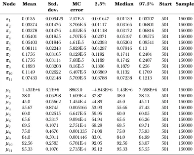
We can see the MC error and Mean for µ1 is too large that is over 0 to 100 of score’s interval. We conclude such case in which no students should be assigned to grade E. Besides, we have µ2 (i.e. mean for grade D) with lower bound of α / 2 = 0.025 is 37.87. Therefore, the instructor would decide to assign grade E if the raw scores of their students is less than 37. Conversely, grade D should be assigned for the scores between 37 and 43, grade D+ for scores greater than 43 and less than 53 and so on.
Furthermore, we have the probability of the raw scores belongs to the respective grades. For example, probability of the raw scores 96 are probably to be assigned grade A is about 0.0743 (or 7.43%), the raw scores of 70 will be assigned grade B- by the instructor with probability 0.1756 (or 17.56%) and so on as shown in Table 1. In addition, Table 2 demonstrates the minimum and maximum score for each letter grade and the percentage of students in the respective letter grade. We have about 25.81% of the students assigned to grade B- and approximately 79% of the students
Table 1 Optimal estimates of component means for first class
Node Mean Std. MC 2.5% Median 97.5% Start Sample dev. error
π1 0.0135 0.009429 2.57E-5 0.001647 0.01139 0.03707 501 150000
π2 0.03374 0.01476 3.706E-5 0.01117 0.03166 0.06801 501 150000
π3 0.03378 0.01476 4.052E-5 0.01118 0.03172 0.06816 501 150000
π4 0.05401 0.01855 4.707E-5 0.02371 0.05197 0.09575 501 150000
π5 0.05403 0.01846 4.61E-5 0.02393 0.05203 0.09541 501 150000
π6 0.08111 0.02243 5.829E-5 0.04297 0.07916 0.13 501 150000
π7 0.1756 0.03105 8.129E-5 0.1192 0.1741 0.2404 501 150000
π8 0.1756 0.03114 7.68E-5 0.1189 0.1742 0.2407 501 150000
π9 0.1893 0.03208 8.16E-5 0.1306 0.1879 0.256 501 150000
π10 0.1149 0.02622 6.407E-5 0.06869 0.1132 0.1709 501 150000
π11 0.07433 0.02148 5.709E-5 0.03788 0.07238 0.1213 501 150000
µ1 1.435E+6 3.2E+6 8863.0 –4.843E+6 1.43E+6 7.698E+6 501 150000
µ2 38.0 0.06298 1.609E-4 37.87 38.0 38.13 501 150000
µ3 45.0 0.05662 1.454E-4 44.89 45.0 45.11 501 150000
µ4 55.67 0.8745 0.005166 53.93 55.66 57.43 501 150000
µ5 60.0 0.02515 6.647E-5 59.95 60.0 60.05 501 150000
µ6 65.6 0.3317 9.094E-4 64.94 65.6 66.26 501 150000
µ7 69.5 0.1071 2.751E-4 69.29 69.5 69.71 501 150000
µ8 75.0 0.4676 0.001335 74.08 75.0 75.93 501 150000
µ9 84.0 0.5011 0.001446 83.01 84.0 84.99 501 150000
µ10 92.56 0.2583 6.781E-4 92.05 92.56 93.07 501 150000
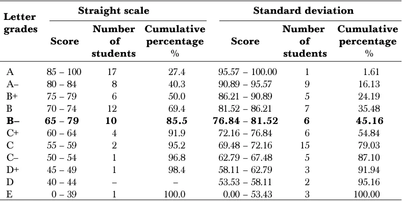
are passed. For comparison with the grades assigned by Straight Scale method and Standard Deviation method, see Table 3. Take an example of the pass grade is to be B-, that is approximately 86% of the student are passed. If the instructor applies the Straight Scale then the pass scores is 65 and above. While, if the instructor has decide to grade the student by the Standard Deviation method, then the pass score is 76.84 and 45.16% of the students will be passed.
Table 2 Minimum and maximum score for each letter grade, percent of students and probability of raw score receiving that grade for GB in the first class
Letter GB Number of Percentage Cumulative Probability grades From To student % percentage %
A 95 100 3 4.84 4.84 0.0743
A- 92 94 7 11.29 16.13 0.1149
B+ 83 91 10 16.13 32.26 0.1893
B 74 82 13 20.97 53.23 0.1756
B- 69 73 16 25.81 79.03 0.1756
C+ 64 68 5 8.06 87.1 0.0811
C 59 63 3 4.84 91.94 0.054
C- 53 58 2 3.23 95.16 0.054
D+ 44 52 2 3.23 98.39 0.0338
D 37 43 1 1.61 100 0.0337
E 0 36 0 0 100 0.0135
Table 3 Straight scale and standard deviation methods for the first class
Letter Straight scale Standard deviation
grades Number Cumulative Number Cumulative Score of percentage Score of percentage
students % students %
A 085 – 100 17 27.4 095.57 – 100.00 1 1.61 A– 80 – 84 8 40.3 90.89 – 95.57 9 16.13 B+ 75 – 79 6 50.0 86.21 – 90.89 5 24.19 B 70 – 74 12 69.4 81.52 – 86.21 7 35.48 B– 65 – 79 10 85.5 76.84 – 81.52 6 45.16 C+ 60 – 64 4 91.9 72.16 – 76.84 6 54.84 C 55 – 59 2 95.2 69.48 – 72.16 15 79.03 C– 50 – 54 1 96.8 62.79 – 67.48 5 87.10 D+ 45 – 49 1 98.4 58.11 – 62.79 3 91.94
D 40 – 44 – – 53.53 – 58.11 2 95.16
3.2 Second Case
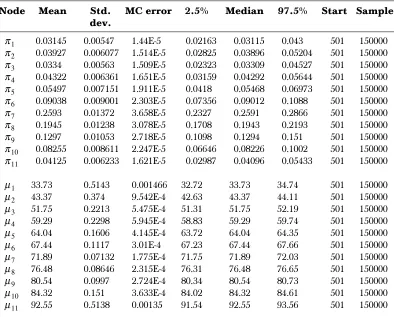
Now we have a class of 498 students. The mean is 71.53, the median is 73 and the standard deviation is 12.58. Table 4 shows WinBUGS output of the marginal moments and quantiles for means of each letter grade upon sampling. The updates for 150,000 Gibbs sampling took less than 2.5 minutes.
Table 4 shows the optimal estimate of component means and component probabilities of each letter grade. From Table 4, the instructor should assign grade A for the raw scores between 91 and 100, grade A- for the raw scores between 84 and 90, and so on. The corresponding grades intervals are decided from the credibility interval of 2.5% to 97.5% and with α = 0.05 (or α / 2 = 0.025). In addition, Table 6 shows the letter grades along with its score range for Straight Scale and Standard Deviation methods.
Compare Table 5 with Table 6 to the grades assigned by instructor. If the instructor decided the pass grade is B-. Then the percent of the students to be assigned for at
Table 4 Optimal estimates of component means for second class
Node Mean Std. MC error 2.5% Median 97.5% Start Sample dev.
π1 0.03145 0.00547 1.44E-5 0.02163 0.03115 0.043 501 150000
π2 0.03927 0.006077 1.514E-5 0.02825 0.03896 0.05204 501 150000
π3 0.0334 0.00563 1.509E-5 0.02323 0.03309 0.04527 501 150000
π4 0.04322 0.006361 1.651E-5 0.03159 0.04292 0.05644 501 150000
π5 0.05497 0.007151 1.911E-5 0.0418 0.05468 0.06973 501 150000
π6 0.09038 0.009001 2.303E-5 0.07356 0.09012 0.1088 501 150000
π7 0.2593 0.01372 3.658E-5 0.2327 0.2591 0.2866 501 150000
π8 0.1945 0.01238 3.078E-5 0.1708 0.1943 0.2193 501 150000
π9 0.1297 0.01053 2.718E-5 0.1098 0.1294 0.151 501 150000
π10 0.08255 0.008611 2.247E-5 0.06646 0.08226 0.1002 501 150000
π11 0.04125 0.006233 1.621E-5 0.02987 0.04096 0.05433 501 150000
µ1 33.73 0.5143 0.001466 32.72 33.73 34.74 501 150000
µ2 43.37 0.374 9.542E-4 42.63 43.37 44.11 501 150000
µ3 51.75 0.2213 5.475E-4 51.31 51.75 52.19 501 150000
µ4 59.29 0.2298 5.945E-4 58.83 59.29 59.74 501 150000
µ5 64.04 0.1606 4.145E-4 63.72 64.04 64.35 501 150000
µ6 67.44 0.1117 3.01E-4 67.23 67.44 67.66 501 150000
µ7 71.89 0.07132 1.775E-4 71.75 71.89 72.03 501 150000
µ8 76.48 0.08646 2.315E-4 76.31 76.48 76.65 501 150000
µ9 80.54 0.0997 2.724E-4 80.34 80.54 80.73 501 150000
µ10 84.32 0.151 3.633E-4 84.02 84.32 84.61 501 150000
least grade B- are 25.81%, 85.5%, and 45.16% respectively to the GB, Straight Scale and Standard Deviation method.
The results indicate that the grading plan via GB, Straight Scale and Standard Deviation method vary to the grades interval and the number of student getting the respective grade.
The implementation by WinBUGS package needs the instructor to decide the stopping point of the iterations. The stopping point shows an optimal parameter Table 5 Minimum and maximum score for each letter grade, percent of students and probability
of raw score receiving that grade for GB in the second class
Letter GB Number Percentage Cumulative Probability
grades From To of percentage
student % %
A 91 100 13 2.6 2.6 0.04125
A– 84 90 32 6.4 9.0 0.08255
B+ 80 83 64 12.9 21.9 0.1297
B 76 89 84 16.9 38.8 0.1945
B– 71 75 143 28.7 67.5 0.2593
C+ 67 70 53 10.6 78.1 0.09038
C 63 66 32 6.4 84.5 0.05497
C– 58 62 23 4.6 89.2 0.04322
D+ 51 57 16 3.2 92.4 0.0334
D 42 50 18 3.6 96.0 0.03927
E 0 41 20 4.0 100.0 0.03145
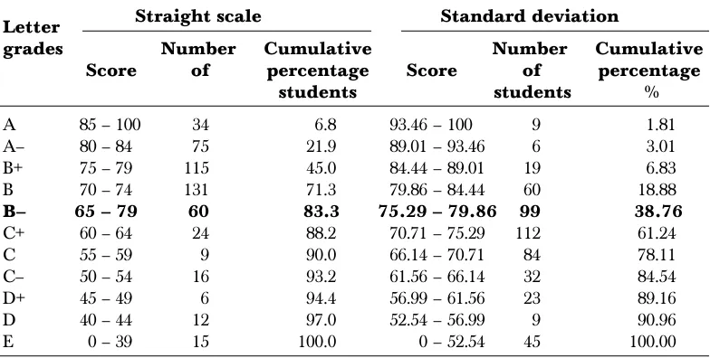
Table 6 Straight scale and standard deviation methods for the second class
Letter Straight scale Standard deviation
grades Number Cumulative Number Cumulative Score of percentage Score of percentage
students students %
A 085 – 100 34 6.8 93.46 – 100.0 9 1.81
A– 80 – 84 75 21.9 89.01 – 93.46 6 3.01
B+ 75 – 79 115 45.0 84.44 – 89.01 19 6.83 B 70 – 74 131 71.3 79.86 – 84.44 60 18.88 B– 65 – 79 60 83.3 75.29 – 79.86 99 38.76 C+ 60 – 64 24 88.2 70.71 – 75.29 112 61.24
C 55 – 59 9 90.0 66.14 – 70.71 84 78.11
C– 50 – 54 16 93.2 61.56 – 66.14 32 84.54
D+ 45 – 49 6 94.4 56.99 – 61.56 23 89.16
D 40 – 44 12 97.0 52.54 – 56.99 9 90.96
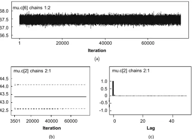
updates. One of the issues is at which updates the expected values converge to the optimal? Generally, there are three convergence tests; autocorrelation functions, Gelman-Rubin and traces diagnostics. For example see Figure 2. When the updates shows convergence, it means the expected values of parameter θ of the posterior density converges to E [p(θ/x)] with probability 1 as figured in Equation (3).
Figure 2(a) indicates that the traces diagnostics found the chains of sampling cover the same range and not shows any trend or long cycle, and in Figure 2(b) shows the 95th percentile of Gelman-Rubin scale reduction factor which measure between chain differences and rapidly approach to 1 if the sampler is close to the target distribution. Finally, we look at the autocorrelation function as in Figure 2(c). A long-tailed autocorrelation graph suggests that the model is ill conditioned and that the chains will converge more slowly [13]. The figure suggests convergences for all means and proportions of each letter grade. Results in Tables 1 and 4 show the stopping point or the convergence took 150 000 sampling.
Figure 2 a) Sampled values of means from one component, b) Gelman-Rubin convergence diagnostics and c) Autocorrelation of sample values
20000 44.5
44.0 43.5 43.0 42.5
3501 40000 60000
Iteration
(b)
20 1.0
0.5 0 -0.5 -1.0
0 40
Lag
(c)
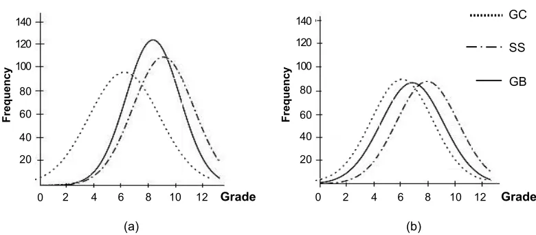
Figure 3 shows the plots of grade cumulative density function for Small Case and Large Case. The dotted line represents the cumulative distribution of Straight Scale and Standard Deviation methods and the smooth line is for grade according
mu.c[6] chains 1:2 68.0
67.5 67.0 66.5
1 20000
Iteration
60000
(a)
40000
to GB, whereas Figure 4 demonstrates the cumulative density plots for each letter grades along with its histograms.
3.3 Performance Measures
In measuring the performance, there are two measures to determine the performance of the grading methods. Refering to asymmetric loss and the absolute loss, we have decided to design the loss function in assigning letter grades as follows:
(
,)
,,
i i i i
i i i
i i i i
c y y y y
C y y
y y y y
− ≤
= − >
(4.3)
Figure 3 Cumulative distribution plots for SS, GC and GB grading methods
(a) (b) 14 Frequency Frequency 12 10 8 6 4 2 0 8.00 10.00 GB 12.00 6.00 4.00 2.00 0.00 140 120 100 80 60 40 20 0 8.00 GB 10.00 6.00 4.00 2.00 0.00 12.00
Figure 4 Density plots with histogram for the first and second class of GB method
Grade
0 2 4 6 8 10 12 140 120 100 80 60 40 20 Frequency Grade
where y is the numeric equivalent of the letter grade that the student truly deserves;
y is the numeric equivalent of the letter grade that the instructor assigned; and c is the positive constant that reflect instructor’s preference. This signify that, when c = 1, the instructors think equally badly about underestimating and overestimating the grade and when c > 1, the instructors think worse about underestimating than they think about overestimating and conversely if 0 < c < 1, the instructors think worse about overestimating than they think about underestimating. We introduce the class
loss (CC) as
1
1 n i i
CC C
n =
=
∑
. The lower CC means that the alternative grading methods assign grade closer to those actually assigned by the instructor. Another method in evaluating grading plan performance is by the raw coefficient of determination. Raw coefficient of determination is given by2
2 1
2
1
1
n i i
r n
i i
e R
y =
=
= −
∑
∑
where ei = yi – yi and 0≤Rr2 ≤1. Raw coefficient of determination is a measure of the variation of the dependent variable that is explained by the regression line and the independent variable. The value of R2 is usually expressed as a percentage and so it ranges from 0% to 100%. Thus, the closer the value is to 100%, the better the model is representing the data.
Table 7 shows that Rr2 for GB is higher than SS and GC. Therefore, a GB
method gets closer to the grades actually assigned by the instructor as compared to SS and GC method. However, between GB and SS, we can say there are no significant differences. But we can say GB and GC have significance difference of the high different in Rr2 value. In addition, the CC values for both lenient and neutral class
loss of GB are the lowest as compared to SS and GC. These results indicate that utilizing of GB method is better in assigning the letter grades instead of SS and GC methods.
^
Table 7 Performance of GB, straight scale and standard deviation methods
Neutral CC Lenient CC Rr2(%)
Straight scale (SS) 0.7903 1.2677 98.98
Standard deviation (GC) 1.4839 1.4839 93.71
4.0 CONCLUSION
The conditional Bayesian method is the method that allows for screening students accordingly to their performance relative to their peers and is useful for competitive circumstances where the feedback allow the students to compare their performance to their peers. Moreover, GB requires no fixed percentages in advance. Basically this method removes the subjectivity from Distribution Gap, making it more applicable. The conditional Bayesian grading reflects the common belief that a class is composed of several subgroups, each of which should be assigned a different grade. In this study, we have showed that conditional Bayesian grading successfully separates the letter grades. In applying conditional Bayesian method, the instructor needs to determine their own Leniency Factor. This is a spontaneous measure that reflects how lenient the instructor is when he or she grades their students performance.
ACKNOWLEDGEMENTS
The authors would like to thank the Faculty of Education, Faculty of Science and Universiti Teknologi Malaysia for the supports in this project.
REFERENCES
[1] Robert, L. W. 1972. An Introduction to Bayesian Inference and Decision. New York: Holt, Rinehart and Winston, Inc.
[2] Ebel, R. L. and D. A. Frisbie. 1991. Essentials of Educational. 3rd edition Englewood Cliffs, NJ.: Prentice-Hall, Inc.
[3] Martuza, V. R. 1977. Applying Norm-Referenced and Criterion-Referenced: Measurement and Evaluation.
Boston Massachusetts: Allyn and Bacon Inc.
[4] Merle, W. T. 1968. Statistics in Education and Psychology: A First Course. New York: The Macmillan Company.
[5] Stanley, J. C. and K. D. Hopkins. 1972. Educational Psychological Measurement and Evaluation. Englewood Cliffs, NJ.: Prentice Hall, Inc.
[6] Frisbie, D. A. and K. K. Waltman. 1992. Developing a Personal Grading Plan. Educational Measurement: Issues and Practice. Iowa: National Council on Measurement in Education.
[7] Pradeep, D. and G. John. 2005. Grading Exams: 100, 99, ... , 1 or A, B, C? Incentives in Games of Status. New Haven: Cowles Foundation Discussion Papers,Cowles Foundation, Yale University.
[8] Ash, R. B. 1972. Real Analysis and Probability. New York: Academic Press Inc.
[9] Robert, M. H. 1998. Assessment and Evaluation of Developmental Learning: Qualitative Individual Assessment and Evaluation Models. Westport: Greenwood Publishing Group Inc.
[10] Peers, I. S. 1996. Statistical Analysis for Education and Psychology Researchers. London: Falmer Press. [11] Congdon, P. 2003. Applied Bayesian Modeling. West Sussex, England: John Wiley & Son Ltd.
[12] Press, S. J. 2003. Subjective and Objective Bayesian Statistic: Principle, Models and Application. New Jersey: John Wiley & Son, Inc.
[13] www.mrc-bsu.cam.ac.uk/bugs/winbugswinbugswinbugswinbugswinbugs/contents.shtml. 2004. Hosted by the MRC Biostatistics Unit Cambridge, United Kingdom.
[14] Berger, J. O. 1985. Statistical Decision Theory and Bayesian Analysis. 2nd edition. New York: Springer-Verlag New York, Inc.
[16] Box, G. E. P. and G. C. Tiao. 1973. Bayesian Inference in Statistical Analysis. Massachusetts: Addison-Wesley Publishing Company, Inc.
[17] Casella, G. and E. I. George. 1992. Explaining Gibbs Sampler. The American Statistical Assosiation. 46(3): 167-174.
[18] Cornebise, J., M. Maumy, and G. A. Philippe. 2005. Practical Implementation of the Gibbs Sampler for Mixture of Distribution: Application to the Determination of Specifications in Food Industry. www.stat.ucl.ac.be/~lambert/BiostatWorkshop2005/ slidesMaumy.pdf.
[19] Figlio, D. N. and M. E. Lucas. 2003. Do High Grading Standards Effect Student Performance? Journal of Public Economics. 88(2004): 1815-1834.
[20] Gelman, A., J. B. Carlin, H. S. Stern, and D. B. Rubin. 1995. Bayesian Data Analysis. London: Chapman & Hall.
[21] Jasra, A., C. C. Holmes, and D. A. Stephens. 2005. Markov Chain Monte Carlo Methods and the Label Switching Problem in Bayesian Mixture Modeling. Statistical Science. 20(1): 50-57.
[22] Johnson, B. and L. Christensen. 2000. Educational Research: Chapter 5 -Quantitative and Qualitative Approaches. 2nd edition. Alabama: Allyn and Bacon Inc.