ABSTRACT
White, Katrina Elizabeth. Bioavailability of Polycyclic Aromatic Hydrocarbons in the Aquatic Environment.(under the direction of Damian Shea).
Polycyclic aromatic hydrocarbons (PAHs) are ubiquitous in the environment
and have been shown to elicit toxicity in humans and other organisms. Therefore, it
is important to monitor environmental concentrations of PAHs. Toxicologically, we
are concerned not only with the total PAH concentration but, with that fraction
available to partition into an organism (bioavailable fraction). This research fits
within three areas concerning bioavailability of PAHs including; 1) development of
methods to measure bioavailability in the field, 2) identification and characterization
of mechanisms controlling bioavailability and, 3) development of models to predict
bioavailability in the natural environment.
In the first phase of this research, the role of black carbon (BC) in the
bioavailability of PAHs in soil and sediment was examined by measuring sorption in
systems containing BC, natural organic matter (NOM), and microorganisms. A
model was developed to predict the bioavailable fraction of PAHs and factors that
may alter sorption in the natural environment from that predicted by laboratory
models were examined. In the second phase of this research, a novel passive
sampling device was developed to monitor truly dissolved PAH concentrations in
Sorption isotherms of pyrene-d10 were measured for diesel soot (DS),
Suwannee River NOM, Leonardite humic acids (HA), DS previously exposed to
NOM and HA, in binary systems containing both DS and NOM, and to DS exposed
to lake water. When DS was previously exposed to NOM, competition for sorption
sites was observed. However, when both pyrene-d10 and NOM were introduced to
DS simultaneously, less competition occurred and sorption was predicted within
92% of observed values using additive sorption models (based on the
unit-normalized Freundlich model and Polyani-Dubinin-Manes model). Weathering of DS
significantly reduced adsorption capacity but many strong sorption sites still
remained, possibly due to renewal of sorption sites by microorganisms. This
research demonstrated that sorption in the natural environment may be altered from
that predicted by laboratory models due to 1) competition of linear organic carbon for
sorption sites on DS, and 2) the presence of microorganisms. This research has
important implications for predicting bioavailability and ecotoxicological risk of
organic contaminants in soils and sediments.
In the second phase of this research, I evaluated a novel passive sampling
device, the polydimethyl(siloxane) (PDMS) integrative sampler, by 1) measuring the
uptake and release kinetics of 48 PAHs from water into PDMS 2) comparing
methods of loading performance reference compounds and 3) verifying the uptake
kinetics by comparing PAH concentrations predicted by samplers to measured
concentrations. Polycyclic aromatic hydrocarbons with a log Kow > 4.90 remained in
two weeks could be used for time-integrative monitoring of these compounds.
Compounds with a log Kow < 4.38 reach equilibrium rapidly (T50 < 9 d) and the linear
uptake model could not be used to predict analyte concentrations. Decreasing the
surface area to volume ratio of the sampler would easily solve this issue. Surface
area normalized sampling rates of PDMS samplers and semi-permeable membrane
devices (SPMDs), the most commonly used passive sampling device, were similar,
indicating that PDMS samplers are comparable to the SPMD. Concentrations of
PAHs in the PDMS samplers predicted concentrations in water within a factor of two
and on average within 30% of the actual concentration. Poly(dimethylsiloxane)
samplers offer great potential for monitoring PAH exposure in the aquatic
This dissertation is dedicated to:
My parents, Steve and Frances, who always believed in me and taught me I could
do whatever I set my mind to.
BIOGRAPHY
Katrina Elizabeth White was born on April 26th, 1975 in Emporia, KS and was the third child of Steve and Frances White. From the beginning she was fascinated
with animals and nature and enjoyed camping, canoeing, hiking, and playing in the
green house owned by her parents. She graduated a year early from Wichita High
School Metro Meridian.
She began her college career in 1992 at Kansas State University and
transferred to Wichita State University in 1994. It was here that she began her
career in science, pursued her love of animals, and developed a desire to find
answers to questions using scientific methods. She conducted research in the area
of animal behavior including topics such as selection tests of potential assistance
dogs, orangutan behavior, and reduction of repetitive behaviors of singly housed
hunting dogs. While she pursued a degree in psychology supporting her research in
animal behavior, she also pursued a degree in biology and took a course in
ecotoxicology. This course sparked her interest in environmental science and
toxicology and she decided to pursue a Ph.D. in this area. As an undergraduate
she was a Kansas McNair Scholar and had the opportunity to publish and present
her scientific work. In 1998, she completed a B.A. in psychology and in 1999 a B.A.
in biology. She entered the Ph.D. program at North Carolina State University in
2000, and under the direction of Damian Shea completed research in the area of
ACKNOWLEDGEMENTS
This work would not have been possible without the help and support of many
individuals. I would like to express my gratitude to my advisor, Damian Shea, for his
insight and advice on this research, constructive criticisms, aid in development of my
professional and writing skills, and for financial support. I would also like to thank
my committee members, W. Greg Cope, Chris Hofelt, and Elizabeth Guthrie Nichols
for their support, opportunities for teaching, scientific discussions, and review of my
dissertation. Special thanks to Pete Lazaro, who helped solve many issues with
equipment and taught me many of my analytical skills. S. Thorne Gregory
conducted microscopic analysis of diesel soot samples and Stephen Graham and
Cavell Brownie provided assistance in statistical analysis. I would also like to
acknowledge my fellow graduate students and laboratory members: Annette
McCarthy, Rebecca Heltsley, Wade Lehmann, Eun-ah Cho, Waverly Thorsen, Gail
Mahnken, and Robert Bringolf, as well as, the toxicology department administrative
TABLE OF CONTENTS
Page
List of Figures……….. xii
List of Tables……… xvii
List of Acronyms……….. xx
List of Nomenclature………... xxiii
Chapter 1. Review of Modeling Paradigms for the Sorption of Hydrophobic Organic Contaminants in Soil and Sediment ………. 1
Introduction ………. 2
Sediment Quality Guidelines ……… 3
Soil and Sediment ……….. 5
Organic Matter………. 6
Biogenic Origin……… 6
Humic Substances……….. 7
Kerogens and Coals………... 8
Pyrolysis Products……….. 8
Sorption………. 9
Absorption……… 10
Adsorption……… 11
Combined Models………... 18
Page
Discussion……… 23
References………... 24
Figures……….. 29
Tables……… 34
Chapter 2. Modeling Sorption of Polycyclic Aromatic Hydrocarbons to Diesel Soot, Natural Organic Matter, and Humic Acids……….. 36
Abstract………. 37
Introduction……….. 38
Materials and Methods………... 39
Materials………... 39
Isotherm Measurements……… 40
POM and PDMS Preparation and Extraction………. 41
KPOM and KPDMS Determination………. 41
Water Extraction……….. 42
Diesel Soot Extractions……….. 42
DOC, TOC, and BC……… 42
Specific Surface Area………. 42
Microscopic Analysis……….. 43
Sample Processing………. 43
Instrument Analysis and Quality Control………. 43
Page
Freundlich Model……… 44
Polyani-Dubinin-Manes Model……….. 45
Combined Models………... 46
Results and Discussion……….. 48
Sorption to POM and PDMS………. 48
Sorption to Diesel Soot……….. 48
Sorption to NOM and HA………... 49
Sorption to NOM Exposed DS……….. 50
Sorption to HA Exposed DS……….. 50
Sorption to Weathered DS………. 51
PDM versus Freundlich……….. 53
Modeling Sorption in Binary Systems……….. 54
Implications……….. 56
Acknowledgements………. 57
Supporting Information Available……….. 57
References………... 58
Figures……….. 63
Tables……… 67
Page
Chapter 3. Uptake Kinetics of Polycyclic Aromatic Hydrocarbons into Poly(dimethylsiloxane) Integrative Samplers from Water: An
Alternative Passive Sampling Device………... 85
Abstract………. 86
Introduction……….. 87
Uptake Model………... 89
Materials and Methods………... 92
Materials………... 92
Preparation of PDMS-IS………. 92
Uptake Exposure………. 92
KPDMS Determination………... 93
Loading Performance Reference Compounds………... 94
Elimination Exposures……… 94
Verification of Uptake Kinetics……….. 95
Sample Processing………. 95
Instrument Analysis and Quality Control………. 96
Data Analysis………... 97
Results……….. 98
Uptake and Release Kinetics……… 98
Loading PRCs onto Samplers………... 102
Verification of Uptake Kinetics. ……… 103
Page
Acknowledgement………... 107
Supporting Information Available……….. 107
References………... 108
Figures……….. 111
Tables……… 117
Supporting Information………... 125
Chapter 4. Comparison of Extraction Methods of Polycyclic Aromatic Hydrocarbons from Diesel Soot……… 129
Abstract………. 130
Introduction……….. 131
Materials and Methods………... 134
Materials………... 134
Soxhlet Extraction………... 134
Shaker Table Extraction………. 134
Ultrasonic Bath Extraction………. 135
Silica Column Clean Up………. 135
Experimental Design and Processing……….. 135
Instrument Analysis and Quality Control………. 136
Results and Discussion……….. 137
Extraction Methods………. 137
Page
Silica Column Clean Up……… 138
Accuracy………... 140
Molar Volume………... 141
Implications……….. 141
Acknowledgement………... 142
Supporting Information Available……….. 142
References………... 143
Figures……….. 146
Tables……… 147
Supporting Information………... 155
Chapter 5. Review of Fractionation Experiments of Soils and Sediments and Their Implications on the Factors Affecting Bioavailability of Polycyclic Aromatic Hydrocarbons……… 156
Introduction……….. 157
Grain Size………. 158
Density……….. 161
Specific Surface Area and Porosity……….. 164
Organic Carbon………... 167
Black Carbon……… 172
Discussion……… 179
References………... 182
Page
Appendix………... 190
1. Scanning electron micrographs of diesel soot from the
Environmental Protection Agency……… 191
2. Supplementary figures for research examining sorption to diesel
soot………. 194 3. Supplementary figures for research on the PDMS integrative
Sampler………. 198
LIST OF FIGURES
Page
Chapter 1. Review of Modeling Paradigms for the Sorption of Hydrophobic Organic Contaminants in Soil and Sediment.
Figure 1. Equilibrium partitioning theory………. 29
Figure 2. Comparison of the models used to estimate sorption of organic
contaminants in soil and sediment………... 30
Figure 3. Isotherms representing the traditional Freundlich model and the normalized Freundlich model. Normalization of the equilibrium concentration in water to SSC results in a collapse of isotherms to one plot. Data shown
[15] are from the Freundlich model applied to an aquitard material. Freundlich distribution coefficients were converted to K*F using K*F = KF
(SSC) nF……….. 31
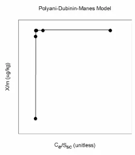
Figure 4. Representation of the Polyani-Dubinin-Manes model………. 32
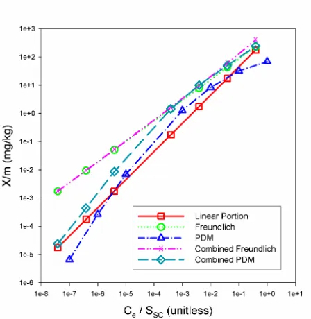
Figure 5. Comparison of the contribution of linear and nonlinear sorption for pyrene. The portion of linear sorption is calculated by CS = fOC KOC Ce,
where fOC = 0.012 and KOC = 104.16 (L/kg). Nonlinear sorption for the
Freundlich model is calculated using CS = fBC K*F (Ce/SSC)nF and for the PDM
model using CS = fBC Q’o x 10 (a’εSW/Vm)^b’ x ρ, where fBC = 0.0026, K*F = 105.24
(mg/kg), nF = 0.7309, Q’o = 101.3547 (cm3/kg), a’ = -0.0073, and b’ = 1.7802.
Combined models are the sum of linear and nonlinear sorption………. 33
Chapter 2. Modeling Sorption of Polycyclic Aromatic Hydrocarbons to Diesel Soot, Natural Organic Matter, and Humic Acids.
Figure 1. Isotherms of pyrene-d10 for POM (|) and PDMS (U)………... 63
Figure 2. Isotherms of pyrene-d10 and fitting of the Combined Freundlich model and Combined Polyani-Dubinin-Manes model to systems containing both diesel soot and natural organic matter. Data shown by { and solid line, Combined Freundlich model predictions shown by Uand dotted line, and the Combined Polyani-Dubinin-Manes predictions shown by and dashed-
Page
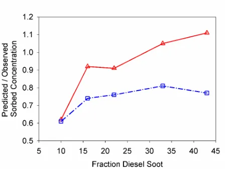
Figure 3. Comparison of the combined model predictions of sorbed concentrations / observed sorbed concentrations for pyrene-d10 by the fraction diesel soot. Combined Freundlich model predictions shown by U
and solid line, and the Combined Polyani-Dubinin-Manes predictions shown
by and dashed- dotted line……… 65
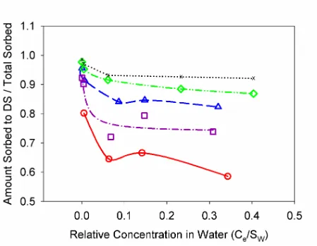
Figure 4. Fraction sorption of pyrene-d10 due to sorption to diesel soot in systems with diesel soot and natural organic matter, based on model
predictions. The fraction of diesel soot to total organic carbon is shown for: 9 ({ and solid line), 16 ( and dash-dot line), 22 (U and long dashed line),
33 ( and dash dot dot line), and 43 (X and dotted line)………. 66
Figure S1. Unit-normalized Freundlich model for pyrene-d10 applied to measured isotherms for EPA diesel soot, weathered diesel soot, and for EPA diesel soot with sorption to a linear phase considered. The estimated amount sorbed into fresh oil (U and dashed line) and weathered oil ( and solid line) was subtracted from the amount sorbed to EPA DS using Koil
values, the sum of PAHs as the mass of oil, and a mass balance. The
amount sorbed to an extractable organic phase was also considered……….. 76
Figure S2. Isotherms of pyrene-d10 for Suwannee River natural organic
matter and for diesel soot exposed to natural organic matter……….. 77
Figure S3. Unit-normalized Freundlich model for pyrene-d10 applied to measured isotherms for Leonardite humic acids and diesel soot exposed to
Leonardite humic acids at 2%, 20%, and 50% diesel soot: TOC……… 78
Figure S4. Polyani-Dubinin-Manes correlation curves for measured
isotherms of pyrene-d10 for EPA diesel soot, diesel soot exposed to NOM,
and weathered diesel soot………. 79
Figure S5. Polyani-Dubinin-Manes correlation curves of pyrene-d10 for measured isotherms of Leonardite humic acids and diesel soot exposed to
Leonardite humic acids at 2%, 20%, and 50% diesel soot: TOC……… 80
Figure S6. Sorption of pyrene-d10 predicted for EPA diesel soot exposed to Leonardite humic acids at 2%, 20%, and 50% diesel soot: TOC. Measured values shown by {and solid line. Predicted values (U and dashed line) were based on an additive model (q = fHA K*F, HA (Ce/SW) nF + fBC K*F, BC
(Ce/SW) nF) with the assumption that the fractions of humic acid (fHA) and
Page
Chapter 3. Uptake Kinetics of Polycyclic Aromatic Hydrocarbons into Poly(dimethylsiloxane) Integrative Samplers from Water: An
Alternative Passive Sampling Device.
Figure 1. Uptake curves of representative PAHs, fluorene ({),
phenanthrene (∆), and chrysene ( ), into PDMS-IS………. 111 Figure 2. Linear relationship between log Kow and log KPDMS. Data from the
KPDMS experiment ({ and solid line), an uptake experiment ( and dotted
line), and from Doong et al. (∆) are shown………. 112 Figure 3. Relationship between sampling rates and log Kow. Sampling rates
shown include uptake derived kes ({ and solid line), uptake derived Rss (∆
and dashed line), and elimination derived kes ( and dotted line).……… 113
Figure 4a. Ratio of freely dissolved PAH concentrations derived from PDMS-IS residues and the Rs to that measured in water in 3 laboratory
exposures. Experiment 1’s ({) PAH concentrations in water ranged from 360 - 570 ng/L while experiment 2 (∆) and experiment 3 ( ) PAH
concentrations ranged from 8 - 325 ng/L. Ratios for BaA (6.59 and 8.32), BaP (5.16 and 5.02), IN (17.82 and 9.30), and BghiP (6.93 and 5.27) in
experiment 2 and 3 respectively, are not shown……… 114
Figure 4b. Ratio of freely dissolved PAH concentrations derived from PDMS-IS residues and the uptake derived ke to that measured in water in 3
laboratory exposures. Ratios for BaA (8.9 and 11.5) in experiment 1 ({) and 2 (∆) and IN (4.9, exp. 1) are not shown. Experiment 3 ratios are
represented by ……… 115
Figure 5. Comparison of sampling rates of PDMS-IS ({) and SPMDs ()….. 116
Figure S1. Relationship between amount PAH taken up into a sampler and surface area for naphthalene ({), phenanthrene (∆), and benzo(ghi)perylene
( )………. 127
Figure S2. Relationship between the surface area to volume ratio and the time to reach 50% steady state (T50) for naphthalene ({), phenanthrene (∆),
Page
Chapter 4. Comparison of Extraction Methods of Polycyclic Aromatic Hydrocarbons from Diesel Soot.
Figure 1. Relationship between the mean relative extraction recoveries and molar volume of the smallest solvent used in each extraction method for
NIST DS and EPA DS……… 146
Appendix
Figure 1. Comparison of measured Ksoot values for unaltered diesel soot and
diesel soot previously exposed to natural organic matter………. 195
Figure 2. Linear relationships between log Kd and log KOW for unaltered
diesel soot, diesel soot previously exposed to natural organic matter, and
values measured by Jonker and Koelmans……… 196
Figure 3. Log Ksoot values measured in systems containing both diesel soot
and natural organic matter………. 197
Figure 4. Coefficients of variation of PAH concentration in water in
measurement of the uptake kinetics into PDMS integrative samplers………... 199
Figure 5. Measured PAH concentrations in water for select low molecular
weight PAHs in the uptake exposure of PDMS integrative samplers…………. 200
Figure 6. Measured PAH concentrations in water for select mid molecular
weight PAHs in the uptake exposure of PDMS integrative samplers…………. 201
Figure 7. Measured PAH concentrations in water for select high molecular
weight PAHs in the uptake exposure of PDMS integrative samplers…………. 202
Figure 8. Uptake curves of PAHs into PDMS integrative samplers.
Regressions shown for basic ke equation (blue line), ke equation with steady
state concentration based on KPDMS and CW-total (red line), ke equation with
steady state concentration based on KPDMS, CW-fd. and DOC of 80 mg/L
(green line), and ke equation with steady state concentration based on
KPDMS, CW-fd, and DOC of 2.6 mg/L (yellow dash-dot line). Figure shown on
next 9 pages………. 203
Figure 9. Elimination curves of PAHs from PDMS integrative samplers based on samplers loaded using the methanol method. Figure shown on
Page
Figure 10. Measured PAH concentrations in NIST diesel soot using different
extraction procedures………. 219
LIST OF TABLES
Page
Chapter 1. Review of Modeling Paradigms for the Sorption of Hydrophobic Organic Contaminants in Soil and Sediment.
Table 1. Factors affecting bioavailability of hydrophobic organic
contaminants……… 34
Table 2. Characteristics of different types of organic matter……….. 35
Chapter 2. Modeling Sorption of Polycyclic Aromatic Hydrocarbons to Diesel Soot, Natural Organic Matter, and Humic Acids.
Table 1. Summary of unit normalized Freundlich values for pyrene-d10……. 67
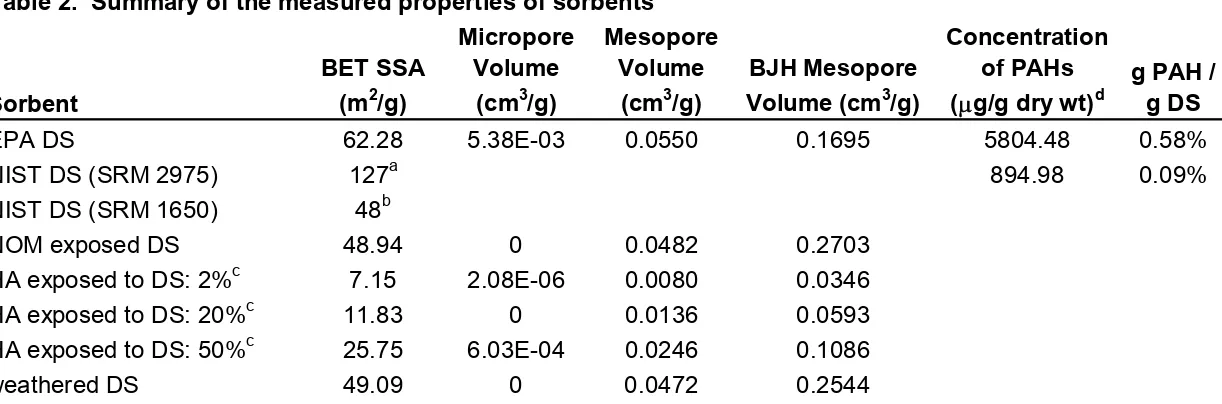
Table 2. Summary of the measured properties of sorbents……… 68
Table 3. Summary of predicted Kd values based on the unit normalized
Freundlich model for pyrene-d10 at high and low equilibrium concentrations
in water………. 69
Table 4. Summary of Ksoot values measured for PAHs native to diesel soot. 70
Table 5. Summary of Polyani-Dubinin-Manes model parameters for
pyrene-d10………. 72
Table S1. Summary of measured and published log KPOM and log KPDMS….... 82
Table S2. Physicochemical properties of pyrenea, used in calculations for
pyrene-d10……….. 84
Chapter 3. Uptake Kinetics of Polycyclic Aromatic Hydrocarbons into Poly(dimethylsiloxane) Integrative Samplers from Water: An
Alternative Passive Sampling Device.
Table 1. Polycyclic aromatic hydrocarbons analyzed in this study with
selected physico-chemical properties……….. 117
Table 2. Summary of measured uptake kinetics derived in an uptake
Page
Table 3. Summary of measured and published KPDMS and KMS………. 121
Table 4. Summary of exchange rate constants derived in elimination
studies……… 123
Table 5. Comparison of methods of loading PRCs………... 124
Chapter 4. Comparison of Extraction Methods of Polycyclic Aromatic Hydrocarbons from Diesel Soot.
Table 1. Relative extraction recoveries (%)a of extraction methods…………... 147
Table 2. Mean standard deviation (µg/g)a and coefficient of variationb for
each extraction method……….. 148
Table 3. Concentrationsa (mass fraction in µg/g dry weight) of PAHs in SRM
2975 diesel particulate matter determined using different extraction methods. 149
Table 4. Concentrationsa (mass fraction in µg/g dry weight) of PAHs in EPA
diesel soot determined using different extraction methods……….. 151
Table 5. Comparison of PAH concentrations (µg/L) in Alaska North Slope
crude oil with and without silica column clean up………... 153
Table 6. Ratio of measured PAH concentrations versus certified PAH
concentration in NIST SRM 2975 for different extraction methods………. 154
Table S1. Summary of surrogate internal standard recoveries for extraction
techniques……… 155
Table S2. Properties of solventsa used in extraction procedures……….. 155
Chapter 5. Review of Fractionation Experiments of Soils and Sediments and Their Implications on the Factors Affecting Bioavailability of Polycyclic Aromatic Hydrocarbons.
Table 1. Summary of fractionation studies included in review………. 186
Table 2. Variation in phenanthrene concentrations in water using different
Page
Table 3. Summary of observed relationships of sediment characteristics to
PAH bioavailability (degree of correlation listed in parenthesis1)………. 188 Table 4. Abbreviations of polycyclic aromatic hydrocarbons and selected
ACRONYMS
AEP fraction available for equilibrium partitioning
AOM amorphous organic matter
BC black carbon
BSAF biota sediment accumulation factor
CED cohesive energy density
CS combustible solids
CV coefficient of variation
DCM dichloromethane
DOC dissolved organic carbon
EPA Environmental Protection Agency
EPA DS diesel soot from the Environmental Protection Agency
FCV final chronic value
HOC hydrophobic organic contaminants
HSACM high surface area carbon materials
MDL method detection limit
MeOH methanol
MQL method limit of quantitation
MW molecular weight
NAPLs nonaqueous phase liquids
NIST National Institute of Standards and Technology
NIST DS diesel soot from the National Institute of Standards and Technology
OC organic carbon
PAHs polycyclic aromatic hydrocarbons
PC Piles Creek
PCB polychlorinated biphenyl
PDM Polanyi-Dubinin-Manes Model
PDMS poly(dimethylsiloxane)
PDMS-IS poly(dimethylsiloxane) integrative sampler
PFE pressurized fluid extraction
POM particulate organic matter
PRC permeability/performance reference compounds
PSD passive sampling device
PTFE poly(tetrafluoroethylene)
RER relative extraction recovery
SC soot carbon
SIS surrogate internal standard
SPMD semi-permeable membrane device
SQC sediment quality criteria
SRM standard reference material
TOC total organic carbon
NOMENCLATURE
a’ and b’ fitting parameters
b Langmuir site sorption affinity (L water µg sorbate-1)
Ce equilibrium concentrations of the solute in water, also
shown by CW
CO concentration in the organism (dry weight)
CPDMS(eq) concentration in PDMS at equilibrium
CPDMS (t) concentration in PDMS at time t
CPDMS-0 concentration in PDMS at time 0
CS sorbed concentration, also shown by q and X/m
CW concentration in water or pore-water, also shown be Ce
Cw-fd analyte concentration freely dissolved in water at steady
state
Cw-tot total analyte concentration in water
d exponent of adsorption isotherm; related to distribution of adsorption energies for gas phase sorption
d days
[DOC] dissolved organic carbon concentration
E characteristic energy of adsorption (J mol-1) = Eoβ
fBC fraction black carbon
ffd fraction analyte freely dissolved
flipid fraction lipid in organism (dry weight)
fOC fraction organic carbon or fraction organic carbon
fSC fraction soot carbon
fued fraction unavailable for equilibrium distribution
K*F unit-normalized Freundlich sorption coefficient
k1, k2, k3,
k4, and k5
empirical constants
KBC black carbon-water distribution coefficient
Kd solid-water distribution coefficient or sediment-water
distribution coefficient
KDOC dissolved organic carbon-water partition coefficient
ke exchange rate constant (d-1)
KF Freundlich distribution coefficient
KF,BC Freundlich black carbon distribution coefficient
Klipid lipid-water partition coefficient
KMS PDMS-solution partition-coefficient (mL/g)
KOC organic carbon – water partition coefficient
KOM organic matter normalized partition coefficients
KOW octanol-water partition coefficient
Kp partition coefficient
KPDMS PDMS-water partition coefficient (unitless)
KPOC particulate organic carbon-water partition coefficient
KS uptake clearance
ku uptake rate
Kx distribution coefficient for material x and water.
mM mass of one sampler (g)
N total amount of contaminant in the PSD
n number of samplers
nF Freundlich exponent
NM target amount per sampler
Nt total amount of analyte added to the system to get a
target amount per sampler
Po/P partial pressure (kPA or Pa)
[POC] concentration of particulate organic carbon
q mass adsorbed per amount sorbent, also shown by CS
and X/m
q’ adsorbed volume (m3)
q’max maximum adsorption capacity using volume, also
shown by QO’, and VO
qe’ adsorbed volume per unit mass of sorbent, also shown
by V/m
qL sorbed concentration due to linear sorption
qmax maximum site sorption capacity based on mass of
sorbate
qNL sorbed concentration due to nonlinear sorption
QO’ adsorption capacity at saturation based on volume
adsorbed
Rs effective sampling rates (L/d)
Rs-cm2 surface area normalized sampling rate
SA surface area
SA/V surface area to volume ratio (cm2/cm3) SS solid solubility in water (mol/ m3)
SSC subcooled liquid solubility
SW aqueous solubility (mol/L or mg/L)
T temperature (K)
t time in days or time of deployment
T50 time to reach 50% steady state
T90 time to reach 90% steady state
V/m volume of adsorbed molecules per mass sorbent, also shown by qe’
Vi intrinsic molar volume
Vm molar volume of sorbate
Vo maximum volume of sorbed chemical per unit mass of
sorbent, also shown by q’max, and QO’
VOM molar volume of the organic matter (L/mol)
VPDMS volume of PDMS (L)
VS volume solution (mLs)
X/m mass adsorbed per mass of sorbent
∆Sm sorbate entropy of melting
Ν normalizing factor of PDM model
α hydrogen-bonding donor parameter
β similarity coefficient or hydrogen-bonding acceptor parameter
βi ratio of adsorption energy between the sorbate and a
reference compound (Ε/Εο) βiΕo energy of adsorption
β∗ ratio of the characteristic adsorption energy in water versus gas (β∗=E
o,water / Eo, gas) ε differential work of adsorption
εSW adsorption potential in an aqueous system
γOM activity coefficient of the solute in water (mol/mol)
π∗ polarity/polarizability parameter
ρΟΜ density of organic matter (kg/L or g/mL)
CHAPTER 1
Introduction
Environmental acceptable concentrations of contaminants in the environment
are an important issue in the management of water, soil, and sediment. The
question of what concentration of a contaminant is safe is not straight forward, as
the total concentration in a media does not directly relate to toxicity. The toxicity will
be determined by the portion available for uptake or the bioavailable fraction, as it is
this fraction that may elicit toxicity. In soil and sediment, the bioavailable fraction
may be much lower than the total concentration measured because much of the
chemical may be sorbed to organic matter or other constituents of the sediment.
The fact that a portion of hydrophobic organic contaminants (HOC) may not
be bioavailable has been well documented. For example, the pattern of persistence
of many compounds in the environment shows an initial rapid rate of degradation
followed by a prolonged slow rate of degradation that may last for years or decades.
This is due to a decreased bioavailability of these compounds to the microorganisms
that degrade them. Regulatory agencies must therefore set environmental
acceptable concentrations based on the portion of contaminant available to an
organism. In order for this to be accomplished the bioavailability of HOCs must be
well understood. However, research on the bioavailability of contaminants in soil
and sediment has shown that there is a large variation in the bioavailable fraction
between different soils and sediments and which factors of bioavailability are the
Sediment Quality Guidelines.
In the 1990s, sediment quality guidelines were developed based on research
showing that organic matter was the primary sorbent of organic contaminants and
that toxicity was better predicted by sediment pore water HOC concentrations rather
than total sediment HOC concentrations (1). In other words, the truly dissolved HOC
concentration (e.g. pore water concentration in sediment) strongly correlated with
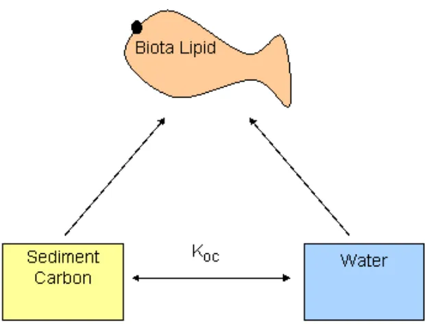
uptake and can be thought of as a measure of bioavailability (1). Equilibrium
partitioning theory provided a means to predict concentrations in pore water from
total sediment concentrations using partition coefficients (1,2). It predicts that
organic contaminants will primarily partition between organism lipid and sediment
organic carbon (OC) and will achieve equilibrium, so that concentrations in different
media may be predicted from the concentration in another media using partition
coefficients (Figure 1):
Kd = CS / CW =KOC fOC (1)
where Kd is the sediment - water distribution coefficient, CS is the sorbed
concentration in sediment, CW is the concentration in pore water, KOC is the OC –
water partition coefficient, and fOC is the fraction OC in sediment.
In equilibrium partitioning theory, HOC concentrations in pore water are
determined by solving equation 1 for Cw, and can be used to predict whether or not
HOC concentrations in sediments are acceptable by comparing Cw to water quality
concentrations in sediments and elicited response by normalizing CS to the fOC (1).
Di toro et al. (1) suggests that variation of a factor of two – three will remain.
However, a greater variation has been observed.
The biota-sediment-accumulation-factor (BSAF) was developed along with
sediment quality guidelines in order to estimate the body burden of a contaminant
from concentrations in sediment. The BSAF is a measure of bioconcentration rather
than bioavailability and takes into account metabolism and elimination. Biota
sediment accumulation factors can be calculated based on the following equation:
BSAF = CO / flipid / CS / fOC (2)
where CO is the concentration in the organism (dry weight) and flipid is the fraction
lipid in organism (dry weight). Theoretically, this BSAF would be equal to 1 (if you
assume that the lipid-water partition coefficient (Klipid) is equal to KOC or 2.3 (if the
octanol-water partition coefficient (KOW) = 0.41KOC) because the activity coefficient or
affinity of the chemical for lipid and OC is assumed to be approximately equal.
However, research shows that sorbents are present in the sediment with activity
coefficients not equal to lipid. Biota-sediment-accumulation-factors generally are
between 0 and 10 and have a much lower variability than bioconcentration and
bioaccumulation factors from water.
A large body of data has been collected that supports the equilibrium
partitioning model (1,3,4). However, over the past two decades several findings
Measured Kd valuesare often much greater than that predicted by organic matter
alone (5-14) and uptake by organisms exposed to the same total HOC concentration
in sediment is highly variable, even when normalized to fOC and flipid. The presence
of nonlinear sorption isotherms (15-19), fast and slow sorption domains (20,21),
competition (22), and a decreasing desorption and extractability with time (23)
indicate that a simple linear partitioning model is not adequate for modeling sorption
in complex systems containing heterogeneous organic matter with varying sorptive
properties. In this paper, components of sediment influencing bioavailability and the
models of sorption used to estimate bioavailability are reviewed. Bioavailability of
HOCs is controlled by physical, chemical, biological, and temporal factors (Table 1).
This paper will focus on recent research examining physical (characteristics of
sediment) and chemical processes that affect the bioavailability of HOCs.
Soil and Sediment
A basic understanding of the components of soil and sediment is necessary
to understand bioavailability. Sediment is composed of minerals (aluminosilicates,
oxides, and metals), inorganic particles, organic matter, interstitial water (pore
water), air, and nonaqueous phase liquids (NAPLs). Coarse sediments (sand and
gravel) are composed of large particles and are generally uncontaminated; in
contrast, fine sediments (clay, silt, mud) are made up of finer particles and in general
have a higher level of contamination. Aggregates in soils and sediment are formed
pores within soils and sediment that can alter the overall reactivity with
contaminants. In general, aggregate formation enhances water infiltration by
creating larger channels between particles (24).
Organic Matter
Soil and sediment organic matter is commonly defined as dead organic plant
and animal materials and their metabolites. They are macromolecules originating
from living organisms that have been altered through physical, chemical, and
biological processes. Organic matter in sediment exists as a continuum from newly
deposited materials derived from plant, animal, and microbial exudates, to
moderately aged humic substances, and finally geologically aged kerogen and coal.
In general, as organic matter ages (if it is not mineralized) it loses its functional
groups, becomes more aromatic, more persistent, and has higher partition
coefficients (25,26). It should be noted that aliphatic carbon is often present in aged
materials and may also exhibit high sorption coefficients (27).
Biogenic Origin
Organic matter of biogenic origin is the starting point of much of the organic
matter found in the environment and is made up of newly deposited plant and animal
parts such as leaves, roots, and other surface litter made up of carbohydrates, lignin,
proteins, lipids, and wood. In general, fresh organic matter is only a small portion of
the total organic matter as it will undergo decomposition processes and serve as the
Humic substances
Humus or humic substances are a heterogeneous mixture of decomposed
aliphatic and organic materials that are not identifiable as a specific biomass (i.e. the
parent molecule of plant parts, polysaccharides, proteins, and lignin) formed through
the process of humification (25). During humification, microorganisms convert OC to
CO2 to obtain energy while depositing nitrogen compounds. Their chemical
structure is poorly defined and they are commonly referred to as macromolecular
acids or oligoelectrolytes, that differ from the parent compounds by their relative
persistence (28). Humic substances are made up of amphiphiles (containing polar
and nonpolar groups) and they form micelles with their hydrophobic moieties
oriented toward the center and polar functional groups on the outside.
Humic substances may be chemically characterized based on their solubility
in acids and bases. Humic acids are soluble in basic solutions, fulvic acids are
soluble in both acidic and basic solutions, and humin are insoluble (29). Fulvic acids
tend to be yellow, have a low molecular weight, high percentage of polysaccharides
(up to 30%), a high number of functional groups (carboxylic and phenolic), and a low
aromatic content (Table 2) (25-28,30). Humic acids tend to be black, have a higher
molecular weight, fewer functional groups, and a higher aromaticity. They also
make up the majority of organic matter present in soils and sediments, with sediment
humic acids exhibiting sorption two-fold greater than that of soil (25,31). Humin, a
Kerogen and Coal
Kerogen and coal are produced through geological processes associated with
burial and increased temperatures that result in condensation. Kerogens are
disseminated carbon that is insoluble in non-oxidizing acids, bases, and organic
solvents (25). Others define it as organic matter that is insoluble in organic solvents
(25). These definitions would include coal and some fraction of humic substances.
Definitions that include base extraction eliminate humic and fulvic acids and acid
extraction would eliminate some of the humin (25). Kerogens are derived from
algae, residues of higher terrestrial plants (spores, pollen, cuticles, resins, and wax),
phytoplankton, and zooplankton. Kerogen releases petroleum hydrocarbons at
increased temperatures of 70 – 130oC (25). The type of kerogen (liptinite, exinite, vitrinite, and inertinite) may be identified through their reflectance and optical
characteristics (i.e. macerals).
While kerogen is dispersed, coals are sedimentary rock made up almost
completely of carbon. They are derived from cellulose, lignin, resins, spores, leaves,
and wood and are produced through peatrification and coalification involving
anaerobic degradation (25). They are composed of aromatic polymers, aliphatic,
aromatic hydrocarbons, and heterocompounds and considered a type of black
carbon (25). The glass to rubber transition temperature is about 330oC.
Pyrolysis Products
vegetation or fossil fuels and includes chars and soot. Chars are produced through
combustion of solid fuels and are carbonized residues of the starting material. Soots
are produced from particulate carbon that has recondensed from a gaseous phase.
It is made up of stacked aromatic sheets with many pores, a high surface area, and
is highly resistant to degradation.
Sorption
Sorption of organic contaminants to organic matter is one of the main factors
controlling bioavailability. There are two main types of sorption: absorption and
adsorption. Absorption involves an association or diffusion into a three-dimensional
matrix similar to a molecule diffusing into an organic solvent while adsorption
involves an association of a chemical onto a two-dimensional surface. In sediment,
a hydrophobic contaminant (sorbate) is commonly absorbed into organic matter
(sorbent). This process reduces the free energy of the sorbate remaining in an
aqueous solution. Absorption is linear, rapid, and does not exhibit competition. The
sorbate may also displace water molecules near a particle surface and adsorb to the
surface of that particle via van der Waals, dipole-dipole, induced-dipole,
hydrogen-bonding donor-acceptor interactions, London forces, and other weak intermolecular
interactions (32). Although these associations are weak when they exist between
two molecules, when many molecules interact simultaneously the van der Waals
interaction is additive and can be much stronger than interactions with pore water
example, if organic matter is dissolved in the water the tendency of HOCs to sorb to
sediment particles may be reduced because the unfavorable free energy of the
sorbate remaining in the water is reduced. Sorption is controlled by the sum of
these processes including the rate of sorption and the strength of intermolecular
interactions.
Chemicals freely dissolved in water are subject to processes such as
diffusion, volatilization, degradation, and uptake or diffusion into an organism.
These processes may to a large extent be excluded for chemicals associated with
particles or organic matter because these chemicals may be located at remote sites
within the particle or the activation energy of desorption may be high, making them
unavailable for diffusion. Chemicals associated with particles or organic matter are
subject to settling, re-suspension, deposition, uptake into an organism through
ingestion and subsequent desorption, and diffusion into another phase only if
desorption occurs.
Absorption
Chiou and Karickhoff laid the ground work for much of the research on
absorption in organic matter (34,35). They measured sorption of organic
compounds in sediments and soils over a range of concentrations in water and
found that overall isotherms were linear, directly related to the fOC, and independent
of other compounds (35). This indicated that sorption into OC was a function of
carbon-normalized or organic matter normalized partition coefficients (KOC or KOM) to
aqueous solubility (SW) and the KOW. Karickhoff found that the KOW was the best
predictor of KOC values (35).
This work was derived from linear-solvation-energy relationships (25).
Partition coefficients may be calculated, when the activity coefficient of the solute in
water is independent of concentration (i.e. up to the solubility limit) based on the
following equation:
KOM = 1/ γOM VOM ρΟΜ SW (3)
where γOM is the activity coefficient of the solute in water, VOM is the molar volume of
the organic matter, ρΟΜ is the density of organic matter, and SW is the aqueous
solubility. This equation shows that the KOM is inversely proportional to SW (log KOM
= a – b log SW) (33). However, for many nonpolar compounds the KOW is a better
predictor of the KOM, with the best regressions developed for compound classes
(10,25,37-42). Regressions have also been developed for specific environments.
For example, KOC’s of polycyclic aromatic hydrocarbons (PAHs) tend to be greater in
sediment than in soil and they tend to have a greater KOC than PCBs with similar
KOW (25). Allen-King et al. (25) provides a thorough review of this literature and
suggests that sorption for humic substances can be accurately predicted within a
factor of three using published regression equations for both SW and KOW. Adsorption
describe nonlinear sorption: the Langmuir and Freundlich equations (Figure 2).
Both of these models fit data on the mass adsorbed solute per amount sorbent (q or
X/m in µg/kg) over a range of equilibrium concentrations of the solute in a specified
medium (water for purposes of this paper, Ce in µg/L) at a constant temperature.
The Langmuir model assumes a defined number of sorption sites which can bind
one molecule and have a uniform energy of adsorption (Figure 2). It also assumes
that molecules on adjacent sorption sites do not interact. This implies that only a
monolayer of molecules may adsorb to the surface of the sorbent. In other words, at
high concentrations of solutes in water the amount sorbed to the sorbent becomes
constant due to saturation. Two constants are estimated in the Langmuir equation
(equation 4). The maximum site sorption capacity (qmax in µg sorbate/kg sorbent) is
the concentration sorbed when one monomolecular layer occurs. The Langmuir site
sorption affinity (b in L water/ µg sorbate) is a constant related to the heat of
adsorption (43).
q = b qmax Ce / (1 + b Ce) (4)
The Freundlich model assumes that q may continue to increase with
increasing solute concentrations in water and is not constrained to a monolayer
(Figure 2). Although it is physically impossible for q to continuously increase, most
relevant systems are dilute enough that this area of the curve is not approached
(44). This model also assumes that the energy of adsorption distribution for
the Freundlich equation are the Freundlich distribution coefficient (KF) and the
Freundlich exponent (nF) (equation 5). Steep slopes (nF near 1) indicate that the
adsorptive capacity is high at high Ce and rapidly decreases at low Ce. Flat slopes
(nF << 1) indicate that adsorptive capacity is only slightly reduced at low Ce.
q = KF CenF (5)
The Freundlich model has consistently been shown to describe sorption of
organics to BC (6,45-47). The model accounts for the expected variability in
adsorption energies among sorption sites and does not constrain sorption to a
monolayer. It is not expected that sorption sites on environmental BC are uniform in
adsorption energies or that only a monolayer of sorption will occur. However, the
Langmuir model does allow for an estimation of the number of sorption sites
available and also fits isotherm data for many BC materials. Cornelissen and
Gustafsson (45) measured isotherms for combusted sediment and used the
Langmuir model to estimate when saturation of BC would occur. Use of the
Langmuir model allows for estimation of the q value in which sorption will transition
from sorption to BC to sorption to other PAHs or organic matter bound to BC.
In very dilute systems, b Ce becomes so small that it can be neglected and
the Langmuir equation can be reduced to the equation for a distribution coefficient:
KBC = q / Ce = b qmax (6)
values measured at less than 1% the solubility of the compound (48). The Langmuir
affinity was estimated based on the following equation:
b = 1 / Ss exp (∆Sm – 15 J/(mol K)) / R (7)
where SS is the solid solubility in water in mol/m3, ∆Sm is the sorbate entropy of
melting, and R is the ideal gas constant.
Carmo et al. (49) showed that the units of KF vary nonlinearly with nF (49).
This results in inaccurate comparisons of KF values for different sorbents (49). They
proposed using a solubility-normalized Freundlich isotherm based on a relative
concentration shown in equation 8:
q = K*F (Ce / SW)nF (8)
where K*F is the unit-normalized sorption coefficient and represents the mass
adsorbed when saturation is approached (49). This equation converges isotherms
for various compounds to the same material to a single isotherm due to sorption
components being inversely proportional to SW according to Raoult’s Law (Figure 3)
(25). At high concentrations and when linear sorption dominates, K*F/fOC is equal to
the compound solubility in organic matter (25).
Many researchers recognize that adsorption models derived from the Polanyi
adsorption potential for gas phase adsorption (equation 9) are the most powerful for
modeling adsorption to sorbents with heterogeneous surfaces (50):
where ε is the differential work of adsorption, Po/P is the partial pressure, and T is
the temperature. In this model, the volume of adsorbed molecules per mass sorbent
(V/m) (the mass adsorbed per mass of sorbent can be converted to V/m using
density) is plotted against the differential work of adsorption (RT ln (Po/P)) to form a
characteristic curve (50). Alternately, a correlation curve may be constructed by
replacing the differential work of adsorption with T/V log Po/P (50). This model assumes that there is a fixed adsorption space around the adsorbent with the
primary mechanism of adsorption being van der Waals forces or London forces for
gases and vapors (32,50). All sorbates on a given sorbent will have a common
limiting volume at zero adsorption potential and these adsorption potentials are
related to each other by constant characteristic factors (50). Therefore, isotherm
curves for a given sorbent will collapse when an appropriate divisor (often a
normalizing factor (Ν) is used) that accounts for differences in molecular size (50).
The Dubinin and Ashtakhov equation, developed for gas and porous structures is fit
to the above curve:
q’ / q’max = exp [-(R T ln (Po / P)/ βi Εo)d] (10)
where q’ is the adsorbed volume, q’max is the maximum adsorption capacity, βiΕo is
the energy of adsorption, with βi as the ratio of adsorption energy between the
sorbate and a reference compound (ε/εο), and Εοis the energy of adsorption for the
reference compound. The exponent d is a fitting parameter. Manes suggests that
the βiΕo may be estimated from the molar volume of the sorbate (Vm) with a
Manes and coworkers extended this model to be used in aqueous systems
with the primary difference being that the sorbate must displace an equal volume of
water on the sorbent (51). The Polanyi-Dubinin-Manes adsorption potential (εSW) is
the work or free energy required for a molecule to move from bulk solution to the
adsorption space and varies with solution concentration (32):
εSW = R T ln (SW / Ce) (11)
Manes suggests that when compounds exist in the solid state or crystalline state
under ambient temperatures, they will have a reduced packing efficiency. Replacing
SW with the subcooled liquid solubility of the compound (SSC) would move isotherms
closer to that of liquid chemicals (25). However, energy differences between
adsorption as a solid and adsorption as a liquid are overestimated by the heats of
fusion and many researchers still use the SW (16,50,52) . The free energy ranges
from a maximum value, when the adsorbed volume is low, to zero, when the
concentration reaches the solubility limit or the adsorbed volume reaches its
capacity (32). The Polanyi-Dubinin-Manes Model (PDM) equation describes
nonlinear sorption in aqueous systems by replacing ln (Po/P) with ln (SW/Ce):
q’ = q’max exp [-(R T ln (SW / Ce)/ βi β∗ Eo)d] (12)
where β∗ is the ratio of the characteristic adsorption energy in water versus gas (β∗=
Eo,water / Eo, gas). This model predicts the same adsorbed volume for all chemicals
with similar abscissa and that this can be determined by Ce/SW and the chemicals
affinity, βiβ∗Eo (25). Accordingly, βiβ∗Eo may be replaced by a normalizing factor
βiβ∗Eo and successfully fit multiple compounds (benzene, chlorobenzenes, and
PAHs) to a characteristic curve for an aquitard material using the following equation
(16):
log (qe’) = log (QO’) + a’ (εSW / Vm)b’ (13)
where qe’ is the adsorbed volume per unit mass of sorbent (cm3/kg), QO’ is the
adsorption capacity at saturation (cm3/kg), and a’ and b’ are fitting parameters (the ‘ distinguishes between volume (qe’) and mass (qe) of the sorbate) (Figure 4). This
successfully collapsed isotherms for sorbates that were liquids but not solids, which
tend to have a lower adsorption capacity (16). They did not use the subcooled liquid
solubility for solid compounds (which would result in moving the solid isotherm closer
to that of liquids) because the heat of fusion for the chemicals in question were all
much higher than the energy differences between adsorption as a solid and
adsorption as a liquid (calculated as 2.3 RT log SSC/SS) (16). They suggest the
reduced maximum adsorption capacity for solid chemicals is due to a decreased
packing efficiency within micropores (16) and that the fit of the PDM model to their
aquitard material suggests that sorption is the result of pore filling onto a high
surface area carbon material (16).
Crittenden et al. (32) developed a method of estimating Ν based on
adsorption energy, interaction energy between organic sorbate and adsorbent,
interaction energy between water and the adsorbent, interaction energy between
adsorbed molecules, the interaction energy between organic and water molecules,
following equation for Ν:
Ν = k1 Vi/100 + k2 π∗ + k3 β + k4 α + k5 (14)
where k1, k2, k3, k4, and k5 are empirical constants, 100 is a scaling factor, Vi is the
intrinsic molar volume, π∗ is the polarity/polarizability parameter, β is the
hydrogen-bonding acceptor parameter, and α is the hydrogen-hydrogen-bonding donor parameter.
Crittenden et al. (32) applied this method to 56 organic compounds and 8 sorbents
(mainly activated carbon materials) and found a common isotherm.
Kleinedam et al. (51) successfully used the following form of the PDM model
to describe sorption onto to various carbon materials:
CS = Vo ρο exp [-R T(-ln Ce / SW)/ E]b (15)
where VO is the maximum volume of sorbed chemical per unit mass of sorbent
(cm3/kg), and ρο is the compounds density (g/cm3). In this equation, the only fitting
parameters are VO and E.
The exponent b is comparable to the d exponent and is dependent on the
distribution of the adsorption energy. It is often set to a predefined number (1-5)
based on characteristics of the sorbent, for example the Dubinin-Radushkevich
equation uses a value of 2 (51). Manes suggests that predefining d was originally
performed for convenience in converting curves to a straight line and that a
predefined value is no longer needed.
Combined Models
Two basic concepts have been used to describe the dual mode sorption
polymer theory views organic matter as a polymer which may exist in either a soft,
rubbery like state (temperature is above the glass transition temperature) or a hard
glassy state (temperature is below the glass transition temperature). Sorption into
organic matter in the soft or rubbery state is assumed to be linear and for the hard or
glassy state, nonlinear. The other theory relies on the heterogeneity of organic
matter and suggests that linear sorption will occur for the fulvic and humic acids with
the isotherm becoming more nonlinear for high surface area carbon materials such
as kerogen, coal, and pyrolysis products. Whichever theory is used, it is understood
that both linear and nonlinear sorption should be accounted for. It is likely that both
theories are important in understanding the overall sorption process in sediments.
However, recently the importance of high surface area carbon materials (HSACM) in
nonlinear sorption has been clearly demonstrated (6,10,45,47,53-57). Allen-king et
al. (25) suggest that 1) the absorption portion of the curve can be approximated
within a factor of three based on the large body of literature available, 2) the largest
deviations from the absorption model will occur at low aqueous concentrations and
will be due to thermally altered carbon materials, and 3) the crossover point from
adsorption dominated isotherms to absorption dominated isotherms depends on the
strength of the sorbent and the relative amount of the adsorption sorbent present in
comparison to the amount of sorbent exhibiting absorption behavior.
The majority of combined models assume that sorption is additive, that is, a
sum of the nonlinear and linear sorption curves.
where qL is the sorbed concentration due to linear sorption and qNL is the sorbed
concentration due to nonlinear sorption. The linear model has been combined with
the Freundlich, Langmuir, and PDM models with variations in whether the fOC and
fraction BC (fBC) are considered (Figure 5). For the purposes of this review, these
models will be referred to as combined models based on the method used to model
nonlinear sorption.
Bucheli and Gustafsson (6) suggested that Kd in sediments should be
estimated based on sorption to both OC and soot carbon:
Kd = fOC KOC + fSC KSC (17)
where fSC is the fraction soot carbon and KSC is the soot carbon-water distribution
coefficient. The fOC and fSC or fBC is estimated from the total OC (TOC), where fOC is
the fraction OC exhibiting linear sorption and fBC is the fraction exhibiting nonlinear
sorption and they add up to the TOC. This equation does not account for the fact
that the KSC is dependent on the Ce.
Accardi-Dey and Gschwend (46) expanded this model to account for the
nonlinear sorption onto BC materials:
CS = fOC KOC Ce + fBC KF,BC CenF (18)
where KF,BC is the Freundlich distribution coefficient for BC. The Kd can then be
estimated based on the following equation:
Kd = fOC KOC + fBC KBC CenF-1 (19)
This equation was successful in predicting Kd values of PAHs, polychlorinated
and estimating body burdens and pore-water concentrations in marine sediments
(59).
The Langmuir model has also been used to model sorption in combined
models (19).
CS = KOC Ce + b qmax Ce / (1 + b Ce) (20)
Huang et al. (19) applied this model for phenanthrene to 27 different soils and
sediments and found it fit the data well.
Xia and Ball (16) developed a combined model based on the PDM model:
q = QO’ x 10a’(εSW /Vs)b’ x ρο +Kp Ce (21)
In this model, q is plotted against the adsorption potential density (εSW/Vm) and a’, b’,
q’max, and Kp (OC-water partition coefficient) are the fitting parameters (16). This
model successfully predicted sorption of 9 compounds to an aquitard material (16).
Other researchers have also used a combined PDM model but added a
parameter for the fOC (51,52). For example, Kleinedam et al. (51) used the following
equation.
CS = Vo ρο exp [-R T(-ln Ce / SW) / E]b + fOC Kp Ce (22)
In this model, Kp was estimated based on KOC values and Vo and E are the only
fitting parameters for the nonlinear part of the isotherm. They found that the
subcooled liquid solubility rather than water solubility tended to have a better fit and
used this model to describe sorption of five organic compounds to nine sorbents (51).
Finally, Cornelissen and Gustafsson (60) developed a combined Freundlich
unburned coal:
CS = fOC KOC Ce + fBC KF,BC CenF,BC + fCC KF,CC CenF,CC (23)
where CC designates the parameters for coal carbon.
Competition
All of these models fail to account for the expected competition present in the
environment. Zhao et al. (22) developed a competitive dual mode model based on
the Langmuir model and successfully predicted sorption of phenanthrene,
anthracene, and pyrene to sediment. The PDM model has also been developed to
account for competition and this is reviewed well by Manes (50).
I hypothesize that OC exhibiting linear type sorption (hereafter referred to as
linear OC) may act as both a sorbent and a sorbate onto OC exhibiting nonlinear
sorption (hereafter referred to as nonlinear OC). This is supported by the work of
Cornelissen and Gustafsson (45) who measured sorption of phenanthrene to original
sediment, sediment stripped of native sorbates (containing linear OC and BC), and
combusted sediment (containing only BC). At low aqueous concentrations
phenanthrene sorption to combusted sediment exceeded the sorption to the original
sediment and sediment stripped of native sorbates, indicating that native
contaminants and/or OC competed for sorption sites on the BC. They calculated an
environmental KF,BC that was lower than the intrinsic KF,BC by a factor of nine (45).
With this in mind, a good model would need to consider the ratio of linear
OC/nonlinear OC with a factor to estimate when saturation of nonlinear OC occurs
sorbates (for example PAHs native to diesel soot) may also need to be treated as
both sorbates onto nonlinear OC and sorbents for further sorption of other organic
contaminants. This is supported by Hong et al. (61) who found that lampblack (a
type of BC) containing high levels of PAHs exhibited sorption similar to that of a coal
tar mixture due to saturation of sorption sites on the lampblack.
Discussion
All of these models have been used in the literature to estimate sorption of
organic contaminants to soils, sediments, and BC materials with the combined
Freundlich model and the combined PDM model being the most widely used. Both
of these models have advantages and disadvantages. For example, the combined
Freundlich model is the easiest to use but the units of KF are not linearly related to nF.
The combined PDM model allows for the estimation of sorption parameters at
various temperatures and for other compounds but it is difficult to estimate Ν. Xia
and Ball’s (16) method of estimating PDM parameters using the molar volume has
significantly reduced this complication. The prominent questions that are being
debated are 1) whether to use the SW or the SSC for normalization of Ce, 2) which
model is most appropriate for modeling sorption across many sediments and soils 3)
how to account for competition, and 4) how to account for linear OC acting as a
sorbate and sorbent. Future research should test a combined normalized Freundlich
model and a combined PDM model that incorporates fBC. It should also examine
how linear OC may alter sorption on BC materials from that predicted by laboratory
References
(1) DiToro, D. M.; Zarba, C. S.; Hansen, D. J.; Berry, W. J.; Schwartz, R. C.; Cowan, C. E.; Pavlou, S. P.; Allen, H. E.; Thomas, N. A.; Paquin, P. R. Environ Toxicol Chem1991, 10, 1541-1586.
(2) Ronday, R.; Van Kammen-Polman, A. M. M.; Dekker, A.; Houx, N. W. H.; Leistra, M. Environ Toxicol Chem1997, 16, 601-607.
(3) Ferraro, S. P.; II, H. L.; Ozretich, R. J.; Specht, D. T. Arch Environ Contam Toxicol1990, 19, 386-394.
(4) Tracey, G. A.; Hansen, D. J. Arch Environ Contam Toxicol1996, 30, 467-475.
(5) Gustafsson, O.; Gschwend, O. M. Aquatic phase-distributions of hydrophobic chemicals not predictable from organic matter partitioning models. In Bioavailability of Organic Xenobiotics in the Environment; Baveye, P., Block, J. C., BGoncharuk, V., Eds.; Kluwer Scientific: Amsterdam, The Netherlands, 1999; pp 327-348.
(6) Bucheli, T. D.; Gustafsson, O. Environ Sci Technol2000, 34, 5144-5151.
(7) Gustafsson, O.; Gschwend, P. M. Phase distributions of hydrophobic
chemicals in the aquatic environment. In Bioavailability of Organic Xenobiotics in the Environment: Practical Consequences for the Environment; Block, J. C., Baveye, P., Goncharuk, V. V., Eds.; Kluwer Academic Publishers: Boston, MA, 1999; pp 327-348.
(8) Kraaij, R.; Seinen, W.; Tolls, J.; Cornelissen, G.; Belfroid, A. C. Environ Sci Technol2002, 36, 3525-3529.
(9) Mcgroddy, S. E.; Farrington, J. W. Environ Sci Technol1995, 29, 1542-1550.
(10) Bucheli, T. D.; Gustafsson, O. Environ Toxicol Chem2001, 20, 1450-1456.
(12) Maruya, K. A.; Risebrough, R. W.; Horne, A. J. Environ Sci Technol1996, 30, 2942-2947.
(13) Muller, S.; Wilcke, W.; Kanchanakool, N.; Zech, W. Soil Sci2000, 165, 412-419.
(14) Gustafsson, O.; Gschwend, P. M. Soot as a strong partition medium for polycyclic aromatic hydrocarbons in aquatic systems. In Molecular Markers in Environmental Geochemistry; Eganhouse, R. P., Ed.; American Chemical Society: Washington DC, 1997; pp 365-381.
(15) Kleineidam, S.; Rugner, H.; Ligouis, B.; Grathwohl, P. Environ Sci Technol 1999, 33, 1637-1644.
(16) Xia, G.; Ball, W. P. Environ Sci Technol1999, 33, 262-269.
(17) Karapanagioti, H. K.; Kleineidam, S.; Sabatini, D. A.; Grathwohl, P.; Ligouis, B. Environ Sci Technol2000, 34, 406-414.
(18) Chiou, C. T.; McGroddy, S. E.; Kile, D. E. Environ Sci Technol1998, 32, 264-269.
(19) Huang, W.; Young, T. M.; Schlautman, M. A.; Hong, Y.; Weber, W. J. Environ Sci Technol1997, 31, 1703-1710.
(20) Pignatello, J. J.; Xing, B. Environ Sci Technol1996, 30, 1-11.
(21) Shor, L. M.; Rockne, K. J.; Taghon, G. L.; Young, L. Y.; Kosson, D. S. Environ Sci Technol2003, 37, 1535-1544.
(22) Zhao, C.; Hunter, M.; Pignatello, J. J.; White, J. C. Environ Toxicol Chem 2002, 21, 2276-2282.