Adaptive Frameless Rendering.

(1)

ABSTRACT

SRINIVASAN, ABHINAV. Adaptive Frameless Rendering. (Under the direction of Benjamin Watson.)

(2)

(3)

Adaptive Frameless Rendering

by

Abhinav Srinivasan

A thesis submitted to the Graduate Faculty of North Carolina State University

in partial fulfillment of the requirements for the Degree of

Master of Science

Computer Science

Raleigh, North Carolina

2016

APPROVED BY:

Christopher Healey John Turner Whitted

(4)

DEDICATION

(5)

BIOGRAPHY

(6)

ACKNOWLEDGEMENTS

I would like to thank my mother, my father, and my brother, for their constant support and encouragement.

I would also like to thank Sri Sankara Senior Secondary School - the school that I considered home for a decade, and the school that adopted me as one of its own. I would like to thank SASTRA University - the institution that shaped my outlook and instilled passions in me that I would not have been able to discover elsewhere. I would also like to thank North Carolina State Univeristy for giving me an opportunity to pursue academic excellence, and for helping me find strength in the wolfpack.

I would also like to extend my gratitude to Dr Benjamin Watson for giving me the wonderful opportunity to work on a project that was simultaneously challenging and exciting. His constant words of encouragement and his mentorship brought forth the best I had within myself. I would also like to thank Dr Christopher Healey and Dr John Turner Whitted for consenting to being a part of my thesis committee.

I would like to thank all of my friends for being companions with me on this truly marvelous journey. I would especially like to thank Adam Marrs, on whom I have relied on whenever the magnitude of the obstacles that I’ve faced have overwhelmed me. His persective and inputs have been invaluable to me and were a critical component in this project.

(7)

LIST OF TABLES

Table 3.1 Pseudocode . . . 28

(9)

LIST OF FIGURES

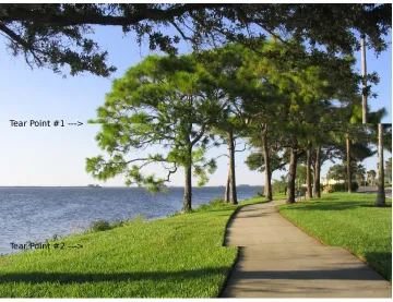
Figure 2.1 Image Tearing (courtesy Wikipedia) . . . 4 Figure 2.2 A depiction of single, double, and triple buffering courtesy of [6]. In

single buffering, the front buffer is always shown. In double buffering, one buffer is the front buffer, and the other the back buffer. These two buffers swap positions for each frame. In triple buffering, an additional pending buffer is present. In triple buffering, a buffer is first cleared, and rendering to it is begun (pending). Second, the system continues to use the buffering for rendering until the image has been completed (back). Finally, the buffer is shown (front). . . 6 Figure 2.3 Motion Blur in Frameless Rendering . . . 8 Figure 2.4 Practically Frameless Rendering remaps how frame-buffer pixels are

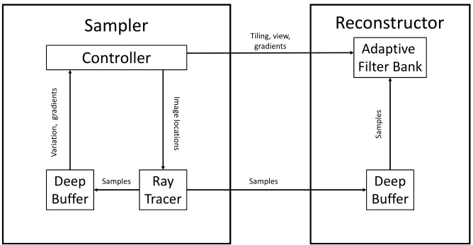
displayed. Image courtesy [24] . . . 9 Figure 3.1 System Components . . . 12 Figure 3.2 Tiles cluster around edges and areas of motion, thereby biasing the

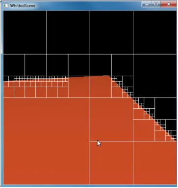
sampling towards that region. To prevent tiles from getting too big or too small, and thereby skewing sampling too much, it is also reasonable to restrict the maximum and minimum sizes that tiles can take. For example, the bottom left corner of this image is occupied by one very big tile. If a new object were to appear there, then it takes longer to capture the variance in that region. . . 14 Figure 3.3 Because tiling is biased towards edges and areas of motion, that is

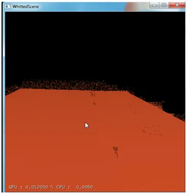
where sampling takes place too. In this picture, new samples are marked by a green pixel. So it’s clear that towards the edges, where the spatio-temporal variance is high, more samples are taken. And in regions with low variance, such as plain surfaces and background, very few samples are taken. . . 15 Figure 3.4 Crosshairs, which are stored in the deep buffer, are using to calculate

the gradients. We used the symmetrical crosshairs initially, but have since modified the implementation to use the tetrahedron crosshairs. Previous of adaptive frameless rendering by [10] have used the sym-metrical crosshairs. . . 17 Figure 3.5 Pixie dust as seen in traditional frameless rendering. A characteristic

(10)

Figure 3.6 Adaptive Reconstruction. At static moments, the difference between traditional and adaptive reconstuction is minute. However, once the scene becomes dynamic, then adaptive reconstruction gives a much better quality image than the traditional counterpart. This figure shows adaptive reconstruction at a dynamic moment. Notice how the pixie dusts at the trailing edge have become significantly blurred. . . 22 Figure 3.7 A sampling density map (left) is used by the reconstructor to determine

the expected local sample volumeVsand the tile gradients (right)Gx,

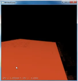
Gy, and Gt. Here, Gx, Gy, and Gt are shown in blue, green, and red, respectively. . . 23 Figure 4.1 Adaptive Frameless Rendering on a simple, one plane scene. The

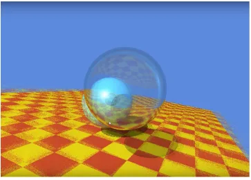
pic-ture on the left shows the scene during a still moment, and the picpic-ture on the right shows the scene when there is motion. . . 30 Figure 4.2 Adaptive Frameless Rendering on a more complex scene. The picture

(11)

Chapter 1

Introduction to Adaptive Frameless

Rendering

1.1

Framed Rendering and Double Buffering

(12)

1.2

Frameless Rendering

The problems presented in double buffered rendering are avoided in Frameless Rendering by randomizing the order in which new samples are taken, and by using just one buffer. The use of just a single buffer means that there is no one frame delay in the image that the himan viewer gets to see. The usual tearing that is associated with double buffering is also absent in frameless rendering. However, because the samples are taken at a random order, the resulting image that is produced has the diadvantage of having a noisy, speckled look. These noisy grains, calledpixie dust give an appearance similar to motion blur, but the overall image avoids the unpleasant “jerkiness” of tearing.

1.3

Adaptive Frameless Rendering

Adaptive Frameless rendering can reduce the speckled look produced by frameless render-ing. Because a frameless renderer is unbiased, all regions are given equal importance when sampling. However, an adaptive frameless renderer biases the process by introducing an importance sampling method that samples more in regions of high error (such as spatial edges and regions of motion), and less in regions of low error (such as plain surfaces and regions of low activity). While most importance sampling methods are adaptive across space, adaptive frameless rendering is adaptive across both space and time [11].

Even with adaptive sampling, the noise is evident. Thus, adaptive frameless rendering also introduces an adaptive reconstruction mechanism. In frameless rendering, the most recent sample taken at any given pixel is displayed to the user, a process referred to as

(13)

Chapter 2

Related Work

In display systems, a major problem we need to address is when a scene is drawn, and when the user gets to see the scene. As our work focuses extensively on this core issue, it is important to understand the existing approaches to solving it. This section will con-centrate on providing a detailed explanation of the various mechanisms, while addressing their merits and limitations. This comprehensive review will shed light on the rationale behind the advantages of Adaptive Frameless Rendering, while making a case for its necessity in low latency rendering systems.

2.1

Single Buffering

(14)

Figure 2.1: Image Tearing (courtesy Wikipedia)

2.2

Multiple Buffering

Double Buffering

(15)

the buffer swap, the new back buffer receives all the graphics commands, and the new front buffer is visible to the user, thereby repeating the entire process all over again (see Figure 2.2).

Triple Buffering

Another form of buffering system worth mentioning is triple buffering. Just like in double buffering, the viewer only sees one buffer at a time. In tripple buffering, the remaining two buffers are “off-line” i.e., not visible to the viewer. So there are two back buffers, and just one front buffer. In double buffering, after the scene has been drawn to the back buffer, the renderer has to wait for a buffer swap until it starts drawing again. During this interval, neither buffer can be accessed, and so crucial milliseconds are spent waiting for a buffer swap. In order to rectify this problem, and in order that the renderer does not wait, an additional buffer is provided, called the “pending buffer”. In a double buffered system, the graphics pipeline will be bottlenecked, waiting for a buffer swap to acess a buffer. Triple buffering solves this problem by making sure that the pending buffer can be used in this interval, thereby not stalling the graphics pipeline (see Figure 2.2). Triple buffering can also lead to tearing if the monitor refresh and the buffer swap are not synchronized. So VSYNC (see below) can be used in triple buffering as well.

As attractive as triple buffering is, this introduces even more latency to the process. Between the time the scene is first drawn to the pending buffer and the viewer sees the scene, the scene has aged two frames. This delays reaction to user inputs such as keystrokes, and mouse events [6]. Theoretically, more than three buffers can be used, at the cost of increased potential latency.

VSYNC and GSYNC

(16)

(17)

than the monitor refresh rate. In such cases, the refresh rate is the limiting factor, and the screen is redrawn at that rate, but with the added advantage of not having any tearing. However, if the frame rate of the application is lesser than the monitor refresh rate, then VSYNC’s disadvantages become noticeable. If we had an application updating at 60 FPS, and a monitor with a 75 Hz refresh rate, then the framebuffer is updating at 80% the refresh rate. However, if VSYNC is enabled, then the frames must be copied to the screen buffer in synchronization with the vertical retrace. So the application misses the deadline to swap buffers in every other cycle, so we’ll end up with half of the refresh rate as the framerate, i.e. 37.5 Hz. This is significantly less than the 60 FPS which we could have acheived otherwise [5].

So, VSYNC’s method of synchronizing the buffer swap in the GPU to the display device has its own limitations. To combat this, and to eliminate screen tearing while keeping input lag low, there exist display devices with GSYNC capability. In GSYNC, the display device (monitor) synchronizes its refresh rate to match the buffer swaps of the GPU, rather than the other way around [2]. So, instead of the GPU being the slave to the monitor as is the case with VSYNC, the monitor is the slave to the GPU.

2.3

Frameless Rendering

Frameless Rendering offers unique flexibility in terms of rendering as it can respond to change with very little delay, and at any location on the image. Although framless rendering requires a per-sampling rendering algorithm such as real-time ray tracing, [17] makes a compelling case for a frameless renderer.

(18)

Figure 2.3: Motion Blur in Frameless Rendering

Motion blur is more desirable than tearing, especially in applications which rely on a tight coupling between the user input and the system response, as is the case with virtual reality. The reason motion blur is prefferable to tearing is because the impact of latency felt by the user can be reduced by displaying a crude image when the scene is changing, and progressing to higher and higher quality images as the scene stabilises [8]. This process, of moving from a coarses to a finer image, thereby converging on an ideal image, is called the “golden thread”. In Frameless Rendering, as the motion of the user and the motion of the scene slows down, the motion blur also reduces and the image finally converges on the ideal image without any artefacts.

[25] categorizes Frameless Rendering techniques based on how the technique handles aging pixels and how pixels are chosen to be updated. This includes boundary importance sampling (where each pixel maintains an approximation of gradient magnitude) and wether or not aging pixels borrow information from updated neighbors.

(19)

display at position( 2x, 2y) instead. See Figure 2.4 for a detailed illustration of the map-ping. This mapping is acheived by either copying pixels between buffers or by address remapping. While this method is not truly frameless, it does update only a quarter of the pixels at each time step. It also merely approximates motion blur. The stochastic nature of updating samples in Frameless Rendering is absent in this method.

Figure 2.4: Practically Frameless Rendering remaps how frame-buffer pixels are dis-played. Image courtesy [24]

2.4

Adaptive Frameless Rendering

Previous work on Adaptive Frameless Rendering, relied on simulating GPU side perfor-mance via the use of shaders [10]. And while [10] and [11] were both open loop systems, ours is a closed loop system, in which feedback is in real time and instantaneous.

(20)

upsampled approximation.”

As mentioned previously, Adaptive Frameless Rendering finds numerous applications in low-latency rendering rendering contexts. Naturally, one such application is in virtual reality and augmented reality. The following works explore the use of Adaptive Frameless Rendering in such applications.

While most low latency rendering techniques have been applied to displays with standard video interfaces such as VGA, DVI, or HDMI, [26] explores low latency rendering on head-mounted AR displays. By maintaining an estimate of the image that the user currently perceives, and by reducing the difference between that image and the newly generated image from the tracking data, their system creates an image that is “neither here nor there”, but is constantly approching the moving target.

[14] examines the behaviour of frameless renderers in terms of latency, specifically in the context of Virtual Environments. By using a custom frameless renderer in combina-tion with an Oculus Rift DK2, and with the help of a high and low speed video of the system being used, they were able to confirm a latency of ∼1 ms.

(21)

Chapter 3

Algorithm

3.1

Overview

The Adaptive Frameless Renderer is split between the CPU and the GPU. The CPU is primarily responsible for managing the tiling system and for displaying the output buffer via OpenGL. The GPU is responsible for actually shooting rays and performing reconstruction. Another role that the GPU plays is in sample reprojection. The variance calculations, which are across both space and time, are based on the samples stored in a temporally deep buffer. The variance calculation was initially implemented on the CPU, but has since been moved to the GPU for faster performance. In order to keep track of areas of edges and motion, each tile’s error measure is computed across both space and time. This error measure is the variance of the luminance value, calculated according to the NTSC formula [3],

luminance= 0.299∗R+ 0.587∗G+ 0.114∗B (3.1)

(22)

Controller _{Filter Bank}Adaptive

Deep

Buffer TracerRay BufferDeep

Sampler

_{Tiling, view,}

Reconstructor

gradients Sa m pl es Samples Samples Im age lo cat ion s Va ria tio n, g ra di en ts

Controller

Ray Tracer

Deep Buffer

Im age lo cat ion s Samples Variation, gradients

Sampler

Reconstructor

(23)

the size of each individual leaf tile will vary based on the error of that tile. A very large leaf tile indicates that the region has very little error, and a very small leaf tile indicates a region with very high error across space-time, as shown in Figure 3.2. The number of samples per tile, i.e. the number of rays shot per tile by the GPU in one dispatch, remains a constant. So, a leaf tile spanning, say 16 by 16 pixels, and another leaf tile that is 4 by 4 pixels in size, will both be sampled the same number of times, in a random order within the tile. This ensures that the high error 4 by 4 tile will have more up-to-date pixels than the low error 16 by 16 pixel tile, thereby biasing the sampling towards the edges, motion, and areas of high spatio-temporal error, as shown in Figure 3.3. As we sample all the tiles in one GPU dispatch, we still remain sensitive to newly emerging details from the larger tiles too.

3.2

Sampling

GPU

On the GPU, each thread is responsible for managing one leaf tile. Each thread first shoots a fixed number of rays according to Optix’s machanism in a random order to the tile it is assigned. When a thread tries to shoot a ray to a pixel, it first checks to see if the pixel is being used by another thread. If the pixel is free, a ray is shot through that pixel. If that pixel is not free, however, then the thread proceeds to find another pixel to sample, thereby not waiting on that busy pixel. When a ray is shot, the color value of that point is then noted, and then assigned to the front of the deep buffer to which it corresponds. The oldest value of the deep buffer is erased, and the new value takes its place. This process, of updating the deep buffers makes it essential that the deep buffer be a circular list to avoid spending excesive amounts of time in performing updates. There is a semaphore buffer that is maintained that contains the per pixel semaphore to indicate whether a pixel is free or busy. There is also a G-buffer that is maintained, to indicate the position of the object (in world coordinates) that the ray has just hit. The G-buffer, and the stencil buffer are updated when the output buffer has been written to, after a ray shoot is succesful. Now, the thread proceeds to perform re-projection.

(24)

(25)

(26)

samples. For reprojection, the thread tries to access a pixel within the tile to which it is assigned, checking to see if it is free or not. If it isn’t free, it moves onto another pixel to acquire a lock. Once a lock is acquired, the thread has exclusive access to that pixel. The values from the color buffer, and G-buffer are read. Based on the G-buffer values, and the current location of the camera, the reprojected point is calculated in world space. Based on this, we derive the pixel to which it has to be reprojected to. The thread then proceeds to acquire the lock for that pixel, this time, waiting until it does so, and finally writing the pixel value to the front of the deep buffer when the lock is acquired. After this process, the thread then proceeds to free up both the locks, thereby freeing up both the source and the destination pixels.

As mentioned earlier, to calculate the luminance by using Eq. 3.1, we must store the RGB values in the deepbuffer. We use the deepbuffer to storecrosshairs of samples. This use of crosshairs helps us in supporting calculating the color gradients in a frameless context. So each deepbuffer cell consists of a crosshair of samples instead of just a single sample. A crosshair consists of 6 separate samples - a central sample, two samples along the same vertical axis but different horizontals, two samples along the same vertical axis bu on different verticals, and another central sample a slightly different time stamp (Figure 3.4). When we sample at location (x, y), we also make sure to sample at (x, y+ 1),(x, y −1),(x+ 1, y), and (x−1, y). These 5 samples can be used to determine the gradients along thex, and yaxes. We still need to introduce a temporal difference in our sampling mechanism to calculate the temporal gradient. To accomplish this, the pixel is then marked as being sampled at the current time step. During the next GPU dispatch, all pixels marked as such are sampled once again, ensuring that the sample is taken at the exact location within the pixel. This introduces the temporal difference we need to calculate the gradient.

We now use these crosshair samples to calculate thex,y, andtgradients (respectively

gx, gy, and gt) as follows :

gx = 1 2 "

|lumlef t−lumcenter|

xcenter −xlef t

+|lumcenter −lumlef t|

xright−xcenter #

(3.2)

gy = 1 2 "

|lumbottom−lumcenter|

ycenter −ybottom

+ |lumcenter −lumtop|

ytop−ycenter #

(27)

t x y

(x, y, t) (x, y+1, t)

(x+1, y, t)

(x, y, t0)

(x-1, y, t) (x, y-1, t)

t x y

(x, y, t)

(x, y+1, t)

(x+1, y, t)

(x, y, t0)

(28)

gt =

|lumtemporal−lumcenter|

tcenter −ttemporal

(3.4)

CPU

The only work that is done on the CPU is the retiling procedure. To handle the tiles, we use a quadtree datastructure. The root of the quadtree is the entire image, and the leaf tiles of the quadtree are the invidual tiles that, together, span the entire image. A quadtree works well for our purpose because of its inherently recursive nature. While the previous implementation of adaptive framless rendering by [11] and [10] used a kd-tree for handling tiling, we preffered a quadtree instead. In a quadtree, each node in one level is guarenteed to have the same x and y dimensions, a property that we found desirable, and absent in a kd-tree. However, it is possible that a kd-tree would fit the data much better, and we leave an implementation of adaptive frameless rendering using a kd-tree for future work. We additionally maintain a list of leaf tiles, and a list of parent tiles. A leaf tile is a tile which has no children, and a parent tile is a tile that has exactly four children, each of which is a leaf tile. We perform the retiling procedure at every CPU dispatch, however, it must be noted that performing the retiling on the GPU could be faster and would remove the dispatch overheads that we currently face. We leave a GPU implementation of retiling for future work. After mapping all the buffers that contain information about the variance of the tiles, we perform the retiling process. This process consists of two separate operations - the merge operation, and the split operation - which are descibed in detail next. Together, we call this one split-merge pair.

Merge

(29)

tile contains 4 children, all of which are leaf tiles, then we add that to the list of parent tiles that we maintain.

Split

The split operation can be thought of as the mirror image of the merge operation. First, we identify the leaf tile with the maximum error. Then, we call the splitTile function. This function create 4 new children for this tile, allocates memory for them, and also handles corresponding pointers. We now add the newly created children into the list of leaf tiles that we maintain. We also remove the tile from the list of leaf tiles, and add it to the list of parent tiles. We then remove its parent from the list of parent tiles. This results in 4 tiles being added to the leaf tiles, and one tile being removed. So, in all, the split operation results in 3 new tiles being added to the leaf tiles, thereby maintain the same number of leaf tiles.

A note on retiling

A couple of things have to be kept in mind when performing the retiling procedure. Recollect that the purpose of the retiling procedure is to bias the sampler towards areas of the scene with high error. However, if we are not careful, we could end up biasing the sampling towards such regions too much. This could lead to oversampling of those regions, while undersampling other regions. To avoid this, we restrict the size of the tiles that are split or merged. When choosing a candidate parent tile to be merged, we ensure that we do not select a tile that is any more than 64 px * 64 px in size. In our 512 px * 512 px scene, this corresponds to 12.5 % the size of the scene. By doing this, we ensure that no tile gets too big, and so isn’t undersampled.

(30)

low number of split-merge pairs is preferred. The number of tiles, and the number of split-merge operations to perform can be varied by the use of gain control. We leave this for future work.

3.3

Reconstruction

The original frameless rendering work in [9] simply displayed the most recent samples at any given pixel. This is a strategy reffered to by [10] as “traditional reconstruction”. The result of traditional reconstruction is an image that is noisy, and has a lot of “pixie dust” (Figure 3.5) . This gives the appearance of an image that sparkles and scintillates as the underlying scene changes [10].

With adaptive sampling, the image quality improves a little, as the areas that have high change such as edges and regions of motion are sampled more than static areas with low noise such as plain surfaces. This biasing of the sampling enhances the visual aes-thetics of the image, reducing the amout of scintillations and noise we observe. However, even with adaptive sampling, these problems persist, and merely sampling adaptively can not overcome these visual artefacts. So, a new approach is necessary to restore image quality to acceptable levels for interactive and real time settings. This approach, called “adaptive reconstruction” (Figure 3.6) relies on a deep buffer. This deep buffer ensures that we can store information for every pixel across time as well. It must be observed that using a deep buffer to store information from old samples presents problems of its own. For example, when the scene is static, the old samples contain information that is valid and should influence the color of neighboring pixels. However, if the scene is dynamic, then the old samples contain “stale” information that should contribute minimally to the neighboring pixels, whereas newer samples must contribute heavily. Filtering in adaptive reconstruction in done across both space and time, and the deep buffer plays a key role in that process. The details of that process are described in the coming sections.

3.3.1

Mechanism

(31)

(32)

(33)

samples is less than that given to spatial neighbors, such a filter is well suited for scenarios when the underlying image is moving rapidly. Similarly, a temporally broad but spatially narrow filter would give more weight to older samples, and less weight to spatial neighbors. Such a filter is well suited for scenarios where the underlying image is not moving much, or is static. It is very much possible that within a given scene, certain regions exhibit a dynamic characteristic, while other regions remain static. Because of this, adaptive reconstruction should accomodate a mechanism that encompasses varying filter extents in space and time for different areas of the image.

Filter Size and Shape

The only filter shape we have experimented with is the Gaussian filter. It must be noted that although the Gaussian filter kernel is computationally heavy, it gives a relatively clearer image. Although [10] have experimented with other filter shapes such as the classic Mitchell-Netravali filter (two cubic polynomials defined over adjoining intervals), and the inverse exponential filter, we have not.

Figure 3.7: A sampling density map (left) is used by the reconstructor to determine the expected local sample volumeVs and the tile gradients (right)Gx,Gy, andGt. Here,Gx,

(34)

Filter Type

The filter size is determined by the local sampling density map and the local space-time gradients (Figure 3.7). As mentioned in [11] and [10], the size of the filter support can be interpreted as a space-time volume. Given a local sampling rateRl, expressed in samples per pixel second, let Vs be the expected space-time volume occupied by a single sample.

Vs= 1

Rl

(3.5)

The units of Vs is pixel-seconds. As pixels have area, the product of pixels and sec-onds is a volume. The filter is then constructed at this location with space-time support proportional to Vs. As mentioned in [10], the filters are restrcited to be axis aligned to the x,y, andt dimensions for the sake of simplicity. Now, we choose filter extentsex, ey, and et in such a way that they span equal areas of change of color, as determined by the estimates of x, y, and t gradients. So the product of the extent with the corresponding gradient is same for all the three dimensions. [10]

exGx =eyGy =etGt (3.6)

This being subject to the toal volume constraint Vs gives us

Vs =exeyet (3.7)

So, the filter extents are given by

ex = 3 s

VsGyGt

G2

x

, ey = 3 s

VsGxGt

G2

y

, et= 3 s

VsGxGy

G2

t

(3.8)

3.3.2

Implementation

(35)

Gather Process

Each GPU dispatch is technically two separate dispatches - one for sampling, and one for reconstruction, occuring one after the other sequentially. It is critical that the recon-struction happen after all the sampling is finished to ensure that the reconstructor works correctly by using the most recent information that every pixel can offer. This is possible only after the sampling process is complete.

In reconstruction as a gather process, we assigned every pixel its own thread. Each thread is responsible for reconstructing the pixel it is assigned based on the calculations that the filter shape and sizes mentioned previously dictate. First, the size of the filter suport extents in space and time are calculated in terms of number of pixels in the space dimension, and number of previous samples taken in the time dimension. Based on this, the thread loops over the neighboring pixels in space by accessing the color buffer, and the old samples corresponding to them by accessing the deep buffer. While the thread loops over these samples, weights are assigned to their underlying color by the use of the Gaussian function

G(x, y) = 1 2πσ2e

−x2+y2

2σ2 (3.9)

While multiple threads can access a pixel to read its value at the same time, this does not cause a race condition. This is because OptiX allows for multiple simultaneous reads to take place on a resource without exceptions being triggered. The final color of the pixel is then computed as the weighted sum of all the samples that we have looped over. The weights assigned are proportional to the distance from the center pixel in space and in time, as calculated by Eq. 3.9. To calculate the final color of the pixel, we take the weighted average of the colors we have gathered from.

colorf inal= P

iwicolori P

iwi

(3.10)

As the color in any given pixel is just its corresponding RGB values, this can be written as

rf inal= P

iwiri P

iwi

(36)

gf inal= P

iwigi P

iwi

(3.12)

bf inal= P

iwibi P

iwi

(3.13)

Scatter Process

A scatter process is theoretically an inverse of the gather process. While in a gather process each pixel has to loop over its neighbors to calculate its final color, in a scatter process, new samplesscatter information to neighboring pixels. Each pixel then calculates its final color value by again taking a weighted average of the colors. The only difference is the manner in which the samples were presented to the pixel. In a gather process, the pixel loops over the neighboring samples, irrespective of whether or not they are new samples. In a scatter process, only the new samples updated the weighted sum of colors and the sum of weights for the pixel as and when they arrive. Because the number of new samplesscattering to the pixel will be lesser than the total number of samples in the neighborhood of the pixel, it is conceivable that the scatter process would be faster than the gather process. However, we have not experimented with the scatter process yet, and leave it as future work for the moment.

3.4

Data Structures

Our algorithm uses multiple buffers, each serving their own purpose. Based on their purpose, buffers can be accessed by either the CPU or the GPU, or by both. Information about surface properties is maintained in a G-buffer, and the actual color of the surface is stored in a Color buffer. The color in which we render need not be the same as the color of the surface (for example, when we want to visualize rendering activity, only newly colored pixels are rendered in a particular color, but variance calculations still have to happen based on the underlying color of the surface). To accomodate this, there is also an Output buffer. This is the buffer that is used by the OptiX context to finally render the scene. There is an additional Deep buffer, that stores old pixel information to make the renderer adaptive to variations in space as well as time.

(37)

being the entire image. The leaf tiles are also placed in a max-heap with the tile variance being the key. Similarly, the parent tiles are placed in a min-heap with the tile variance being the key. At this point, it is worth noting that it is useful to place certain restrictions on the size of leaf tiles. If a leaf tile gets too small, then it will be oversampled, thereby resulting in an inefficient use of the GPU resources, as it is possible that the number of pixels in the leaf tiles is lesser than the number of samples we take within that tile. Similarly, if a leaf tile gets too big, then it will be undersampled. So although there may be newer samples present in that leaf tile, they will not be enough in number to increase the variance of the tile to an extent that it gets split in the retiling procedure. This problem is especially prevalent with the parts of the scene that have a constant color, such as the background.

3.5

Pseudocode

See Table 3.1.

3.6

Implementation Details

Platform. We generated all results on a 32-bit Windows machine with an Intel Core 2 Duo CPU running at 2.4 GHz, with a 4 GB RAM, and an Nvidia GeForce GTX 465 graphics card with 1024 MB of video memory. We coded in CUDA C and C++ using OptiX, Nvidia’s ray tracing engine [4] [18]. The GeForce GTX 465 has eleven tesselation engines, 352 CUDA cores, and 1 GB of memory [1]. We implemented the retiling proce-dures on the CPU and the sampling, reprojection, and reconstruction procuders on the GPU. While this hardware is old, it is a good testbed for adaptive frameless rendering, since it will more quickly reach the limits of performance with traditional framed render-ing when compared with more up-to-date hardware.

(38)

com-Table 3.1: Pseudocode

GPU CPU

CreateLeafTiles () CreateParentTiles ()

Loop

For each leaf tile

Shoot rays at a random point within the tile Using information from point, update buffers End for

For each thread Reproject End for

Repeat 5 times Split leaf tile with max. variance Merge parent tile with least variance End Repeat

End loop

(39)

3.7

New Problems Encountered

Because our implementation of Adaptive Frameless Rendering is GPU based, an approach that differs from previous implementations, we also faced new challenges and problems that we must elaborate upon.

One such problem we faced was in determining and achieving an effective CPU/GPU balance. Of course, in our curent implementation, the retiling procedure is done on the CPU, while sampling and reconstruction are done on the GPU. The CPU is also respon-sible for displaying the buffer that the GPU program returns to it using OpenGL [18]. We had initially implemented the variance calculations on the CPU, but later moved it to the GPU, thereby achieving a faster dispatch speed. We believe that a further improvement in dispatch time can be achieved if even the retiling procedure takes place on the GPU. Another problem we encountered was in terms of the interactivity of the system. The previous adaptive frameless rendering implementation by [10] and [11] was much slower. The interactive nature of our implementation also made us face several challenges in terms of speed. One of these was how to effeciently incorporate reconstruction into the real time closed loop. While the previous implementation was an open loop system, where the sampler and reconstructor were decoupled, our system is a closed loop system (see Figure 3.1). Because reconstruction had to be present in the real time closed loop, our system also had to be structured in such a manner that no single portion of the closed loop (sampling, variance calculation, gradient calculation, reconstruction, and retiling) acted as a bottleneck.

(40)

Chapter 4

Results

(41)

Figure 4.2: Adaptive Frameless Rendering on a more complex scene. The picture on the left shows the scene at a still moment, and the picture on the right shows the scene when there is motion.

Table 4.1: Amount of time consumed in seconds by the CPU and GPU for various scenes in one iteration of the algorithm.

GPU CPU

(42)

Chapter 5

Discussion and Future Work

Given that this is the first implementation of Adaptive Frameless Rendering on the GPU, there exists a lot of potential for improvement. Although we have succesfully implemented a version of Adaptive Frameless Rendering on the GPU, there are noticeable points of difference in the specifics when compared to the previous implementation by [11] and [10].

One of the differences is our use of a quadtree [20] to manage tiling, while [11] and [10] used a kd-tree [7] [13]. While a quadtree offers us numerous advatages in terms of simplicity of implementation, the use of a kd-tree is an option worth exploring. The use of a kd-tree could remove certain restrictions that are presented by a quadtree, such as the need for tiles to always be perfect squares. By removing this restriction using a kd-tree, positioning and orientating of the splitting lines would be more fine grained, and the tiling mechanism would therefore direct the sampler more precisely towards regions of high noise.

(43)

data is used by the application, and the output buffer is then displayed by the use of OpenGL [18]. An implementation of adaptive frameless rendering that is solely on the GPU without any barriers or dispatches would definitely be an area of improvement.

When the scene to be rendered is highly dynamic, the changes in the desired output image will also be more rapid. In such cases, fixed delays in response to such changes could lead to wild increases in error [10]. For example, if the retiling does not adapt fast enough to accomodate changes in regions of motion, the sampler will correspondingly lag behind. One way to address this problem is to use the control theoretic concept of gain control [15]. Using gain control to dampen or amplify the impact could lead to a better utilization of computational resources. This sort of compensation can be used to adjust the number of tiles, and also for managing the number of split-merge operations we need to perform.

As far as the reconstruction portion of adaptive frameless rendering is concerned, we have only managed to implement a gather based reconstruction (see section 3.3). A gather based reconstruction mechanism loops over evey pixel in the neighborhood of the pixel that we filtering. However, a scatter based reconstruction mechanism reduces the number of primitive operations we need to perform by inverting the process. Only the newly sampled pixels need to scatter to their neighborhood, and since the number of newly sampled pixels is only a fraction of the total number of pixels, a scatter based implementation could run faster than a gather based implementation.

Implementing adaptive frameless rendering on better hardware would also be inter-esting. While our hardware is relatively old, it was a good testbed for adaptive frameless rendering since older hardware will quickly reach their performance limits as opposed to newer hardware. A more rigorous evaluation metric would also be an area to improve upon. While traditionally performance speed in graphics applications are measured in terms of framerate, it is meaningless to use the same standard of evaluation for a frame-less setting. A study with the break-even points that describes when adaptive frameframe-less rendering outperforms traditional framed renderers will also be helpful. A system that allows for partial image updates instead of needing a full screen update would also be of interest as it would be truly frameless. It may also be worth exploring frameless renderers and their relationship to G-Sync [2].

(44)

(45)

Chapter 6

Conclusion

(46)

REFERENCES

[1] GeForce GTX 465. http://www.geforce.com/hardware/desktop-gpus/geforce-gtx-465.

[2] GSYNC. http://www.geforce.com/hardware/technology/g-sync.

[3] NTSC. http://nemesis.lonestar.org/reference/internet/web/color/ntscprimer.html.

[4] Nvidia’s OptiX. https://developer.nvidia.com/optix.

[5] VSYNC. https://www.reinterpretcast.com/screen-tearing.

[6] Tomas Akenine-M¨oller, Eric Haines, and Naty Hoffman. Real-Time Rendering 3rd Edition. A. K. Peters, Ltd., Natick, MA, USA, 2008.

[7] Jon Louis Bentley. Multidimensional divide-and-conquer. Communications of the ACM, 23(4):214–229, 1980.

[8] Larry Bergman, Henry Fuchs, Eric Grant, and Susan Spach. Image rendering by adaptive refinement. In ACM SIGGRAPH Computer Graphics, volume 20, pages 29–37. ACM, 1986.

[9] Gary Bishop, Henry Fuchs, Leonard McMillan, and Ellen J Scher Zagier. Frameless rendering: Double buffering considered harmful. In Proceedings of the 21st annual conference on Computer graphics and interactive techniques, pages 175–176. ACM, 1994.

(47)

[11] Abhinav Dayal, Cliff Woolley, Benjamin Watson, and David Luebke. Adaptive frameless rendering. In ACM SIGGRAPH 2005 Courses, page 24. ACM, 2005.

[12] Andreas Dietrich, Ingo Wald, Carsten Benthin, and Philipp Slusallek. The openrt application programming interface–towards a common api for interactive ray tracing. In Proceedings of the 2003 OpenSG Symposium, pages 23–31. Citeseer, 2003.

[13] Jerome H Friedman, Jon Louis Bentley, and Raphael Ari Finkel. An algorithm for finding best matches in logarithmic expected time. ACM Transactions on Mathe-matical Software (TOMS), 3(3):209–226, 1977.

[14] Sebastian Friston, Anthony Steed, Simon Tilbury, and Georgi Gaydadjiev. Con-struction and evaluation of an ultra low latency frameless renderer for vr. 2016.

[15] John E Ohlson. Exact dynamics of automatic gain control. Communications, IEEE Transactions on, 22(1):72–75, 1974.

[16] James Painter and Kenneth Sloan. Antialiased ray tracing by adaptive progressive refinement, volume 23. ACM, 1989.

[17] Steven Parker, Michael Parker, Yarden Livnat, Peter-Pike Sloan, Charles Hansen, and Peter Shirley. Interactive ray tracing for volume visualization. In ACM

SIG-GRAPH 2005 Courses, page 15. ACM, 2005.

[18] Steven G Parker, James Bigler, Andreas Dietrich, Heiko Friedrich, Jared Hoberock, David Luebke, David McAllister, Morgan McGuire, Keith Morley, Austin Robison, et al. Optix: a general purpose ray tracing engine. ACM Transactions on Graphics (TOG), 29(4):66, 2010.

(48)

[20] Hanan Samet. The quadtree and related hierarchical data structures. ACM Com-puting Surveys (CSUR), 16(2):187–260, 1984.

[21] Ellen J Scher Zagier. A human’s eye view: motion blur and frameless rendering.

Crossroads, 3(4):8–12, 1997.

[22] Edgar Vel´azquez-Armend´ariz, Eugene Lee, Kavita Bala, and Bruce Walter. Im-plementing the render cache and the edge-and-point image on graphics hardware. In Proceedings of Graphics Interface 2006, pages 211–217. Canadian Information Processing Society, 2006.

[23] Turner Whitted. An improved illumination model for shaded display. In ACM

SIGGRAPH Computer Graphics, volume 13, page 14. ACM, 1979.

[24] Matthias M. Wloka, Robert C. Zeleznik, and Timothy Miller. Practically frameless rendering. Technical report, Inc. 2007. Akenine-Mller, J. Munkberg & J. Hasselgren, Stochastic, 1995.

[25] Ellen J Scher Zagier. Defining and refining frameless rendering. Link Foundation, 1997.