A Compton Camera for Spectroscopic Imaging from 100keV to 1MeV

(1)

Abstract

Earnhart, Jonathan Raby Dewitt. A Compton Camera for Spectroscopic Imaging

from 100keV to 1MeV (Under the direction of Robin Gardner and Thomas Prettyman).

Compton cameras are a particularly interesting gamma-ray imaging technology because they have a large field of view and rely on electronic rather than mechanical collimation (lead). These systems produce two dimensional, spectroscopic images using data collected from spatially separated detector arrays. A single acquisition contains data to produce image signatures for each radionuclide in the field of view. Application of Compton cameras in field of astrophysics has proven the systems capability for imaging in the 1 to 30MeV range. Other potential applications, in the 100keV to 1MeV range, include nuclear material safeguards and nuclear medicine imaging. A particularly attractive feature for these applications is that the technology to produce a portable camera is now available due to improvements in solid state room-temperature detectors. The objective of this work is to investigate Compton camera technology for spectroscopic imaging of gamma rays in the 100keV to 1MeV range. To this end, accurate and

efficient camera simulation capability will allow a variety of design issues to be explored before a full camera system is built. An efficient, specific purpose Monte Carlo code was developed to investigate the image formation process in Compton cameras. The code is based on a pathway sampling technique with extensive use of variance reduction techniques. In particular, the technique of forcing is used make each history result in a partial success. The code includes detailed Compton scattering physics, including incoherent scattering functions, Doppler broadening, and multiple scattering. Detector response functions are also included in the simulations.

A prototype camera was built to provide code benchmarks and investigate

implementation issues. The prototype is based on a two-detector system, which sacrifices detection efficiency for simplicity and versatility. One of the detectors is mounted on a computer controlled stage capable of two dimensional motion (14x14cm full range with

±0.1mm precision). This produces a temporally encoded image via motion of the detector.

Experiments were performed with two different camera configurations for a scene

(2)

The energy resolution of the silicon-CdZnTe camera system was 4% at 662keV. This camera reproduced the location of the 137Cs source by event circle image reconstruction with angular resolutions of 10° for a source on the camera axis and 14° for a source 30° off axis. The source to camera distance was approximately 1m. Typical detector pair efficiencies were measured as 3x10-11 at 662keV.

The dual CdZnTe camera had an energy resolution of 3.2% at 662keV. This camera reproduced the location of the 137Cs source by event circle image reconstruction with angular resolutions of 8° for a source on the camera axis and 12° for a source 20° off axis. The source to camera distance was 1.7m. Typical detector pair efficiencies were measured as 7x10-11 at 662keV.

Of the two prototype camera configurations tested, the silicon-CdZnTe configuration had superior imaging characteristics. This configuration is less sensitive to effects caused by source decay cascades and random coincident events. An implementation of the

expectation maximum-maximum likelihood reconstruction technique improved the angular resolution to 6° and reduced the background in all the images.

The measured counting rates were a factor of two low for the silicon-CdZnTe camera, and up to a factor of four high for the dual CdZnTe camera compared to simulation. These differences are greater than the error bars. The primary reasons for these

(3)

(4)

Biography

Jonathan Raby Dewitt Earnhart was born as the youngest of five children in Goldsboro, NC on September 2, 1967. His parent’s are Col. (retired) George and Betty Earnhart from Tarboro, NC and High Point, NC. Jonathan attended Eastern Wayne High School, in Goldsboro, and graduated in 1985. He obtained his Bachelor of Science degree in 1989 at North Carolina State University in nuclear engineering. He continued on at NCSU to obtain a Master of Science degree in nuclear engineering in 1991. In 1992, he married Laura Miller of Raleigh, NC. Before returning to NCSU in the Ph.D. program in 1993, he worked for two years with General Dynamics Land Systems on the

(5)

Acknowledgements

I would like to extend my gratitude to Robin Gardner for his initial idea on this thesis topic that provided the basis for the specific purpose Compton camera Monte Carlo code. He also initiated the collaboration with Tom Prettyman at Los Alamos. Tom Prettyman provided unconditional support and enthusiasm for this work from the minute he became involved on the project. He devoted his resources to insure a successful prototype system was developed. In addition, I am appreciative of UNC Memorial Hospital and Ed

Chaney for their initial financial support of my PhD at NCSU and the opportunity to realize a dream of participation in the research of imaging systems. The patience these men had for a young scientist struggling to achieve his goals is greatly appreciated.

I would also like to thank the Safeguards Science and Technology group NIS-5 at Los Alamos National Laboratory for their financial support and resources during the last year of this work. I would especially like to thank the following: John Lestone for providing the double differential Compton scattering cross section data and for valuable discussions on the physics of photon scattering off bound electrons, Kiril Ianakiev for his expert advice and design work on improvements for the CdZnTe detector electronics, Martin Sweet for the preamp electronics for the silicon detectors. In addition, thanks to Robert Little of the X-CI group at Los Alamos for providing the incoherent scattering function, and total incoherent scattering cross section data. Steve Soldner from eV Products should be recognized for his technical contributions regarding the CdZnTe detector designs and associated electronics.

(6)

List of Tables

Table 1.1 Gamma-ray imaging systems...7

Table 2.1 Detector response function parameters...27

Table 6.1 Experiment summary for code benchmarks ...67

(8)

List of Figures

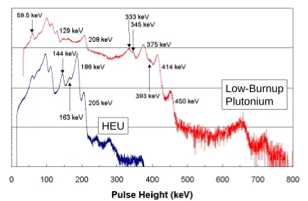
Figure 1.1 Pulse height spectra of highly enriched uranium and low burnup plutonium measured with a CdZnTe detector. ...3 Figure 2.1 The limiting polar angles defined by a detector are a function of the sampled

azimuthal angle. ...12 Figure 2.2 Double differential Compton scattering profiles for an initial gamma-ray

energy of 344keV and a scattering angle of 5°...20 Figure 2.3 Double differential Compton scattering profiles for an initial gamma-ray

energy of 1408keV and a scattering angle of 15°...21 Figure 2.6 Differential Compton scattering cross sections for an initial gamma-ray

energy of 10keV. ...22 Figure 2.7 Differential Compton scattering cross sections for an initial gamma-ray

energy of 344keV. ...23 Figure 2.8 Differential Compton scattering cross sections for an initial gamma-ray

energy of 1408keV. ...23 Figure 2.9 Total Compton cross section comparison between calculated values and

accepted values. ...24 Figure 2.10 Energy Spectra calculated using forcing techniques (blue line) and

MCNP (red line)...26 Figure 2.11 Comparison between Monte Carlo calculation (red line) and experiment

(blue line). The Monte Carlo energy spectrum is calculated using the silicon

detector response function model for a 17x17x1.5 mm silicon detector. ...28 Figure 2.12 Comparison between Monte Carlo calculation (red line) and experiment

(blue line). The Monte Carlo energy spectra are calculated using the appropriate CdZnTe detector response function model. ...28 Figure 3.1 Camera coordinate system for experiment and simulation. ...29 Figure 3.2 Compton camera event diagram...31 Figure 3.3 Single event representation in the form of a rectilinear mapping of

θ and φ (left) and a polar mapping (right). ...32 Figure 3.4 Skymap image coordinate system. ...33 Figure 3.5 Single event representation in the form of a rectilinear mapping of

θ and φ where the xy projection of the event cone contained the origin. ...34 Figure 3.6 Skymap of the calculated response function for a pair of detectors to a

662keV source moved around an event ring. ...36 Figure 3.7 Simulated point source image created by the event circle technique (left) and

(9)

Figure 4.1 A 75Se energy spectrum measured with the 1cm3 CdZnTe detector. ...39

Figure 4.2 Timing calibration spectrum for the preliminary experiment. ...40

Figure 4.3 Preliminary experiment geometry. ...41

Figure 4.4 The coincidence timing spectrum recorded during the preliminary experiment...42

Figure 4.5 Comparison between event circle images produced by simulation (left) and experiment (right). ...42

Figure 4.6 Simple model for the ratio of Compton to random coincident events. ...44

Figure 5.1 Illustration of prototype camera based on two detectors...47

Figure 5.2 Side view (left) and top view (right) of prototype camera. ...48

Figure 5.3 22Na timing calibration spectra for the silicon-CdZnTe (left) and the dual CdZnTe (right) prototype Compton cameras...50

Figure 5.4 CdZnTe detector (ID#315201) energy spectrum of a scene containing a 75Se source and a 137Cs source...51

Figure 5.5 Camera energy sum spectrum (blue line) for a scene containing 75Se and 137Cs. ...52

Figure 5.6 Timing spectrum recorded during an earlier imaging experiment with silicon-CdZnTe prototype camera. ...53

Figure 5.7 Skymap image localizing a 137Cs source in a scene containing both 75Se and 137Cs point sources. ...54

Figure 5.8 Localization of the 75Se source by the 400keV (left) and the 265keV complex (right) in a scene containing both 75Se and 137Cs...54

Figure 5.9 Skymap images created of the 136keV line of 75Se (left) and a background energy window centered at 410keV (right)...55

Figure 5.10 Skymap images of the 265keV complex of 75Se (left) and 662keV line of 137 Cs (right). ...56

Figure 5.11 Comparison of event circle (left) versus EMML (right) image reconstruction for the 662keV line of a 137Cs source...57

Figure 5.12 Comparison of event circle (left) versus EMML (right) image reconstruction for the 662keV line of a 137Cs source...57

Figure 5.13 Sum energy spectrum (blue line) for the dual CdZnTe detector prototype Compton camera. ...59

Figure 5.14 Timing spectrum for the dual CdZnTe prototype camera. ...59

Figure 5.15 Event circle reconstruction of the 137Cs source imaged using the dual CdZnTe prototype camera...60

Figure 5.16 Event circle reconstruction of the 75Se source imaged with the 400keV line (left) and 265keV complex (right)...61

Figure 5.17 Reconstruction of the 137Cs source location (left) and the 75Se source using the 265keV complex...62

Figure 5.18 EMML reconstruction of the 137Cs source location (left) and the 75Se source location (right) using the 265keV complex. This is the same experiment as presented in figures 5.15 and 5.16. ...62

(10)

Figure 6.1 Simulation geometry. ...64

Figure 6.2 Spatial efficiency calculated by FARRAH code (left) and analog code (right). ...65

Figure 6.3 Standard deviation of spatial efficiency calculated by FARRAH code (left) and analog code (right). ...65

Figure 6.4 Simulated images created by event circle method for FARRAH code (left) and analog code (right). ...66

Figure 6.5 Simulation versus experiment for the Si-CdZnTe prototype camera. The experimental data is taken from the camera 9 experiment. The simulation event circle image is created from the 265keV complex of the 75Se source (compare with figure 5.8)...70

Figure 6.6 Simulation versus experiment for the Si-CdZnTe prototype camera. The experimental data is taken from the camera 9 experiment. The simulation event circle image is created from the 662keV line of the 137Cs source (compare with figure 5.7)...71

Figure 6.7 Simulation versus experiment for the dual CdZnTe prototype camera. The experimental data is taken from the camera20_21 experiment. The simulation event circle image is created from the 662keV line from the 137Cs source (compare with figure 5.15)...72

Figure 6.8 Simulation versus experiment for the dual CdZnTe prototype camera. The experimental data is taken from the camera20_21 experiment. The simulation event circle image is created from the 400keV line of the 75Se source (compare with figure 5.16). ...73

Figure 6.9 Magnitude of the low energy cutoff for the front plane detector in the silicon-CdZnTe camera...75

Figure 6.10 Magnitude of the low energy cutoff for the front plane detector in the dual CdZnTe camera...76

Figure 6.11 Camera efficiency over the field of view. ...77

Figure 10.1 Block diagram of preliminary experiment. ...90

Figure 10.2 Photograph of preliminary experiment detector arrangement...93

Figure 10.3 Photograph of electronics for preliminary experiment...94

Figure 10.4 Block diagram of silicon and CdZnTe prototype camera. ...95

Figure 10.5 Silicon detector calibration for converting digitized voltages to energy...98

Figure 10.6 CdZnTe detector (ID#315201) calibration for converting digitized voltages to energy...99

Figure 10.7 Block diagram of dual CdZnTe prototype camera. ...100

(11)

1. Introduction

The goal of spectroscopic imaging is to provide information related to the spatial distribution and identity of radioactive nuclides in a scene. This can be accomplished remotely by the detection of radiation produced from decay of the radioactive isotopes. Imaging systems exist for both gamma-ray and neutron imaging, however our focus will be given to the gamma-ray systems. Specific applications of spectroscopic imaging systems include nondestructive assay of nuclear materials, medical imaging, and gamma-ray imaging for astrophysics. The first two techniques cover energy ranges from about 100keV to 1MeV, while the upper limit for telescopes approaches 30MeV to image high energy cosmic radiation sources.

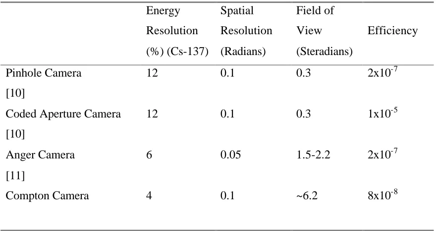
Important parameters for a spectroscopic imaging system are spatial resolution, field of view, detection efficiency, and the energy resolution of the detectors in a system. Spatial resolution defines the ability of a system to resolve two distinct, spatially separated radioactive sources. Field of view defines the solid angle accepted by the system. The amount of time required to examine a given area depends on the system’s field of view and detection efficiency. The ability of a system to distinguish different isotopes is directly related to its energy resolution. A collection of these parameters for some existing gamma-ray imaging systems is contained in table 1.1.

(12)

The motivations for this work are given in the next section followed by a review of gamma-ray imaging systems highlighting limitations of existing designs and the promise of Compton cameras providing a superior match with our requirements. An efficient Monte Carlo code was developed to investigate the image formation processes. Two image reconstruction methods were implemented and compared. To address some of the technical issues, preliminary experimental measurements were made with CdZnTe detectors. Based on these results a prototype camera was fabricated using a two detector system. One of the detectors was mounted on a stage capable of two dimensional motion in order to simulate an array of detectors. Measurements where made using a dual

CdZnTe detector approach and a combination of silicon and CdZnTe detectors. Results of numerical simulations to predict Compton camera performance are reviewed. The implications towards a final system design are discussed.

1.1 Objectives

Safeguarding special nuclear material (SNM) requires knowledge of its location and mass. This can be accomplished using nondestructive assay techniques (NDA)

(13)

HEU

Low-Burnup

Plutonium

Figure 1.1 Pulse height spectra of highly enriched uranium and low burnup plutonium

measured with a CdZnTe detector.

The principal gamma-ray signature for highly enriched uranium is the 186keV line from the 235U isotope and for low burnup plutonium is the 414keV line from 239Pu.

The goal of NDA in this context is to quantify the location and mass of SNM in

(14)

1.2 Literature Review

1.2.1 Gamma-Ray Imaging Systems

Of the multitude of gamma-ray imaging devices that exist, they can be separated into two basic designs: mechanically and electronically collimated systems. Mechanical

collimation is provided by single aperture or an array of holes in a lead shield in front of the detector. Electronic collimation is provided by time coincidence circuitry between spatially separated detectors. High pressure xenon detectors, previously used in high energy physics experiments, form a new class of imaging systems for this energy regime that does not fit into either of the above categories.

A spectroscopic imaging system in its simplest form is the scintillation detector. A NaI(Tl) crystal attached to a photomultiplier, is sensitive to the energy of a detected gamma ray. When coupled to a multichannel analyzer, this class of detectors provides the energy spectrum of gamma rays. By providing a single aperture mechanical collimator made of tungsten or lead, the scintillation detector is now sensitive to the direction of incoming gamma rays. This type of system provides information about one point in a two dimensional spatial image. This point represents the scene integrated over the field of view defined by the collimator. Therefore, the collimator aperture must be scanned over an area to create an image.

If the simple photomultiplier is replaced with a position sensitive photomultiplier, the scene is no longer integrated over the field of view. In order to provide spatial resolution in the image, the collimator aperture is greatly reduced to about 5mm in diameter. This is the principle behind a pinhole camera. As the aperture size is reduced, the spatial

resolution increases at the expense of detection efficiency. A limitation of commercially available systems is that a discriminator window must be set around an isotope’s

(15)

In coded aperture systems the pinhole aperture is replaced with an aperture mask which provides multiple redundant shadows of the scene on the detector crystal [2-5]. If the effect of the mask is deconvoluted from the recorded image via Fourier transforms, the scene is recovered. This technique was originally developed to enhance the signal to noise ratio obtained from a pinhole camera by increasing the detection efficiency (due to the greater open area of the aperture). These systems are especially successful in

recovering the most intense source in a scene with high background. The coded aperture technique does not perform as well as the pinhole camera for imaging spatially extended sources [6]. In addition, image artifacts can be created during the image reconstruction process.

The Anger camera is a large NaI(Tl) crystal coupled to an array of photomultipliers [7]. Mechanical collimation is used to divide the scene into discrete spatial elements on the crystal. The array of photomultiplier tubes provides a position sensitive readout of the crystal. It is the standard imaging device in nuclear medicine. These systems typically have a large field of view. The size and shape of the collimator holes, in large part, determines the system’s spatial resolution and detection efficiency. Three dimensional images of the isotope distribution can be afforded by rotation and translation of the camera around the patient. This provides projection views, which can then be combined by standard tomographic techniques. This technique has been coined by the term Single Emission Computed Tomography (SPECT). The spatial resolution of mechanically collimated systems begins to suffer due to gamma rays over about 250keV penetrating “opaque” portions of the collimator. In general, these systems are not optimized for imaging SNM.

(16)

which gives a trigger signal of the beginning of an event. If incoherent scatter of the gamma ray occurs, the scattered electron produces ionization clusters in the gas. A uniform electric field accelerates the secondary electron clusters produced by the interactions towards a light generating gap over the position sensitive grid. This light generating gap is a region of high electric field where the drifting electrons produce electroluminescence of the gas. The time it takes the light photons to reach the

measurement grid from the beginning of the prompt scintillation gives the depth of the scattered electron track within the chamber. The projection of the photons on the position sensitive grid gives the remaining information needed to reconstruct the three dimensional track of the scattered electrons. Summing the response of all the

photomultipliers, a signal is recorded which is proportional to the energy deposited in each cluster. By measuring the energy and direction of both the scattered gamma and Compton electron, the direction and energy of the incoming gamma ray can be deduced. Note that all the relevant measurements are made within a single detector system. These devices have low noise characteristics making them ideal for low energy measurements below 100keV. Detection efficiency is good due to the high pressure Xenon gas, but they are counting rate limited and errors in reconstruction are introduced by small angle

scattering of the electron before its track is determined.

(17)

the radioactive nuclides in the scene. Image reconstruction can be used to provide image templates identifying the specific locations of each radioisotope. Improvements in CdZnTe detector technology has resulted in the commercial availability of solid state detectors that operate at room temperature with good energy resolution that can be used for this purpose [9]. By relaxing detector cooling requirements, enhanced system portability can be attained. In order to provide competitive detection efficiency with Anger and coded aperture camera systems, arrays of detectors each recording data simultaneously must be used.

Table 1.1 Gamma-ray imaging systems

Energy Resolution (%) (Cs-137)

Spatial Resolution (Radians)

Field of View (Steradians)

Efficiency

Pinhole Camera [10]

12 0.1 0.3 2x10-7

Coded Aperture Camera [10]

12 0.1 0.3 1x10-5

Anger Camera [11]

6 0.05 1.5-2.2 2x10-7

Compton Camera 4 0.1 ~6.2 8x10-8

(18)

those experimentally demonstrated by the silicon-CdZnTe prototype camera (presented in section 6). The Compton camera efficiency is calculated assuming 5x5 array of front plane silicon detectors and 10x10 array of back plane CdZnTe detectors (each the same size as those used in the prototype camera). The time projection chamber is not included in this comparison because data in the literature has not demonstrated actual imaging performance parameters [8].

1.2.2 Compton Camera Systems

A review of existing Compton camera hardware starts with a system developed for astrophysics beginning in 1971 at the Max Plank Institute[12-14]. It matured into the COMPTELpackage implemented on the Compton Gamma-Ray Observatory satellite. The COMPTEL system is comprised of 7 liquid (NE213A) scintillation detectors as the first plane detector array and 14 NaI(Tl) detectors as the second plane detector array. Each of the liquid scintillator cells is 28cm in diameter and 8.5cm deep, instrumented with eight photomultiplier tubes. The individual NaI(Tl) detector crystals are 28.2cm in diameter and are 7.5cm thick, instrumented with seven photomultipliers. The system is designed to image weak, distant sources in the 1-30MeV range. It has an energy resolution of 9% at 1MeV, spatial resolution of 0.02, and a field of view of 1 steradian.

(19)

This same device was improved in 1993 at the University of Michiganby replacing the Anger camera with 16 NaI(Tl) detectors, each 19.1mm in diameter by 50.8mm in length [19-20]. These detectors were arranged in an azimuthal ring behind the Ge array. The system’s spatial resolution was measured at 0.1 radians. Their target application was to measure industrial gamma-ray fields with spatially extended sources composed of more than one isotope. They demonstrated the spectroscopic imaging capability of Compton cameras by imaging a scene containing spatially extended sources of 64Cu (0.511MeV) and 65Zn (1.116MeV). A common thread in all these systems is the use of detectors [NaI(Tl)] with non-optimal energy resolutions for imaging SNM.

The Naval Research Laboratory has designed and tested a system based entirely on high purity Ge detectors for the purpose of characterizing unknowns in radioactive waste containers [21]. These detectors have energy resolutions of 0.3% at 1333keV, which is the best possible for existing detector technology. The associated cryostats used for cooling the detectors makes the system too large to fit with our portable system requirement.

2. Monte Carlo Code Development

Our approach to investigating the Compton camera image formation process and designing a system capable of imaging SNM begins with the development of a Monte Carlo code. Other groups have made Monte Carlo calculations for Compton cameras using little or no variance reduction techniques [22-24]. This is a very inefficient way to simulate Compton camera events from spatially separated detector arrays. Analog Monte Carlo code approaches are inadequate for this research due to the long computation times required.

(20)

response to radiation sources. The principle of pathway sampling via the technique of forcing is used to make each history result in a partial success [25-26]. This technique is based on sampling only the range of a stochastic event that can lead to a success. The weight of the history is adjusted at each such event to reflect the restricted sampling range. Let a particular stochastic event be governed by a normalized probability

distribution function f(x), where x has the range from x_min to x_max. The modified pdf

) ( ˆ _x

f , for forcing x between x₁ and x₂ is obtained from

∫

=

2

1 ) (

) ( )

( ˆ

x

x f x dx x f x

f for xmin ≤ x1 ≤ x≤ x2 ≤ xmax.

The associated weight for forcing x between x₁ and x₂ is

∫

= 2

1 ) (

x

x f x dx

w .

By eliminating ranges of zero probability, no computation time is spent on histories that do not contribute to the result. This technique is only valid when the excluded pathways represent a negligible contribution to the desired result.

The FARRAH code includes effects from Doppler broadening, incoherent scattering functions, peak detector response functions, and multiple Compton scattering. Detailed methodology of the code is outlined in the next section.

2.1 Methodology of FARRAH Code

(21)

defines the convex objects by wire frames and points, instead of using analytical

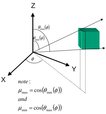
expressions for describing the detectors. This was done to handle orthorhombic shapes of solid state detectors, which we intended to use for this imaging device. The modified pdf for sampling the azimuthal angle is

min max 1 ) ( ˆ φ φ φ − = f ,

where φ_max and φ_min are the limiting azimuthal angles of the detector. The associated weight is π φ φ 2 min max − = w .

After the azimuthal angle is sampled, the modified pdf for sampling the cosine of the polar angle is

( )

φ µ

( )

φ µ µ min max 1 ) ( ˆ − = f ,

where µ_max

( )

φ and µ_min

( )

φ are cosines of the limiting polar angles θ_min and θ_max at azimuthal angle φ, respectively. The associated weight is

( )

2

min max φ µ φ

µ −

=

w .

Note that the azimuthal and polar angles are sampled as independent variables, but the (cosine of the ) limiting polar angles are a function of the sampled azimuthal angle. This is illustrated in figure 2.1. This technique was verified by plotting the intersection

coordinates (determined by the limiting angles) and wire frames of the detectors in 3D for an arbitrary interaction site. In all cases checked, the correct limiting angles were

(22)

Z X Y ( )φ θmin φ ( )φ θmax ( ) ( ) ( ) (θ φ ) µ φ θ µ max min min max cos cos : = = and note

Figure 2.1 The limiting polar angles defined by a detector are a function of the sampled

azimuthal angle.

Once the direction of emission is sampled, a unique path through the detector is defined by this direction and the detector geometry. The gamma ray is forced to have an

interaction somewhere along this path. The modified pdf for forcing an interaction within a distance, D, is

(

)

(

D

)

x x f t t t Σ − − Σ − Σ = exp 1 exp ) ( ˆ _,

where Σ_t is the total macroscopic cross section. The associated weight is

(

D

)

w=1−exp−Σt .

This interaction is forced to be a Compton scattering event by implicit capture. The associated weight for this is

(23)

where Σincoh is the macroscopic incoherent scattering cross section. The scattered gamma ray is then forced in the range of directions defined by the solid angle subtended by one of the detectors in the second plane. This calculation also requires knowledge of limiting azimuthal and polar angles of a detector from a point. First, the azimuthal angle is sampled from a uniform distribution between the calculated limiting angles. The cosine of the polar angle is then sampled from a uniform distribution between the (cosine of the) limiting polar angles. If the scattering medium is a compound, the element which

interacts with the gamma ray is sampled based on the fraction of electrons associated with each element in the compound. Since the pdf governing the incoherent scattering event is the Klein-Nishina formula multiplied by the incoherent scattering function, the weight associated for forcing this interaction to occur is

(

)

(

( )

)

Z Z S f Z

w ( , ) ( , , )

2 )

, , ,

( max min max min α µ α µ

π φ µ φ µ φ φ µ φ α = − − ,

where S(α,µ,Z) is the incoherent scattering function, Z is the atomic number of the scattering element, and f(α,µ) is the Klein-Nishina formula given by [28]

(

)

(

( , ) 1 ( , ) ( , )

)

) ( ) ,

(α µ =K α η3 α µ + µ2 − η2 α µ +ηα µ

f , with

(

µ

)

α µ α η − + = 1 1 1 ) , ( , where 2 0c m E = α .

The parameter α is the initial gamma-ray energy over the rest mass of an electron (511keV). The normalization constant is

(

)

(

2 3

)

(

)

(

3 2

)

(

2

(

)

2

)

2 1 2 8 9 2 2 1 log 2 2 1 ) ( α α α α α α α α α α + + + + + + − − = K .

(24)

around the atom (Doppler broadening). This model is described in detail in section 2.2. The energy deposited in the detector by the scattered electron is simply

s dep E E

E = − ,

where E and E_s are the initial and scattered gamma-ray energies. A detector response function model (section 2.3) is applied to incorporate realistic charge collection

efficiency (reduces the weight) and energy resolution effects (spreads the energy). Now, the scattered gamma ray must escape the first detector. This is accomplished by

weighting the gamma ray by

(

D

)

w=exp −Σ_t ,

where D is the distance out of the detector and Σ_t is the total cross section evaluated at the energy of the scattered gamma ray. The scattered gamma ray is forced to have an energy deposition interaction (either a Compton scatter or a photoelectric absorption) in the second plane detector. If a Compton scatter occurs, the scattered gamma ray is allowed to continue in an analog Monte Carlo fashion until it either escapes this detector or is absorbed by photoelectric absorption. The energy deposited in the second detector is spread by the detector response function and appropriately recorded.

This sequence is repeated from the initial interaction in the first detector to all detectors in the second plane for each history. If there are multiple detectors in the first plane, the next detector is selected and the entire process is repeated.

The issue of multiple Compton scattering in a detector in the first plane before the

scattered gamma ray is emitted towards a second plane detector is also addressed. This is embedded in the previous sequence by forcing other Compton scatters before the gamma ray is allowed to escape the first plane detector. The results of allowing 1, 2, 3, and 4 such scatters are calculated, and can be independently viewed from the final result.

(25)

successful in depositing energy in both of the same detectors as the forced particle, then the forced particle history is killed and the history is repeated.

This scheme creates an efficient code that is capable of predicting the Compton camera response to radiation sources. As with any simulation code, certain assumptions are made to reduce coding complications. These assumptions are explicitly stated and their implications are discussed.

Time is not modeled in the code. Since gamma rays travel at the speed of light, and the camera scale distances are no more than a meter, errors associated with elapsed travel time between detectors are small. As a result of this assumption, chance coincidences that result from high counting rates in each detector plane are not calculated. Also, no mechanism is present to calculate the effect of chance coincidences that result from time correlated gamma-ray emissions from a source. Both of these effects result in an increase in the image background, as compared to simulation.

Only source locations and bare detectors are modeled, none of the surrounding structure around the camera is included in the simulations. These structures could be a source of intermediate scattering and/or attenuation between the source and first detector array or between the first and second detector array. Intermediate scattering would destroy the relationship between the reconstruction cone and the source and result in a reduced signal to noise ratio. Attenuation by either photoelectric absorption or scattering the gamma ray away from the detection arrays would tend to reduce the experimental count rate

compared to that predicted.

(26)

compared to their size and gamma-ray energies below the present range of interest (100keV to 1MeV).

The code does not compute the effects of backscattered gamma rays from the rear plane detector array into the front plane detector array. Since these events could not be discriminated from the forward scatter events, they would create a background in the reconstructed image. The code overestimates the signal to noise ratio for imaging low energy gamma-ray sources since the probability of backscattering increases at low energies.

Effects from gamma rays scattering between multiple elements in a detector array before being detected in the second array are not considered. Only two detectors are simulated at a time in the code, while the rest of the detectors in the arrays are ignored. If a gamma ray deposited energy in two or more detectors in one array and in one or more detectors in the other array, the relationship between the reconstruction cone and the source would be lost. Such an event would contribute to the background in the reconstructed image. These events would represent only a small fraction of detected events since it requires at least three energy deposition events in three different detectors.

2.2 Doppler Broadening Model

(27)

no energy is absorbed by the atoms during the scattering process and the atoms are free, i.e. no molecular effects. This technique was used in the EGS4 Monte Carlo code for including the Doppler broadening of a Compton scattered photon’s energy [29-30]. These routines were verified and validated by comparisons of the double differential, differential, and total incoherent scattering cross sections to values published in the literature.

Once a Compton event is indicated in the simulation, the parameters governing the interaction are initial gamma-ray energy and atomic number of the atom involved in the scattering process. If the medium in which a Compton event occurs is a compound, the specific element the gamma ray interacts with is sampled based on the fraction of

electrons associated with each element in the compound. The code provides output of the final scattered gamma-ray energy, and cosine of the polar scattering angle. Since only unpolarized photons are considered, the azimuthal scattering angle is sampled uniformly over the range [0,2π].

The cosine of scattering polar angle, µ, is calculated using the Kahn rejection technique which samples from the Klein-Nishina formula exactly [31]. Another rejection technique is then used to account for the incoherent scattering function, S(x(µ,αi),Z), where the scattered polar angle is retained with a probability of

1 ) ), , 1 ( (

) ), , ( (

≤

− Z

x S

Z x

S

i i α α µ

.

A description of this technique is contained in the appendix, section 10.1. The incoherent scattering function, for 1≤Z ≤100, is tabulated as a function of the momentum transfer variable, x(µ,α_i), in units of inverse Angstroms,

µ α

α

µ, )=29.143 1−

( _i _i

x ,

(28)

incoherent scattering function between the tabulated points, except between the first two points where linear interpolation is used.

Once the scattering polar angle is determined, the scattered photon’s energy is calculated using shellwise Compton profiles as probability distribution functions. The Compton profiles are tabulated as a function of the projection of the electron pre-collision momentum on the momentum transfer vector of the gamma ray. This projected momentum is described by

µ µ s i s i s i s i z E E E E c m E E E E p 2 ) 1 ( 137 2 2 2 0 − + − − − − = ,

where p_z is the momentum in atomic units of 2 h

0e

m (the average electron momentum in the ground state of hydrogen), and Es is the scattered gamma-ray energy [33]. The Compton profiles, Jk(pz,Z), for the elements 1≤Z ≤102 have been calculated and are symmetric about px =0 [34]. Note that these profiles are related to the incoherent scattering function by

∑∫

−∞ = k p z z k i k dp Z p J Z

S(µ,α , ) ,max ( , ) ,

where the subscript k refers to the particular electron subshell and pk,maxis obtained from

the equation for p_z by substituting b k i s E E E = − ( b

k

E is the binding energy of the electrons in the kth shell).

(29)

where ξ is a random number from a uniform distribution contained on [0,1]. These integrals are calculated numerically assuming linear interpolation between the points (the denominator is precomputed). Once the value of p_z is sampled, the scattered gamma-ray energy is the only unknown in the momentum equation. The equation is quadratic in E_s,

0

2 + + =

C BE

AE_s _s ,

where 2 2 2 0 2 2 2 0 2 2 0 2 137 2 ) 1 ( 2 137 2 1 ) 1 ( 2 ) 1 ( 137 i i z i i i z i i z E E p C E c m E E p B c m E c m E p A −       = + − +       − = − − −     − −       = µ µ µ µ .

Of the two possible roots, one is randomly selected. If the scattered energy is greater than the maximum possible value determined by E_s,max = E_i −E_b (Eb is the binding energy of an electron in the kth subshell [35]), or is negative, the sample is rejected and the process is repeated. Occasionally imaginary roots are possible due to numerical fluctuations. When this occurs, the sample is rejected and the process is repeated.

2.2.1 Verification of Doppler Broadening Model

(30)

Figure 2.2 Double differential Compton scattering profiles for an initial gamma-ray energy of 344keV and a scattering angle of 5°. A comparison of simulation results using the Monte Carlo model (histogram) and theoretical calculations (red line) is presented for

carbon (left) and lead (right).

Figure 2.3 Double differential Compton scattering profiles for an initial gamma-ray

energy of 344keV and a scattering angle of 15°. A comparison of simulation results using the Monte Carlo model (histogram) and theoretical calculations (red line) is

(31)

Figure 2.4 Double differential Compton scattering profiles for an initial gamma-ray energy of 1408keV and a scattering angle of 5°. A comparison of simulation results using the Monte Carlo model (histogram) and theoretical calculations (red line) is

presented for carbon (left) and lead (right).

Figure 2.5 Double differential Compton scattering profiles for an initial gamma-ray

energy of 1408keV and a scattering angle of 15°. A comparison of simulation results using the Monte Carlo model (histogram) and theoretical calculations (red line) is

presented for carbon (left) and lead (right).

Apparent in all of these figures is a shift in scattered photon energy between the

(32)

to the case when the determinate of the solution the momentum equation is zero). The derivation of the momentum equation is based on energy-momentum conservation assuming free particle kinematics. Therefore, the energy peak from these routines will always be at the free electron scatter energy. The relativistic impulse approximation solutions do not contain any assumptions regarding the energy value of the peak.

The single differential Compton scattering cross section was calculated by numerical integration of the double differential cross section over the scattered photon energy. The double differential cross section was discretized into 1000 energy bins and 360 polar angle bins (the azimuthal angle was not discretized) for 107 histories. The energy range

covered was _s _i

i i

E E

E

1 . 1 2

1 01 . 0

≤ ≤

+ α , and polar angle range was

[

0,2π

]

. The integral was properly normalized and compared to a direct calculation of the Klein-Nishina formula multiplied by the incoherent scattering function. These comparisons are presented in figures 2.6-2.8, for carbon and lead at initial photon energies of 10, 344, and 1408keV.

Figure 2.6 DifferentialCompton scattering cross sections for an initial gamma-ray

(33)

Figure 2.7 Differential Compton scattering cross sections for an initial gamma-ray energy of 344keV. A comparison of simulation using the Monte Carlo model (histogram) and direct calculation (red line) is presented for carbon (left) and lead (right).

Figure 2.8 Differential Compton scattering cross sections for an initial gamma-ray

(34)

subroutines are capable of calculations below 10keV, although runtime may become excessive due to reduced efficiency of the incoherent scattering function rejection technique.

Figure 2.9 Total Compton cross section comparison between calculated values and

accepted values.

2.3 Detector Response Function Models

(35)

function models are used in conjunction with Monte Carlo simulations on a single event basis.

For coplanar grid CdZnTe detectors, the line shape about E₀can be represented by the combination of a Gaussian and two exponential tails for low and high energy tailing about the peak [37],

(

( ) ( )

)

) ( )

(E G E f Tail E Tail E

Peak = + _hi + _lo ,

where      ₋ −

= ₂0 2

2 ) ( exp 2 1 ) ( σ σ π E E E G ,

(

)

(

)

(

)

(

)

       + − −         +                 ₋ − + − = hi hi hi hi hi hi hi E E E E E E E erf E Tail µ α µ σ α σ µ σ α 0 0 2 0 0 0 2 exp 2 2 1 2 1 ) ( ,

(

)

(

)

(

)

(

)

       + − −         +                 ₋ − + − = lo lo lo lo lo lo lo E E E E E E E erf E Tail µ α µ σ α σ µ σ α 0 0 2 0 0 0 2 exp 2 2 1 2 1 ) ( .

The six parameters needed to describe the line shape are f , σ , αhi, αlo, µhi, and µlo. They are determined from experimental spectra by using a nonlinear least squares fitting algorithm. Experimental spectra were measured for 241Am, 133Ba, 57Co, and 137Cs. These experiments provided photopeak calibration energies of 60, 81, 122, and 662 keV,

respectively. The full energy efficiency is determined by dividing the measured photopeak area by a photopeak area determined from a Monte Carlo calculation.

(36)

not statistically significant, the charge collection efficiency is determined by a comparison of the Compton edge magnitude for both calculation and experiment. Experimental spectra were measured for 22Na, 137Cs, and 54Mn. These experiments provided clean Compton edges at 341, 477, and 639 keV.

In order to validate the Monte Carlo calculations using forcing techniques, similar runs were made with MCNP (version 4B) using no variance reduction [38]. Each simulation consisted of a bare detector and a 662 keV monoenergetic source separated by 1 cm. Comparisons of the calculated energy spectra are made for both CdZnTe and silicon detectors in figure 2.10.

Figure 2.10 Energy Spectra calculated using forcing techniques (blue line) and MCNP

(red line). The figure on the left is for a 15x15x8mm CdZnTe detector and on the right is a for 17x17x1.5mm silicon detector. The spectra are not normalized.

After the energy spectra are calculated using MCNP, they are convolved with a Gaussian distribution. The additional structure seen in the Compton edge of the MCNP spectra is related to the fact that MCNP does not use the Doppler broadening method for

calculation of the Compton scattered photon energy. Doppler broadening, by its very nature, provides further smoothing through the Compton edge.

(37)

collection efficiency is modeled as a piecewise linear function of energy bounded between zero and one.

Table 2.1 Detector response function parameters

Energy Spread Parameters Charge Collection Efficiency, ε(keV)

Intrinsic Silicon Detector (17x17x1.5 mm)

Noise, σ =13keV

80 . 0 ) 639 ( 85 . 0 ) 477 ( 00 . 1 ) 341 ( = = = ε ε ε

Coplanar Grid CdZnTe Detector ID# I315201 (15x15x8 mm) . 0 . 0 . 64 . 90 38 . 2 75 . 0 = = = = = = hi lo hi lo f µ µ α α

σ (662) 0.31

32 . 0 ) 122 ( = = ε ε

Cylindrical Coplanar Grid CdZnTe Detector

ID# C26-05

(10 mm diameter by 5 mm thick) . 1 . 1 . 45 . 55 20 . 3 11 . 0 = = = = = = hi lo hi lo f µ µ α α

σ (662) 0.5

5 . 0 ) 551 ( = = ε ε

The 137Cs experiments, used to calibrate the response function models are presented in figure 2.11 and 2.12. The Monte Carlo simulations consisted of a bare detector and a 662keV monoenergetic point source in same geometry as the experiment. The effect produced from multiple Compton scattering in the detector was included in the

(38)

Figure 2.11 Comparison between Monte Carlo calculation (red line) and experiment (blue line). The Monte Carlo energy spectrum is calculated using the silicon detector

response function model for a 17x17x1.5 mm silicon detector.

Figure 2.12 Comparison between Monte Carlo calculation (red line) and experiment

(blue line). The Monte Carlo energy spectra are calculated using the appropriate CdZnTe detector response function model. The figure on the left is for a 10mm diameter by 5mm

(39)

Although the peak areas match, the CdZnTe simulations underestimate the magnitude of the Compton continuum. The silicon detector energy spectrum also exhibits structure below 400keV that the simulation does not produce. Both of these features may be explained by incomplete charge collection. If a small fraction of deposited charge undergoes recombination, is trapped by crystal imperfections, or escapes from the crystal a background would be produced in the spectra consistent with these observations. These discrepancies are not important since only the peak response function model is needed.

3. Image Reconstruction Techniques

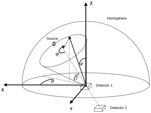
The coordinate system used with the camera is illustrated in figure 3.1. The origin is located at the center of the front face of the front plane detector array.

Z X Y

Y

θ

φ

Source

Com pton Cam_era

Front Plane Array Second

Plane Array

Figure 3.1 Camera coordinate system for experiment and simulation.

(40)

specific gamma-ray emission energy characteristic of the desired radioisotope to be imaged. In addition, the cone half angle is required to be between zero and ninety degrees. One further imposed limitation requires the energy deposited in the second plane detector be less the lower limit of the energy window. This effectively removes events where a noise pulse is recorded in the first plane detector and a photoelectric event occurs in the second plane detector.

Image reconstruction of source positions from Compton camera data (experiment or simulation) is done by one of two techniques: event circle or Expectation Maximum-Maximum Likelihood (EMML). Both produce two dimensional images represented by the spherical coordinatesθand φ. The image space uses a colormap that is proportional to the probability of the source being located at that particular position.

3.1 Event Circle Method

Event circles are the fundamental representation of Compton camera data. It is the most direct technique of mapping the camera data into image space. The image space is created by projecting a cone (reconstructed from the locations and energies deposited in the detectors) onto a hemispherical surface for each recorded event. The hemisphere is centered at the coordinate system origin. Its radius must be greater than the distance between any source within the field of view and the camera. The cone axis lies along the direction connecting the centers of the two detector elements. The cone apex is located at the center of the first detector element. The Compton energy angle relationship is used to determine the cone half angle, γ , from the energy deposited in each detector,

( )

_

  

  

− +

+ =

2 2

1 2 0

1 1

1 cos

dep dep

dep E E E

c m

γ ,

where γ∈[0,π 2]. This couples the camera spatial resolution to the energy resolution of the detectors. Since only unpolarized gamma rays are considered, the azimuthal angle,

(41)

Detector 1 Source

γ

Detector 2

ϕ

Hemisphere

X

Y

Z

φ

θ

Figure 3.2 Compton camera event diagram. For a single event, a reconstruction cone is

created by sampling many rays along the cone’s surface. The intersection of a ray with the hemisphere is plotted in image space represented by θand φ. In general, note that

the hemisphere is centered on the front face of the first detector array. The intersection of the rays along the surface of the reconstruction cone and the hemisphere are computed. Each intersection point is represented in spherical

coordinates, θand φ, and mapped onto the image space. The locus of intersection points for a single Compton scattering event creates a circle when viewed along the cone axis. Each event is processed in this manner and added to the existing image space. After many events are recorded, the location of the source is reinforced such that it stands out over the background.

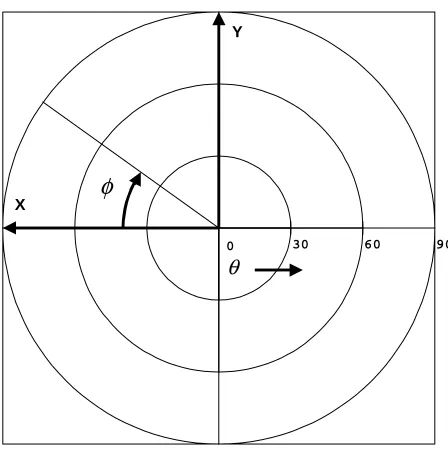
3.2 Image Space Maps

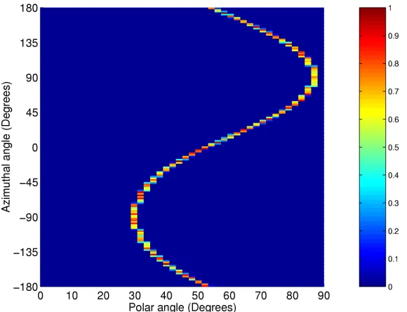
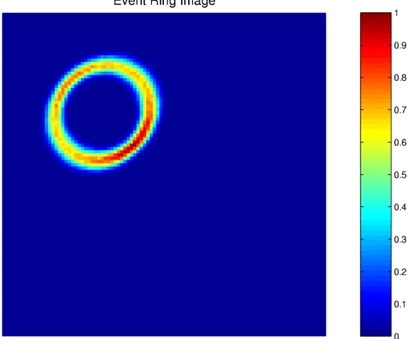
Two types of image representation have been used. The spherical coordinates, θand φ, have been plotted using a rectilinear grid and a polar grid. Earlier images from

(42)

intersections produced by a single event cone with the hemisphere is presented in figure 3.3 for both types of images.

Figure 3.3 Single event representation in the form of a rectilinear mapping of θ and φ

(left) and a polar mapping (right). The event cone had a half angle of 25°, the center of the front plane detector was at (0,0,-0.07 cm), and center of the back plane detector was

at (-7 cm,-7 cm,-9.5 cm).

Illustrated in figure 3.4 is the skymap coordinate system which represents the field of view from the perspective of the camera. Although each image in figure 3.3 contains the same information, the skymap (polar grid) is a more intuitive representation. This type of representation of spherical coordinates in a flat plane is known to cartographers as a polar azimuthal equidistant projection [39]. Distances measured on the skymap are equal to distances measured on the surface of the hemisphere. This feature removes the need for pixel normalization, since each pixel on the map represents the same area on the

(43)

30 60 0 90 θ φ X Y

Figure 3.4 Skymap image coordinate system. The field of view is represented from the

perspective of the camera which is centered at the origin. Since the field of view is only the hemisphere in front of the camera, the area of the corners outside the θ =90circle do

not contain any image information.

Each pixel in the rectilinear mapping requires a normalization which corrects for the differences in area between the map and the hemisphere. This normalization is

(

1

)

, cos cos sin 1 1 1 1 + − ∆ = =

∫ ∫

+ + + + i i sphere i i i i i i i i d d d d A A θ θ θ φ θ θ φ θ φ φ θ θ φ φ θ θ φ θ .

In general for these maps, the pixel dimensions are two degrees square. Note the azimuthal axis is compressed compared to the polar axis. The variation in intensity around the pattern for a single event is due to both quantization of the spherical angles and the coordinate system to which they are referenced. Sinusoidal patterns can be produced in the rectilinear mapping if a projection of the intersection points on the xy plane contains the origin. An example is illustrated in figure 3.5. Sources located near the z axis also present a problem for the rectilinear mapping. If the polar angle

(44)

Figure 3.5 Single event representation in the form of a rectilinear mapping of θ and φ where the xy projection of the event cone contained the origin. The event cone had a half

angle of 57°, the center of the front plane detector was at (0,0,0 cm), and center of the back plane detector was at (0,-3 cm,-6 cm).

3.3 Expectation Maximum-Maximum Likelihood Method

Image reconstruction is also performed by the expectation maximum-maximum

likelihood technique [40]. The EMML method casts the image reconstruction problem in terms of a conditional probability function,

( )

(

)

∏∏

−

=

i

j i j j i

d j i j

f p d

f p f

d g

i exp ! )

|

( ,

(45)

A recorded event is binned into the ordered event vector, di, parameterized by the spherical coordinates of the cone axis (αandδ ) and half angle (γ ). A row in the probability function array, pi_j, is constructed for each discrete element in the event vector. The ith row in the probability function array is the normalized event circle image (the response function) created by an event with parameters α, δ , and γ . These images are represented by an ordered vector (denoted by subscript j) in terms of the spherical coordinates in the image space (θ and φ). The EMML algorithm that maximizes the likelihood function is

j k j k j k j a b f f +1 = , where

∑

= i k j i j i j i k j f p p d b , and

∑

= i i j j p a .

The integer k is the iteration index. An initial estimate of the image is provided such that 0

0 _>

j

f for all j.

The estimate of the image is updated until the global error criterion,

01 . 0 1 1 ≤         ₋ =

∑

₊ + j k j k j k j f f f error , is met.

(46)

A row in the probability function array is essentially the response function for a specific detector pair and cone half angle. For computational efficiency, it is computed assuming point detectors which produce event rings of approximately one pixel in width (see the skymap image in figure 3.3). An actual detector pair response to a source was calculated using Monte Carlo and is presented in figure 3.6.

Figure 3.6 Skymap of the calculated response function for a pair of detectors to a

662keV source moved around an event ring. The nominal scattering angle is 25°. The front plane detector was composed of silicon with a pitch of 1.7 cm and height of 0.15 cm. The second plane detector was CdZnTe with a pitch of 1.5 cm and height of 0.8 cm.

The detector centers where located at the same positions as in figure 3.3.

(47)

3.4 Technique Comparison Using Simulation

A comparison of image reconstruction methods demonstrates the advantage of the EMML technique over the event circle method, shown in figure 3.7.

Figure 3.7 Simulated point source image created by the event circle technique (left) and

by the EMML technique (right).

The camera geometry is the same as shown in figure 6.1. The event circle method

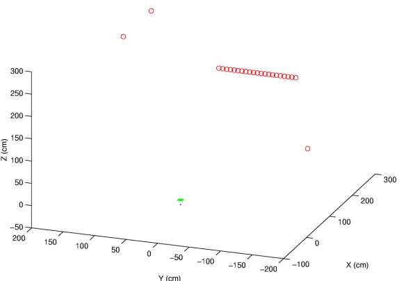
produces a large background associated with the point source. The effect of this becomes evident in a simulation of the same camera with multiple sources contained in the scene. The scene, illustrated in figure 3.8, contains three point sources and a line source

(48)

Figure 3.8 Multiple source simulation geometry. The camera is composed of an array of front plane detectors (green) and a single back plane detector (blue). The red circles

indicate the locations of the 137Cs sources.

The reconstructed images can be seen in figure 3.9, for the event circle and EMML methods, respectively.

Figure 3.9 Multiple source simulation images reconstructed by event circle method (left)

and EMML technique (right).

(49)

EMML image recovers this, while the event circle image is dominated by the line source because of the multiple reinforcement caused by its large point spread function.

4. Preliminary Compton Camera Experiment

4.1 Description

A preliminary experiment was set up to test the detectors, electronics, and limiting technical issues. This simple experiment used a two detector system to locate a 1.2mCi

75

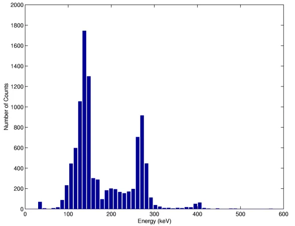
Se source. In order to provide source localization using the Compton camera technique, one detector had to be physically moved in relation to the other detector. Two CdZnTe coplanar grid detectors were setup with timing electronics and a digital data acquisition system. A block diagram of the experimental setup and electronics settings, along with photographs of the system, is presented in the appendix, section 10.2. The first detector was 10x10x5mm in size and has an energy resolution of 4% at 0.662MeV. The second detector was 10x10x10mm in size and has an energy resolution of 2.5% at 0.662MeV. A measured energy spectrum of 75Se decay is presented in figure 4.1.

Figure 4.1 A 75Se energy spectrum measured with the 1cm3 CdZnTe detector. Three

(50)

The timing electronics were calibrated using a 22Na source, which decays with a positron emission component. 22Na is a convenient calibration source due to the two correlated 0.511MeV gamma rays produced by the annihilation of the positron. The calibration timing spectrum is presented in figure 4.2. The peak in this spectrum corresponds to zero time difference between energy deposition events in each detector. A timing window of 2µs wide, centered on this peak, was used for the experiment. Energies deposited in each detector were digitized only when the time difference between the corresponding timing pulses occurred within this window.

In addition to the 0.511MeV annihilation radiation, a 1.275MeV gamma ray is also present from 22Na decay. The spectral peaks at these two energies provided a two point, linear energy calibration for each detector.

Figure 4.2 Timing calibration spectrum for the preliminary experiment. The

annihilation radiation produced during decay of 22Na provided two correlated gamma rays at the same time. The full width half maximum is 800ns.

(51)

counting rates in each detector. Three measurements were made to provide image data, where the first detector was raised in 2cm increments. The geometry is illustrated in figure 4.3. Ten thousand coincident events were recorded at each position.

Figure 4.3 Preliminary experiment geometry. The red circle represents the source, each

of the first plane detector locations are in green, and the second plane detector is blue.

4.2 Results

(52)

Figure 4.4 The coincidence timing spectrum recorded during the preliminary experiment.

The peak to backgound ratio in the timing spectrum is nearly unity.

The experiment was simulated with the FARRAH code assuming a monoenergetic 400keV point source. A comparison the images produced by the event circle method for the simulation and the experiment is contained in figure 4.5.

Figure 4.5 Comparison between event circle images produced by simulation (left) and

(53)

The experiment image was produced using only the detected events whose energy sum was within 4% of 400keV. The discrepancy in the source location is attributed to the incomplete knowledge of the source location. The source was contained in a 7cm long lead cylinder with open ends. The exact location of the source with respect to the end of the cylinder was not known and a best guess was made for the simulation.

4.3 Discussion

Although the preliminary results were encouraging, the experiment brought forth some technical issues that needed to be addressed before building a prototype camera: random coincidences and detector noise.

The number of random coincidences is proportional to the product of the count rates in each detector and the width of the coincidence timing window. In the preliminary experiment, the number of random coincidences where reduced by placing shielding between the source and second detector. This was easy in our controlled experiment, but may be more difficult for an unknown scene with high fluxes. It is generally an

(54)

2 2 1 sep t inc d d t S Random Compton           ∆ = µ µ sep

d

1st Detector Plane 2nd Detector Plane

d

Source

Figure 4.6 Simple model for the ratio of Compton to random coincident events. The

variables represented are: source activity, S, width of the coincidence timing window, ∆t, incoherent scattering cross section, µ_inc, total cross section, µ_t, and the distances, d and

sep d .

This simple model predicts that the ratio of Compton to random coincidence events increases as the square of the distance of the source to the camera. Therefore, the signal to noise ratio of the image improves as the camera is moved away from the source distribution to be imaged.

A further increase in the ratio of Compton to random coincidence events can be achieved by reducing the width of the coincidence timing window. As noted in the preliminary experiment, the width of the window was set to 2µs to capture the timing peak produced during calibration with the 22Na source. The required window width did not agree with the apparent 100ns pulse rise time of the CdZnTe detectors. This is due to the physics of coplanar grid charge collection [42].

The spectroscopy signal from the coplanar detector is derived from differencing the signals induced on the interdigital collecting and noncollecting grids. In CdZnTe