Finding Spatio-Temporal Patterns in Climate Data Using Clustering
1
Mohd. Noor Md. Sap,
2A. Majid Awan
Faculty of Computer Sci. & Information Systems, University Technology Malaysia
Skudai 81310, Johor, Malaysia
1
[email protected],
2[email protected]
Abstract
This paper presents a method for unsupervised partitioning of data for finding spatio-temporal patterns in climate data using kernel methods which offer strength to deal with complex data non-linearly separable in input space. This work gets inspiration from the notion that a non-linear data transformation into some high dimensional feature space increases the possibility of linear separability of the patterns in the transformed space. Therefore, it simplifies exploration of the associated structure in the data. Kernel methods implicitly perform a non-linear mapping of the input data into a high dimensional feature space by replacing the inner products with an appropriate positive definite function. In this paper we present a robust weighted kernel k-means algorithm incorporating spatial constraints for clustering climate data. The proposed algorithm can effectively handle noise, outliers and auto-correlation in the spatial data, for effective and efficient data analysis by exploring patterns and structures in the data.
1. Introduction
Data clustering, a class of unsupervised learning algorithms, is an important and applications-oriented branch of machine learning. Its goal is to estimate the structure or density of a set of data without a training signal. It has a wide range of general and scientific applications such as data compression, unsupervised classification, image segmentation, anomaly detection, etc. There are many approaches to data clustering that vary in their complexity and effectiveness, due to the wide number of applications that these algorithms have. While there has been a large amount of research into the task of clustering, currently popular clustering methods often fail to find high-quality clusters.
A number of kernel-based learning methods have been proposed in recent years [3, 7, 8, 9, 15, 16, 21]. However, much research effort is being put up for improving these techniques and in applying these techniques to various application domains. Generally speaking, kernel function implicitly defines a non-linear transformation that maps the data from their original space to a high dimensional space where the data are expected to be more separable. Consequently, the kernel methods may achieve better performance by working in the new space. While powerful kernel methods have been proposed for supervised classification and regression problems, the development of effective kernel method for clustering, aside from a few tentative solutions [4, 9, 17], needs further investigation.
Finding good quality clusters in spatial data (e.g, temperature, precipitation, pressure, etc) is more challenging because of its peculiar characteristics such as auto-correlation, non-linear separability, outliers, noise, high-dimensionality, and when the data has clusters of widely differing shapes and sizes [11, 18, 22]. With this in view, the intention of this paper is, firstly, to analyze selective kernel-based clustering techniques in order to identify how further improvement can be made especially for spatial data clustering. Finally, we present a weighted kernel k-means clustering algorithm incorporating spatial constraints bearing spatial neighborhood information in order to handle spatial auto-correlation and noise in the spatial data.
handling noise, outliers and auto-correlation in the spatial data. In order to speed up computations, use of triangular inequality is described in section 6. Finally in section 8, brief discussion and conclusion are given.
2. Application area and methods
This work is focusing on clustering spatial data, e.g. for finding patterns in rainfall, temperature, pressure data so that their impact on other objects like vegetation etc could be explored. A very simplified view of the problem domain might look like as shown in Figure 1. The data for the problem domain might consist of a sequence of snapshots of the earth areas taken at various points in time, as shown in the figure. Each snapshot might consist of measurement values for a number of variables e.g., temperature, pressure, precipitation, etc. All attribute data within a snapshot is represented using spatial frameworks, i.e., a partitioning of the study region into a set of mutually disjoint divisions which collectively cover the entire study region. This way we would be dealing with spatial time series data.
Temperature Precipitation
…
Pressure
Temperature Precipitation
…
Pressure
Longitude
Latitude
Time
grid cell zone
. .
.
Fig. 1. A simplified view of the problem domain
Clustering, often better known as spatial zone formation in this context, segments land into smaller pieces that are relatively homogeneous in some sense. While these zones can be specified directly by researchers, clustering provides a general data mining approach for automatically creating zones. Thus, our basic approach is to treat the zone creation problem as a cluster analysis problem. Cluster analysis groups objects (grid cells) so that the objects in a group are similar to one another and different from the objects in other groups. A goal of the work is to use clustering to divide areas of the land into disjoint regions in an automatic, but meaningful way that enables us to identify regions of the land whose constituent points have similar short-term and long-term characteristics. Given relatively uniform clusters we can then identify how various phenomena or parameters, such as precipitation, influence the climate and oil-palm produce (for example) of different areas.
The spatial and temporal nature of our target data poses a number of challenges. For instance, such type of earth science data is noisy. In addition, such data displays autocorrelation (i.e., measured values that are close in time and space tend to be highly correlated, or similar), high dimensionality (for example, if we consider monthly precipitation values at 1000 spatial points for 12 years, then each time series would be 144 dimensional vector), clusters of non-convex shapes, outliers.
If we apply a clustering algorithm to cluster time series associated with points on the land, we obtain clusters that represent land regions with relatively homogeneous behavior. The centroids of these clusters are time series that summarize the behavior of these land areas, and can be represented as indices. Consequently, clustering is an initial and key step in using data mining for the discovery of indices. Afterwards, the correlation between the clusters we have found can be analyzed.
Next, the influence of potential indices on land points can be evaluated. Specifically, we are interested in using a time series (cluster centroid, or otherwise) as indices if it can be used to explain the behavior of a well-defined region of the land, especially with respect to oil palm yield. One way of evaluating impact of indices on the land is to compute the correlation of each cluster centroid with each land point, where the behavior of a land point is described by a time series which captures the time dependent behavior of some variable (e.g., precipitation, temperature, pressure, humidity, oil-palm yield) associated with the land point. In this fashion, we can determine, for each land point, the cluster centroid with which it is most highly correlated.
3. Kernel-based methods
feature space will undoubtedly lead to an exponential increase of computational time, i.e., so-called curse of dimensionality. Fortunately, adopting kernel functions to substitute an inner product in the original space, which exactly corresponds to mapping the space into higher-dimensional feature space, is a favorable option. Therefore, the inner product form leads us to applying the kernel methods to cluster complex data [9, 15].
3.1 Support vector machines and kernel-based methods
Support vector machines (SVM), having its roots in machine learning theory, utilize optimization tools that seek to identify a linear optimal separating hyperplane to discriminate any two classes of interest [19, 20]. When the classes are linearly separable, the linear SVM performs adequately.
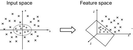
There are instances where a linear hyperplane cannot separate classes without misclassification, an instance relevant to our problem domain. However, those classes can be separated by a nonlinear separating hyperplane. In this case, data may be mapped to a higher dimensional space with a nonlinear transformation function. In the higher dimensional space, data are spread out, and a linear separating hyperplane may be found. This concept is based on Cover’s theorem on the separability of patterns. According to Cover’s theorem on the separability of patterns, an input space made up of nonlinearly separable patterns may be transformed into a feature space where the patterns are linearly separable with high probability, provided the transformation is nonlinear and the dimensionality of the feature space is high enough. Figure 2 illustrates that two classes in the input space may not be separated by a linear separating hyperplane, a common property of spatial data, e.g. rainfall patterns in a green mountain area might not be linearly separable from those in the surrounding plain area. However, when the two classes are mapped by a nonlinear transformation function, a linear separating hyperplane can be found in the higher dimensional feature space.
Let a nonlinear transformation function φ maps the data into a higher dimensional space. Suppose there exists a function K, called a kernel function, such that,
) ( ) ( ) ,
(xi xj xi xj
K =φ ⋅φ
A kernel function is substituted for the dot product of the transformed vectors, and the explicit form of the transformation function φ is not necessarily known. In this way, kernels allow large non-linear feature spaces to be explored while avoiding curse of dimensionality. Further, the use of the kernel function is less
computationally intensive. The formulation of the kernel function from the dot product is a special case of Mercer’s theorem [16].
Fig. 2. Mapping nonlinear data to a higher dimensional feature space where a linear separating hyperplane can be found, eg, via the nonlinear map
(
[ ] [ ]
[ ][ ]
1 2)
2 2 2 1 3 2
1, , ) , , 2 (
)
(x = z z z = x x x x
Φ
Examples of some well-known kernel functions are given below:
• Polynomial: d
j i j
i x x x
x
K( , )=< , >
• Radial Basis Function (RBF):
) 2 / exp(
) ,
( 2 σ2
j i j
i x x x
x
K = − −
• Sigmoid: K(xi,xj)=tanh(α <xi,xj >+β)
4. K-means and kernel methods for
clustering
Clustering has received a significant amount of renewed attention with the advent of nonlinear clustering methods based on kernels as it provides a common means of identifying structure in complex data [2, 4, 9, 15]. Before discussing two kernel-based algorithms [2, 4] here, the popular k-means algorithm is described in the next subsection, which is used as predominant strategy for final partitioning of the data.
4.1 K-means
First we briefly review k-means [12] which is a classical algorithm for clustering. We first fix the notation: let X = { xi }i=1, . . .,n be a data set with xi∈ RN
. We call codebook the set W = { wj }j=1, ., ., .,k with wj∈
RN and k << n. The Voronoi set (Vj ) of the codevector
wj is the set of all vectors in X for which wj is the
nearest vector, i.e.
} min
{
,...,
1 k i j
j i
j x X j arg x w
V = ∈ = −
=
For a fixed training set X the quantization error E(W ) associated to the Voronoi tessellation induced by the codebook W can be written as
2
1
)
(
∑ ∑
= ∈ −
= k
j x V
j i
j i
w x W
E (1)
K-means is an iterative method for minimizing the quantization error E(W) by repeatedly moving all codevectors to the arithmetic mean of their Voronoi sets. In the case of finite data set X and Euclidean distance, the centroid condition reduces to
∑
∈= j iV
x i j
j x
V
w 1 (2)
where |Vj| denotes the cardinality of Vj . Therefore,
k-means is guaranteed to find a local minimum for the quantization error. However, the k-means does not have mechanism to deal with issues such as:
• Outliers; one of the drawbacks of k-means is lack of robustness with respect to outliers, this problem can be easily observed by looking at the effect of outliers in the computation of the mean in eq. (2).
• non-linear separability of data in input space,
• auto-correlation in spatial data,
• noise, and high dimensionality of data.
4.2 One class SVM
Support vector clustering (SVC) [2], also called one-class SVM, is an unsupervised kernel method based on support vector description of a data set consisting of positive examples only. In SVC, data points are mapped from data space to a high dimensional feature space using a Gaussian kernel. In feature space, SVC computes the smallest sphere that encloses the image of the input data. This sphere is mapped back to data space, where it forms a set of contours, which enclose the data points. These contours are interpreted as cluster boundaries.
The clustering level can be controlled by changes in the width parameter of the Gaussian kernel (σ). The SVC algorithm can also deal with outliers by employing a soft margin constant that allows the sphere in feature space not to enclose all points.
Since SVC is using a transformation to an infinite dimension space, it can handle clusters of practically any shape, form or location in space. This is probably its most important advantage. However, the algorithm has the following drawbacks:
• One problem with the algorithm is its extreme dependence on σ. Finding the right value of σ is time-consuming and very delicate.
• Another disadvantage of the algorithm is its complexity. The separation of the sphere to different clusters and determining the adjacency matrix is extremely complicated.
• As the number of dimensions increases, the running time of the algorithm grows dramatically. For a large number of attributes, it is practically not feasible to use this algorithm.
4.3 Mercer kernel k-means
In [4], F. Camastra and A. Verri report on extending the SVC algorithm. The kernel k-means algorithm [4] uses k-means like strategy in the feature space using one class support vector machine. The algorithm can find more than one clusters. Although the algorithm [4] gives nice results and can handle outliers but it has some drawbacks:
• The convergence of this procedure is not
guaranteed and is an open problem. The algorithm does not aim at minimizing the quantization error because the Voronoi sets are not based on the computation of the centroids.
• The algorithm requires the solution of a quite number of quadratic programming problems, so takes heavy computation time.
• Because of the computational overheads, the algorithm might become unstable for high-dimensional data.
• Moreover, there is no mechanism for handling spatial auto-correlation in the data.
5. Proposed weighted kernel k-means with
spatial constraints
As we have illustrated above, there exist some problems in the k-means method, especially for handling spatial and complex data. Among these, the important issues/problems that need to be addressed are: i) non-linear separability of data in input space, ii) outliers and noise, iii) auto-correlation in spatial data, iv) high dimensionality of data. Although kernel methods offer power to deal with non-linearly separable and high-dimensional data but the current methods have some drawbacks as identified in section 3. Both [2, 4] are computationally very intensive, unable to handle large datasets and autocorrelation in the spatial data. The method proposed in [2] is not feasible to handle high dimensional data due to computational overheads, whereas the convergence of [4] is an open problem. With regard to addressing these problems, we propose an algorithm—weighted kernel k-means with spatial constraints, in order to handle spatial autocorrelation, noise and outliers present in the spatial data.
higher dimensional feature space, one can extract clusters that are non-linearly separable in input space. Usually the extension from k-means to kernel k-means is realised by expressing the distance in the form of kernel function [16]. The kernel k-means algorithm can be generalized by introducing a weight for each point x, denoted by u(x) [24]. This generalization would be powerful for making the algorithm more robust to noise and useful for handling auto-correlation in the spatial data. Using the non-linear function φ, the objective function of weighted kernel k-means can be defined as: 2 1 ) ( ) ( ) (
∑ ∑
= ∈ − = kj x V
j i i j i w x x u W
E φ (3)
where,
∑
∑
∈ ∈ = j j j j V x j V x j j j x u x x u w ) ( ) ( ) ( φ (4)The Euclidean distance from φ(x) to center wj is
given by (all computations in the form of inner products can be replaced by entries of the kernel matrix) the following eq.
2 , 2 ) ) ( ( ) , ( ) ( ) ( ) ( ) , ( ) ( 2 ) , ( ) ( ) ( ) ( ) ( ∑ ∑ ∑ ∑ ∑ ∑ ∈ ∈ ∈ ∈ ∈ ∈ + − = − j j j l j j j j j j j j j V x j V x x l j l j V x j V x j i j i i V x j V x j j
i ux
x x K x u x u x u x x K x u x x K x u x x u x φ φ (5)
In the above expression, the last term is needed to be calculated once per each iteration of the algorithm, and is representative of cluster centroids. If we write
2 , ) ) ( ( ) , ( ) ( ) (
∑
∑
∈ ∈ = j j j l j V x j V x x l j l j k x u x x K x u x uC (6)
With this substitution, eq (5) can be re-written as
k V x j V x j i j i i V x j V x j j i C x u x x K x u x x K x u x x u x j j j j j j j j + − = −
∑
∑
∑
∑
∈ ∈ ∈ ∈ ) ( ) , ( ) ( 2 ) , ( ) ( ) ( ) ( ) ( 2 φφ (7)
For increasing the robustness of fuzzy c-means to noise, an approach is proposed in [1]. Here we propose a modification to the weighted kernel k-means to increase the robustness to noise and to account for spatial autocorrelation in the spatial data. It can be achieved by a modification to eq. (3) by introducing a penalty term containing spatial neighborhood information. This penalty term acts as a regularizer and biases the solution toward piecewise-homogeneous labeling. Such regularization is also helpful in finding clusters in the data corrupted by noise. The objective function (3) can, thus, be written as:
∑ ∑ ∑
∑ ∑= ∈ − + = ∈ ∈ −
= k
j x V r N j r i R
k
j x V
j i i j i k j i w x x u N w x x u W E 1 2 1 2 ) ( ) ( ) ( ) ( )
( φ γ φ (8)
where Nkstands for the set of neighbors that exist in a
window around xiand NRis the cardinality of Nk. The
parameter γ controls the effect of the penalty term. The relative importance of the regularizing term is inversely proportional to the accuracy of clustering results.
For kernel functions, the following can be written
) , ( ) , ( 2 ) , ( )
(xi −wj 2=K xi xi − K xi wj +K wj wj φ
If we adopt the Gaussian radial basis function (RBF), then K(x,x) = 1, so eq. (8) can be simplified as
∑ ∑
∑
∑ ∑
= ∈ − + = ∈ ∈ −= k
j x V
j r N r i R k
j x V
j i i j i k j i w x K x u N w x K x u W E 1 1 )) , ( 1 ( ) ( )) , ( 1 )( ( 2 ) ( γ (9)
The distance in the last term of eq. (8), can be calculated as 2 , 2 ) ) ( ( ) , ( ) ( ) ( ) ( ) , ( ) ( 2 1 ) ( ) ( ) ( ) ( ∑ ∑ ∑ ∑ ∑ ∑ ∈ ∈ ∈ ∈ ∈ ∈ + − = − j j j l j j j j j j j j j V x j V x x l j l j V x j V x j r j V x j V x j j r x u x x K x u x u x u x x K x u x u x x u x φ φ (10)
As first term of the above equation does not play any role for finding minimum distance, so it can be omitted, however. k r k V x j V x j r j V x j V x j j
r C C
x u x x K x u x u x x u x j j j j j j j j + − = + − = −
∑
∑
∑
∑
∈ ∈ ∈ ∈ β φ φ 1 ) ( ) , ( ) ( 2 1 ) ( ) ( ) ( ) ( 2 (11) For RBF, eq. (5) can be written ask V x j V x j i j V x j V x j j i C x u x x K x u x u x x u x j j j j j j j j + − = −
∑
∑
∑
∑
∈ ∈ ∈ ∈ ) ( ) , ( ) ( 2 1 ) ( ) ( ) ( ) ( 2 φφ (12)
As first term of the above equation does not play any role for finding minimum distance, so it can be omitted.
We have to calculate the distance from each point to every cluster representative. This can be obtained from eq. (8) after incorporating the penalty term containing spatial neighborhood information by using eq. (11) and (12). Hence, the effective minimum distance can be calculated using the expression:
) ( ) ( ) , ( ) ( 2 k N r r R k V x j V x j i j C N C x u x x K x u k j j j j + + + −
∑
∑
∑
∈ ∈ ∈ βNow, the algorithm, weighted kernel k-means with spatial constraints, can be written as follows.
Algorithm SWK-means: spatial weighted kernel k-means (weighted kernel k-means with spatial constraints)
SWK_means (K,k,u, N,γ,ε)
Input: K: kernel matrix, k: number of clusters, u: weights for each point, set ε > 0 to a very small value for termination, N: information about the set of neighbors around a point, γ : penalty term parameter,
Output:w1, ...,wk: partitioning of the points
1. Initialize the kclusters: w1=0, ... , wk=0
2. Set i= 0.
3. For each cluster, compute C(k) using expression (6)
4. For each point x, find its new cluster index as
2 ) ( )
(x argminj x wj
j = φ − using expression (13),
5. Compute the updated clusters as
) 1 (i+ j
w = {x : j(x)=j}
6. Repeat steps 3-4 until the following termination criterion is met:
ε < − old
new W
W
where,W ={w1,w1,w1,....,wk} are the vectors of cluster centroids.
5.1 Handling outliers
This section briefly discusses about spatial outliers, i.e., observations which appear to be inconsistent with their neighborhoods. Detecting spatial outliers is useful in many applications of geographic information systems and spatial databases, including transportation, ecology, public safety, public health, climatology, location-based services, and severe weather prediction. Informally, a spatial outlier is a local instability (in values of non-spatial attributes) or a spatially referenced object whose non-spatial attributes are extreme relative to its neighbors, even though the attributes may not be significantly different from the entire population.
We can examine how eq. (13) makes the algorithm robust to outliers. As K(xi,xj) measures the similarity
between xi and xj, and when xi is an outlier, i.e., xi is
far from the other data points, thenK(xi,xj) will be
very small. So, the second term in the above expression will get very low value or, in other words, the weighted sum of data points will be suppressed. The total expression will get higher value and hence results in robustness by not assigning the point to the cluster.
6. Scalability issue
The pruning procedure used in [23, 25] can be adapted to speed up the distance computations in the weighted kernel k-means algorithm. The acceleration scheme is based on the idea that we can use the triangle inequality to avoid unnecessary computations. According to the triangle inequality, for a point xi, we
can write, ( , ) ( , ) ( , n)
j o j o j i n j
i w d x w d w w
x
d ≥ − . The
distances between the corresponding new and old centers, ( , n)
j o
j w
w
d for all j, can be computed. And this information can be stored in a k × k matrix. Similarly, another k × n matrix can be kept that contains lower bounds for the distances from each point to each center. The distance from a point to its cluster centre is exact in the matrix for lower bounds. Suppose, after a single iteration, all distances between each point and each center, ( , o)
j
i w
x
d , are computed. In the next
iteration, after the centers are updated, we can estimate the lower bounds from each point xito the new cluster
center, n j
w , using ( , n)
j o
j w
w
d calculations and the distances from the previous iteration, i.e., we calculate the lower bounds as ( , ) ( , n)
j o j o j
i w dw w
x
d − . The distance
from xi to wnj is computed only if the estimation is
smaller than distance from xi to its cluster center. This
estimation results in sufficient saving in computational time. Once we have computed lower bounds and begin to compute exact distances, the lower bound allows us to determine whether or not to determine remaining distances exactly.
7. System overview
illumination levels to determine what may mitigate the expected negative effects of the heavy or below-normal rainfall [26]. Keeping this importance in view, this study is aimed at investigating the impacts of hydrological and meteorological conditions on oil palm plantation using computational machine learning techniques. It is hoped that machine learning techniques would be very useful for analyzing the relationships between agro-hydrological parameters. Resulting improved understanding of the factors affecting oil palm yield would not only help in accurately predicting yield levels but would also help substantially in looking for mitigating solutions. For this application, the yield values of oil palm plantation areas over a span of time constitute time series. The analysis of these and other time series (e.g., precipitation, temperature, pressure, etc) can be conducted using clustering technique. Clustering can be helpful in analyzing the impact of various hydrological and meteorological variables on the oil palm plantation. Clustering enables us to identify regions of the land whose constituent points have similar short-term and long-term characteristics. Given relatively uniform clusters we can then identify how various parameters, such as precipitation, temperature etc, influence the climate and oil-palm produce of different areas using correlation. This way clustering can better help in detailed analysis of our problem.
In this application, the data might consist of various agro-hydrological and meteorological parameters such as: rainfall, evaporation, air temperature, pressure, relative humidity, sunshine duration, soil temperature, oil palm yield, etc. The objects (observations, events) in a particular agro-hydrologic environment may have certain temporal and spatial relationships. And, the objects are non-static and undergo some change with time. The rate of change varies from object to object. The nature of change may also vary. For example, an object may change in terms of its spatial configuration or location and may also change in terms of attributes. For example, one data set contains 1 year long time series of daily precipitation (365 observations total) for 100 climate divisions located in a specified region. A "climate division" is an (usually small) area comprising one or more meteorological stations. The data matrix is 365 (days) by 100 (objects). Cluster analysis can be performed on these data. The intent here is to create "component objects" or object clusters that emphasize raw spatial and temporal similarity. This way we can get indices values for various parameters on which we can perform correlation analysis. It will further assist in pattern discovery and analysis of data, thus enabling us to study the impact of various parameters on vegetation, e.g., on oil-palm yield and also to predict oil-palm yield from the available data.
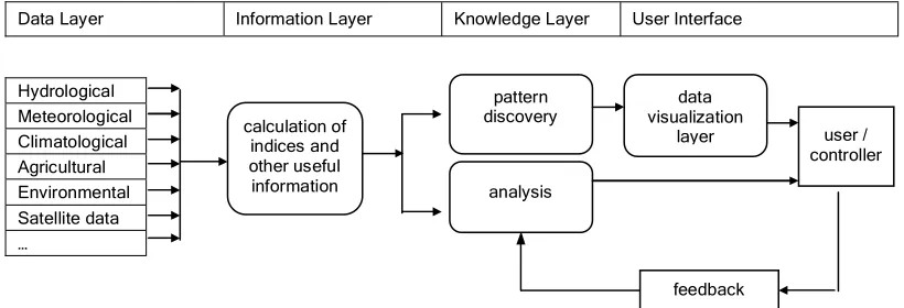
A simplified flowchart for the agro-hydrological system look like as shown below:
Data Layer Information Layer Knowledge Layer User Interface
Hydrological Meteorological Climatological Agricultural Environmental Satellite data …
Fig. 3: A simplified hypothetical flow chart for the agro-hydrological system
8. Discussion and conclusions
In this paper, a few challenges especially related to clustering spatial data are pointed out. There exist some problems that k-means method cannot tackle, especially for dealing with spatial and complex data. Among these, the important issues/problems that need to be addressed are: i) non-linear separability of data in
input space, ii) outliers and noise, iii) auto-correlation in spatial data, iv) high dimensionality of data. The strengths of kernel methods are outlined, which are helpful for clustering complex and high dimensional data that is non-linearly separable in input space. Two of the currently proposed kernel based algorithms are reviewed and the related research issues are identified. Both [2, 4] are computationally very intensive, unable to handle large datasets and have no
user / controller data
visualization layer calculation of
indices and other useful
information analysis pattern discovery
mechanism to deal with autocorrelation in the spatial data. The method proposed in [2] is not feasible to handle high dimensional data due to computational overheads, whereas the convergence of [4] is an open problem. With regard to addressing these problems, we presented weighted kernel k-means incorporating spatial constraints. The proposed algorithm has the mechanism to handle spatial autocorrelation, noise and outliers in the spatial data. We are getting promising results on our test data sets. It is very much hoped that the algorithm would prove to be robust and effective for spatial (climate) data analysis. In future we plan to investigate the estimation of optimal number of clusters automatically.
References
[1] M.N. Ahmed, S.M. Yamany, N. Mohamed, A.A. Farag and T. Moriarty. A modified fuzzy C-means algorithm for bias field estimation and segmentation of MRI data. IEEE Trans. on Medical Imaging, vol. 21, pp.193–199, 2002.
[2] A. Ben-Hur, D. Horn, H. Siegelman, and V. Vapnik. Support vector clustering. Journal of Machine Learning Research 2, 2001.
[3] F. Camastra. Kernel Methods for Unsupervised Learning. PhD thesis, University of Genova, 2004.
[4] F. Camastra, A. Verri. A Novel Kernel Method for Clustering. IEEE Trans. on Pattern Analysis and Machine Intelligence, vol 27, pp 801-805, May 2005.
[5] J. H. Chen and C. S. Chen. Fuzzy kernel perceptron. IEEE Trans. Neural Networks, vol. 13, pp. 1364–1373, Nov. 2002.
[6] N. Cristianini and J.S.Taylor. An Introduction to Support Vector Machines. Cambridge Academic Press, 2000.
[7] I.S. Dhillon, Y. Guan, B. Kulis. Kernel kmeans, Spectral Clustering and Normalized Cuts. KDD 2004.
[8] C. Ding and X. He. K-means Clustering via Principal Component Analysis. Proc. of Int'l Conf. Machine Learning (ICML 2004), pp 225–232, July 2004.
[9] M. Girolami. Mercer Kernel Based Clustering in Feature Space. IEEE Trans. on Neural Networks. Vol 13, 2002.
[10] R.M. Gray. Vector Quantization and Signal Compression. Kluwer Academic Press, Dordrecht, 1992.
[11] J. Han, M. Kamber and K. H. Tung. Spatial Clustering Methods in Data Mining: A Survey. Harvey J. Miller and Jiawei Han (eds.), Geographic Data Mining and Knowledge Discovery, Taylor and Francis, 2001.
[12] S.P. Lloyd. An algorithm for vector quantizer design. IEEE Trans. on Communications, vol. 28, no. 1, pp. 84–95, 1982.
[13] M.N. Md. Sap, A. Majid Awan. Weighted Kernel K-Means Algorithm for Clustering Spatial Data. Journal of
Information Technology, University Technology Malaysia, Vol 16 (2), pp. 137–156, Dec 2004.
[14] V. Roth and V. Steinhage. Nonlinear discriminant analysis using kernel functions. In Advances in Neural Information Processing Systems 12, S. A Solla, T. K. Leen, and K.-R. Muller, Eds. MIT Press, 2000, pp. 568–574.
[15] D.S. Satish and C.C. Sekhar. Kernel based clustering for multiclass data. Int. Conf. on Neural Information Processing , Kolkata, Nov. 2004.
[16] B. Scholkopf and A. Smola. Learning with Kernels: Support Vector Machines, Regularization, Optimization, and Beyond. MIT Press, 2002.
[17] B. Scholkopf, A. Smola, and K. R. Müller. Nonlinear component analysis as a kernel eigenvalue problem. Neural Comput., vol. 10, no. 5, pp. 1299–1319, 1998.
[18] S. Shekhar, P. Zhang, Y. Huang, R. Vatsavai. Trends in Spatial Data Mining. As a chapter in Data Mining: Next Generation Challenges and Future Directions, H. Kargupta, A. Joshi, K. Sivakumar, and Y. Yesha (eds.), MIT Press, 2003
[19] V.N. Vapnik. The Nature of Statistical Learning Theory. Springer-Verlag, New York, 1995.
[20] V.N. Vapnik. Statistical Learning Theory. John Wiley & Sons, 1998 .
[21] L. Xu, J. Neufeld, B. Larson, D. Schuurmans. Maximum Margin Clustering. NIPS 2004.
[22] P. Zhang, M. Steinbach, V. Kumar, S. Shekhar, P-N Tan, S. Klooster, and C. Potter. Discovery of Patterns of Earth Science Data Using Data Mining. As a Chapter in Next Generation of Data Mining Applications, J. Zurada and M. Kantardzic (eds), IEEE Press, 2003.
[23] I.S. Dhillon, J. Fan, and Y. Guan. Efficient clustering of very large document collections. In Data Mining for Scientific and Engineering Applications, pp.357–381. Kluwer Academic Publishers, 2001.
[24] I.S. Dhillon, Y. Guan, B. Kulis. Kernel kmeans, Spectral Clustering and Normalized Cuts. KDD 2004.
[25] C. Elkan. Using the triangle inequality to accelerate k-means. In Proc. of 20th ICML, 2003.