Networks for Monaural Audio Source Separation
Emad M. Grais, Hagen Wierstorf, Dominic Ward, and Mark D. Plumbley Centre for Vision, Speech and Signal Processing, University of Surrey, Guildford, UK.
{grais,dominic.ward,m.plumbley}@surrey.ac.uk,[email protected]
Abstract. In deep neural networks with convolutional layers, all the neurons in each layer typically have the same size receptive fields (RFs) with the same resolution. Convolutional layers with neurons that have large RF capture global information from the input features, while layers with neurons that have small RF size capture local details with high resolution from the input features. In this work, we introduce novel deep multi-resolution fully convolutional neural networks (MR-FCN), where each layer has a range of neurons with different RF sizes to extract multi-resolution features that capture the global and local information from its input features. The proposed MR-FCN is applied to separate the singing voice from mixtures of music sources. Experimental results show that using MR-FCN improves the performance compared to feedforward deep neural networks (DNNs) and single resolution deep fully convolutional neural networks (FCNs) on the audio source separation problem.
Keywords: Multi-resolution features extraction, fully convolutional neu-ral networks, deep learning, audio source separation, audio enhancement.
1
Introduction
Monaural audio source separation (MASS) aims to separate audio sources from a single (mono) audio mixture [20]. A variety of deep neural networks with convolutional layers have been used recently to tackle this problem [2, 6, 11, 12, 18]. One of the main differ-ences in those works relies on using either fully convolutional neural networks (FCN), where all the network layers are convolutional layers, or networks where some of the layers are convolutional and others are fully connected layers. The common aspect in those works is that each convolutional layer is composed of a set of neurons/filters that have the same receptive field (RF) size. The RF is the field of view of a neuron (filter in the FCN case) in a certain layer in the network [21]. In fully connected deep neural networks (DNNs), the output of each neuron in a certain layer depends on the entire input to that layer, while the output of a neuron in a convolutional layer only depends on a region of the input: this region is the RF for that neuron. The RF size is a crucial issue in many audio and visual tasks, as the output must respond to areas with sizes correspond to the sizes of the different objects or patterns in the input data to extract useful information/features about each object [21]. The size of the RF equals the size of the filters in a convolutional layer. A large filter size captures the global structure of its input features [9, 17], while a small filter size captures the local details with high resolution but it does not capture the global structure of its input features. Intuitively,
it might be useful to have sets of filters that can extract both the global and local de-tails from the input features in each layer. This might be useful in the MASS problem, since the input signal is a mixture of different audio sources and useful features can be extracted for certain sources in certain time-frequency resolutions which may differ from one source to another [16].
The concept of extracting multi-resolution features has been proposed recently for many signal processing applications with different ways of extracting and combining the multi-resolution features from the input data [5, 9, 13, 23]. In this paper, we introduce a novel multi-resolution fully convolutional neural network (MR-FCN) model for MASS, where each layer in the MR-FCN is a convolutional layer that is composed of different sets of filters. All filters within a given set have the same size, which is different to the size of filters in other sets in the same layer. Thus, in each layer there are sets of filters with large and small sizes, which allows each layer to extract multi-resolution features that capture the global and local information from its input data. We believe that this is the first time that a deep neural network has been proposed with each layer composed of multi-resolution filters that extract multi-resolution features from the layer before, and the first time that the concept of extracting multi-resolution features has been used for MASS. The inputs and outputs of the MR-FCN are two-dimensional (2D) segments from the magnitude spectrogram of the mixed and target source signals respectively. The MR-FCN is trained to extract useful spectro-temporal features and patterns in different time-frequency resolutions to separate the target source from the input mixture.
This paper is organized as follows: Section 2 shows a brief introduction about the FCN and the proposed MR-FCN. The proposed approach of using MR-FCN for MASS is presented in Section 3. Section 4 introduces our experiment and discusses the results, and Section 5 draws conclusions and directions for future work.
2
Multi-resolution fully convolutional neural networks
In this section we first give an introduction about the fully convolutional neural network (FCN) then we introduce the proposed MR-FCN.
2.1 Fully convolutional neural networks (FCNs)
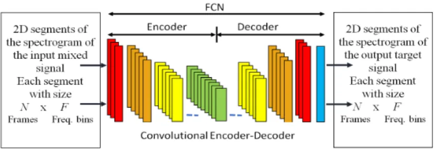
The FCN model that we propose here (Fig. 1) is somewhat similar to the convolutional denoising encoder-decoder (auto-encoder) network that was used in [6,15], but without using either down-sampling (pooling) or up-sampling. The encoder part in the FCN is composed of repetitions of a convolutional layer and an activation layer. The decoder part consists of repetitions of a transpose convolutional layer [4] and an activation layer. Each layer in the FCN consists of a single set of filters with the same size to extract feature maps from its input layer, and the activation layer imposes nonlinearity to these feature maps.
The FCN can be trained from corrupted input signals and the encoder part is used to extract noise robust features that the decoder can use to reconstruct a cleaned-up version of the input data [15, 24]. In MASS, the input mixed signal can be seen as a sum of the target source that needs to be separated and background noise (the other sources in the mixture). The input and output data of the FCN are 2D signals (magnitude spectrograms) and the filtering is a 2D operator.
Fig. 1:Overview structure of a FCN that separates one target source from the mixed signal. Each layer consists of a single set of filters with the same size followed by an activation function. The sets of filters in the input and output layers have large filter sizes and small number of filters. The number of filters increases and the size decreases when getting further from the input and output layers [15]. There is symmetric in the filter sizes and numbers of filters between the encoder and decoder sides.
2.2 Multi-resolution FCN
Each layer in the FCN in Fig.1 is composed of one set of filters that have the same RF size. The size of the RF is a very important parameter, as the output of each filter should respond to areas with sizes correspond to the sizes of the different objects/patterns in the input to extract useful information/features from the input data [21]. For example, if the size of the RF of a filter is much bigger than the size of the input pattern, the filter may capture blurred features from the input patterns, while if the RF of a unit is smaller than the size of the input patterns, the output of the filter loses the global structure of the input patterns [21].
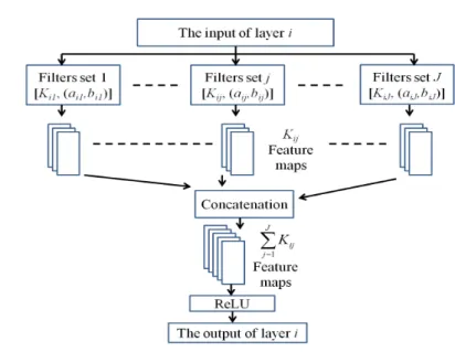
In audio source separation problems, the spectrogram of the input mixed signal usually contains different combinations of different spectro-temporal patterns from dif-ferent audio sources. There is a unique set of patterns associated with each source in the spectrogram of their mixture, and these patterns appear in different spectro-temporal sizes [1]. So, to use the FCN to extract useful information about the individual sources in the spectrogram of their mixture, it might be useful to use filters with different RF sizes in each layer, where the different RF sizes are proportional to the diversity of the spectro-temporal sizes of the patterns in the spectrogram. Bearing these issues in mind, we propose a MR-FCN which is the FCN shown in Fig.1 but with multi-resolution fil-ters (filfil-ters with different sizes) in each layer. Thus, each layer in the MR-FCN has sets of 2D filters. The filters in one set have the same size which is different to the sizes of the filters in all other sets in the same layer. Each set of filters generates fea-ture maps with certain time-frequency resolution. Fig. 2 shows the detailed strucfea-ture for each layer in the MR-FCN. Each layer in the MR-FCN generates multi-resolution features from its input features and also combines the multi-resolution features from the previous layers to generate accurate patterns that compose the structure of the underlying data.
Fig. 2:Overview of the proposed structure of each layer of the MR-FCN. WhereKij denotes the number of filters with sizeaij×bij in setjin layeri,aij is the dimension in the time direction of the filters, andbijis the dimension in the frequency direction of the filters in setjand layeri. The filters in different sets have different sizes and the filters within a set have the same size. Each setj in layerigeneratesKij feature maps. The number of feature maps that each layerigenerates equal to the sum of the number of feature maps that all the sets in layerigenerate (PJ
j=1Kij). ReLU denotes a rectified linear unit as an activation function.
3
MR-FCN for MASS
Given a mixture of L sources asy(t) =PL
l=1sl(t), the aim of MASS is to estimate
the sourcessl(t), ∀l, from the mixed signaly(t) [20]. We work here in the short-time
Fourier transform (STFT) domain. Given the STFT of the mixed signaly(t), the main goal is to estimate the STFT of each source in the mixture.
In this work, we propose to use as many MR-FCN as the number of sources to be separated from the mixed signal. Each MR-FCN sees the mixed signal as a combina-tion of its target source and background noise. The main aim of each MR-FCN is to separate its corresponding target source from the other background sources that exist in the mixed signal. This is a challenging task since each MR-FCN deals with highly nonstationary background noise (other sources in the mixture). The inputs and outputs of the MR-FCNs are 2D-segments from the magnitude spectrograms of the mixed and target signals respectively. Therefore, the MR-FCNs span multiple spectral frames to capture multi-resolution spectro-temporal characteristics for each source. The number of spectral frames that each segment has isN and the number of frequency bins isF. In this work,F is the dimension of the whole spectral frame.
3.1 Training the MR-FCNs for source separation
We train each MR-FCN to map the magnitude spectrogram of the input mixture into the magnitude spectrogram of its corresponding target source. Let us assume that we have training data for the mixed signals and their corresponding clean/target sources. LetYtr be the magnitude spectrogram of the mixed signal and Sl be the magnitude
spectrogram of the target sourcel. The subscript “tr” denotes the training data. The MR-FCN that separates sourcelfrom the mixture is trained to minimize the following cost function:
Cl=
X
n,f
(Zl(n, f)−Sl(n, f))2 (1)
where Zlis the actual output of the last layer of the MR-FCN of source l,Sl is the
reference target output for sourcel, and n andf are the time and frequency indices respectively. The input to all the MR-FCNs is the magnitude spectrogramYtr of the
mixed signal. The input and output instants of the MR-FCNs are 2D-segments, where each segment is composed ofN consecutive spectral frames taken from the magnitude spectrograms. This allows each MR-FCN to learn multi-resolution spectro-temporal patterns for its corresponding target source.
3.2 Testing the MR-FCNs for source separation
After training a MR-FCN for each source we wish to separate from the mixed signal, the magnitude spectrogram Y of the mixed signal is passed through all the trained MR-FCNs. The output of the MR-FCN of sourcelis the estimateS˜lof the magnitude
spectrogram of sourcel. The time domain estimate˜sl(t) is computed using the inverse
STFT of the estimateS˜land the phase of the STFT of the input mixture.
4
Experiments
We applied our proposed MASS using MR-FCN approach to separate the singing voice/vocal sources from a group of songs from the SiSEC-2015-MUS-task dataset [14]. The dataset has 100 stereo songs with different genres and instrumentations. To use the data for the proposed MASS approach, we converted the stereo songs into mono by computing the average of the two channels for all songs and sources in the data set. Each song is a mixture of vocals, bass, drums, and a group of other musical instruments. We used one MR-FCN to separate the vocal from each song.
The first 50 songs in the dataset were used as training and validation datasets, and the last 50 songs were used for testing. The data were sampled at 44.1 kHz. The magnitude spectrograms for the data were calculated using the STFT with Hanning window size 2048 points and hop size of 512 points. The FFT was computed with 2048 points and the first 1025 were used as features since they include the conjugate of the remaining points.
The quality of the separated sources was measured using the source to distortion ratio (SDR), source to interference ratio (SIR), and source to artifact ratio (SAR) [19]. SIR indicates how well the sources are separated based on the remaining interference between the sources after separation. SAR indicates the artifacts caused by the separa-tion algorithm in the estimated separated sources. SDR measures the overall distorsepara-tion
(interference and artifacts) of the separated sources. The SDR values are usually con-sidered as the overall performance evaluation for any source separation approach [19]. Achieving high SDR, SIR, and SAR indicates good separation performance.
We compared the performance of using the proposed MR-FCN model with the per-formance of using feedforward deep neural networks (DNNs) and the (single-resolution) FCN for separating the vocal signals from each song in the test set. For the input and output data for the MR-FCN and FCN, we chose the number of spectral frames in each 2D-segment to be 15 frames. This means the dimension of each input and output instant for the MR-FCN and FCN is 15 (time frames)×1025 (frequency bins) as in [6]. Thus, each input and output instant (the 2D-segments from the spectrograms) spans around 209 ms of the waveforms of the data. Each input and output instant of the DNN is a single frame of the magnitude spectrograms of the input and output signals respectively.
FCN and MR-FCN model summary
The input/output data with size 15 frames and 1025 frequency bins
Layer number FCN MR-FCN 1 Conv2D[26,(15,39)] set 1 Conv2D[12,(15,39)] set 2 Conv2D[6,(9,19)] set 3 Conv2D[6,(5,5)] 2 Conv2D[42,(9,19)] set 1 Conv2D[8,(15,39)] set 2 Conv2D[22,(9,19)] set 3 Conv2D[8,(5,5)] 3 Conv2D[66,(5,5)] set 1 Conv2D[12,(15,39)] set 2 Conv2D[12,(9,19)] set 3 Conv2D[32,(5,5)] 4 Conv2D[42,(9,19)] set 1 Conv2D[8,(15,39)] set 2 Conv2D[22,(9,19)] set 3 Conv2D[8,(5,5)] 5 Conv2D[26,(15,39)] set 1 Conv2D[12,(15,39)] set 2 Conv2D[6,(9,19)] set 3 Conv2D[6,(5,5)] 6 Conv2D[1,(15,1025)] Conv2D[1,(15,1025)]
Total number of parameters 1,784,027 1,755,321
Table 1:The filter specifications and the number of filters in each layer of the FCN and MR-FCN. For example “Conv2D[26,(15,39)]” denotes 2D convolutional layer with 26 filters and the size of each filter is 15×39 where 15 is the size of the filter in the time-frame direction and 39 in the frequency direction of the spectrogram.
4.1 Choosing the parameters of the models
As in many deep learning models, there are many parameters in the proposed MR-FCN to be chosen (number of layers, filter size, and the number of filters in each set) and usually these choices are data and application dependent. Choosing the parameters for the FCN is also not easy. In this work, we follow the same strategy as in [15] where the size of the filters decreases but the number of the filters increases as we progress through the layers of the encoder part. In contrast, we use fewer filters of increasing size as we develop through the decoder part. For MR-FCN, the number and size of the filters in each set in each layer are need to be decided. We restricted ourselves in this work to use only three sets of filters for the whole network. The first set with size 15×39 (each filter in this set spans around 209 ms of the waveforms and a band of frequencies
around 840 Hz in the spectrogram), the second set with size 9×19 (each filter in this set spans around 139 ms of the waveforms and a band of frequencies around 409 Hz in the spectrogram), and the third set with size 5×5 (each filter in this set spans around 93 ms of the waveforms and a band of frequencies around 108 Hz in the spectrogram). Which means each layer has sets of filters with three different time-frequency resolutions. Also following the same concept in [15] for choosing the number of filters, the layers towards the input and output layers have more filters with large size than the layers in the middle. The layers in the middle have more filters in the set with small filter size than the layers toward the input and output layers. For example, the first layer in MR-FCN has a set of 12 filters with size 15×39, a set of 6 filters with size 9×19, and a set of 6 filters with size 5×5. Thus, the first layer generates 24 feature maps with three different resolutions. Each feature map is 15×1025 (the same size of the input and output segments).
To attempt to make a fair comparison between the proposed MR-FCN model and the FCN, we adjusted the number of filters and their sizes in each layer of both models to have total number of parameters in both models close to each other as shown in Table 1. Table 1 shows the number of layers, the number of filters in each layer, and the size of the filters for the FCN and MR-FCN models. The DNN has three hidden layers, and each hidden layer has 1025 nodes. The parameters of the DNN are tuned based on our previous work on the same dataset [7]. The rectified linear unit (ReLU) is used as the activation function for all the neural networks in this work. The DNN here has 4,206,600 parameters, the FCN has 1,784,027 parameters, and the MR-FCN has 1,755,321 parameters. This means the MR-FCN has the smallest number of parameters compared to the FCN and the DNN.
The parameters for all the networks were initialized randomly. They were trained using backpropagation with gradient descent optimization using Adam [10] with pa-rameters: β1 = 0.9,β2 = 0.999, = 10−8, a batch size 100, and an initial learning rate of 0.0001 which was reduced by a factor of 10 when the values of the cost func-tion ceased to decrease on the validafunc-tion set for 3 consecutive epochs. The maximum number of epochs was 100. We implemented our proposed algorithm using Keras with Tensorflow backend [3].
4.2 Results
Fig.3 shows boxplots of the SDR (a), SIR (b), and SAR (c) as measured on the vocals separated using three different deep learning models, namely DNN, FCN, and MR-FCN. The figure also shows the SDR and SIR values of the target vocal source in the mixed signal (denoted as Mix in Fig.3). We did not show the SAR of the mixed signal because it is usually very high. From the figure we can see that the vocal signals in the input mixed signal (denoted as Mix in Fig.3) have very low SDR and SIR values, which shows that we are dealing with a very challenging source separation problem.
As can be seen from Fig.3, the three methods perform well on the SDR, SIR, and SAR values of the separated vocal signals. The proposed MR-FCN model outperforms the DNN and slightly outperforms the FCN in all measurements.
In the following, we consider the difference between a pair of models statistically significant if p < 0.05, Wilcoxon signed-rank test [22] and Bonferroni corrected [8]. Based on the shown results in Fig. 3, the difference between each pair of models for all the shown results of SDR is statistically significant with P values as follows. For SDR: P(DNN,FCN) = 1.12×10⁻⁷, P(DNN,MR-FCN) = 1.22×10⁻⁷, and
Mix DNN FCN MR-FCN -15 -10 -5 0 5 SDR in dB (a) SDR in dB Mix DNN FCN MR-FCN -15 -10 -5 0 5 10 15 SIR in dB (b) SIR in dB DNN FCN MR-FCN -4 -2 0 2 4 6 8 10 SAR in dB (c) SAR in dB
Fig. 3:(a) The SDR, (b) the SIR, and (c) the SAR (values in dB) for the separated vocal signals of using: deep fully connected feedforward neural networks (DNNs), deep fully convolutional neural networks (FCNs), and the proposed multi-resolution fully convolutional neural networks (MR-FCN). ”Mix“ denotes the input mixed signal.
P(FCN,MR-FCN) = 0.004. For SIR: P(DNN,FCN) = 0.9, P(DNN,MR-FCN) = 0.04, and P(FCN,MR-FCN) = 4.9×10⁻⁴. For SAR: P(DNN,FCN) = 2.2×10⁻⁷,
P(DNN,MR-FCN) = 3.8×10⁻⁷, and P(FCN,MR-FCN) = 2.02. In particular, the MR-FCN is statistically significantly better than FCN in SDR and SIR (p <0.05), and statistically significantly better than DNN in all the measurements.
4.3 Discussion
Although the difference between the results of MR-FCN and FCN is statistically sig-nificant (p <0.05) in SDR and SIR, the improvement of using MR-FCN over FCN is marginal: the mean difference between MR-FCN and FCN is less than 1 dB in SDR and SIR. We believe that the filter sizes and the number of filters in each set should be refined to yield further improvements. These choices could be associated with the band of frequencies that each source covers in the input mixtures. Note that, FCN in this experiment has 28,706 more parameters than MR-FCN. In our future work, we will investigate different choices for the filter sizes and number of filters in each layer and each set.
5
Conclusions
In this work we proposed a new approach for monaural audio source separation (MASS). The new approach is based on using deep multi-resolution fully convolutional neural networks (MR-FCN). The MR-FCN learns multi-resolution patterns for each source and uses this information to separate the related components of each source from the mixed signal. The experimental results indicate that using MR-FCN for MASS is a promising approach and with a few number of parameters can achieve better results than the feedforward neural networks and the single resolution fully convolutional neu-ral networks.
In our future work, we will investigate the possibility of applying the MR-FCN on raw audio data (time domain signals) to extract multi-resolution time-frequency features that can represent the input data better than the STFT features. Some audio sources require higher resolution in time than in frequency, and other audio sources re-quire the opposite resolution of that. By applying MR-FCN on the raw audio data, we hope to extract useful features for each source according to its preferred time-frequency resolution which can improve the performance of many audio signal processing ap-proaches.
ACKNOWLEDGMENT
This work is supported by grant EP/L027119/2 from the UK Engineering and Physical Sciences Research Council (EPSRC).
References
1. A. Klapuri, M.D.: Signal Processing Methods for Music Transcription. Springer (2007)
2. Chandna, P., Miron, M., Janer, J., Gomez, E.: Monoaural audio source separation using deep convolutional neural networks. In: Proc. LVA/ICA. pp. 258–266 (2017) 3. Chollet, F.: Keras, https://github.com/fchollet/keras (2015)
4. Dumoulin, V., Visin, F.: A guide to convolution arithmetic for deep learning. In: arXiv:1603.07285 (2016)
5. Espi, M., Fujimoto, M., Kinoshita, K., Nakatani, T.: Exploiting spectro-temporal locality in deep learning based acoustic event detection. EURASIP Journal on Audio, Speech, and Music Processing 26, 1–12 (2015)
6. Grais, E.M., Plumbley, M.D.: Single channel audio source separation using convo-lutional denoising autoencoders. In: Proc. GlobalSIP (2017)
7. Grais, E.M., Roma, G., Simpson, A.J.R., Plumbley, M.D.: Combining mask esti-mates for single channel audio source separation using deep neural networks. In: Prec. InterSpeech (2016)
8. Hochberg, Y., Tamhane, A.C.: Multiple Comparison Procedures. John Wiley and Sons (1987)
9. Kawahara, J., Hamarneh, G.: Multi-resolution-tract CNN with hybrid pretrained and skin-lesion trained layers. In: Proc. MICCAI MLMI. vol. 10019, pp. 164–171 (2016)
10. Kingma, D.P., Ba, J.: Adam: A method for stochastic optimization. In: Proc. arXiv:1412.6980 and presented at ICLR (2015)
11. Lim, W., Lee, T.: Harmonic and percussive source separation using a convolutional auto encoder. In: Proc. EUSIPCO (2017)
12. Miron, M., Janer, J., Gomez, E.: Monaural score-informed source separation for classical music using convolutional neural networks. In: Proc. ISMIR (2017) 13. Naderi, N., Nasersharif, B.: Multiresolution convolutional neural network for robust
speech recognition. In: Proc. ICEE (2017)
14. Ono, N., Rafii, Z., Kitamura, D., Ito, N., Liutkus, A.: The 2015 signal separation evaluation campaign. In: Proc. LVA/ICA. pp. 387–395 (2015)
15. Park, S.R., Lee, J.W.: A fully convolutional neural network for speech enhance-ment. In: Proc. Interspeech (2017)
16. Simpson, A.J.: Time-frequency trade-offs for audio source separation with binary masks. In: arXiv:1504.07372 (2015)
17. Tang, Y., Mohamed, A.: Multiresolution deep belief networks. In: Proc. AISTATS (2012)
18. Venkataramani, S., Smaragdis, P.: End-to-end source separation with adaptive front-ends. In: Proc. WASPAA (2017)
19. Vincent, E., Gribonval, R., Fevotte, C.: Performance measurement in blind audio source separation. IEEE Trans. on Audio, Speech, and Language Processing 14(4), 1462–69 (Jul 2006)
20. Virtanen, T.: Monaural sound source separation by non-negative matrix factor-ization with temporal continuity and sparseness criteria. IEEE Trans. on Audio, Speech, and Language Processing 15, 1066–1074 (Mar 2007)
21. Wenjie, L., Yujia, L., Raquel, U., Richard, Z.: Understanding the effective receptive field in deep convolutional neural networks. In: Proc. NIPS. pp. 4898–4906 (2016) 22. Wilcoxon, F.: Individual comparisons by ranking methods. Biometrics Bulletin
1(6), 80–83 (1945)
23. Xue, W., Zhao, H., Zhang, L.: Encoding multi-resolution two-stream CNNs for action recognition. In: Proc. ICONIP. pp. 564–571 (2016)
24. Zhao, M., Wang, D., Zhang, Z., Zhang, X.: Music removal by convolutional denois-ing autoencoder in speech recognition. In: proc. APSIPA (2016)