Measures of Surprise and Threshold
Selection
in Extreme Value Statistics
Professor : Anthony C. Davison Supervisor : Scott Sisson
Irene Vicari January 15, 2010
Introduction 3
1 Measures of Surprise 5
1.1 Weaver's and Good's Surprise Indices . . . 6
1.2 Prior Predictive p-values . . . 8
1.3 Posterior Predictive p-values . . . 9
1.4 Other Proposals to Measure Surprise . . . 10
1.5 Relative Maximized and Expected Measures of Surprise . . . 12
1.6 Conditional Predictive Distribution . . . 13
1.6.1 Through one-to-one Transformation ofX . . . 14
1.6.2 Ideal Choice ofU . . . 15
1.6.3 Asymptotic Independence . . . 15
1.6.4 Suciency for the Nuisance Parameter . . . 16
1.6.5 An Attractive Choice ofU . . . 16
1.6.6 Computational Issues . . . 16
1.7 Calibration of p-values . . . 19
2 Threshold Selection for the Generalized Pareto Distribution 22 2.1 Generalized Extreme Value Model . . . 22
2.2 Threshold Exceedance Model . . . 24
2.3 Threshold Selection . . . 25
2.3.1 Parameter Stability . . . 26
2.3.2 Mean Residual Life Plot . . . 26
2.3.3 Bayes Estimation . . . 27
3 Simulation Study 31 3.1 Posterior Predictive p-values . . . 31
3.1.1 Uniform and Generalized Pareto Data . . . 33
3.1.3 Generalized Pareto Data . . . 43
3.2 Prior Predictive p-values . . . 46
3.2.1 Laplace Approximation . . . 46
Conclusion 49
Measures of surprise have been recently studied in statistics. This new con-cept can be used as the rst exploratory tool to verify if a model under the null hypothesis ts appropriately. As no alternative models are necessary, the use of the measures of surprise is considered very simple. At the same time, this new alternative to test the goodness of a model cannot replace the full Bayesian analysis.
The aim of this project is threshold selection for threshold models. The estimate of the threshold could be investigated by using the measures of surprise. The reason is that no alternative models are specied for non-extreme data, for which the distribution in non-extreme value theory is unknown, and thus the surprise would be a credible tool.
In order to quantify the measures of surprise, predictive marginal likeli-hoods are computed. The purpose of these quantities is to observe if data are surprising under a given model. For this reason we calculate the p-values with respect to the predictive marginal likelihoods. Section 1 describes all these measures and gives their respectively p-values.
In Section2the basic concepts of the extreme value theory are reviewed. Firstly, the generalized extreme value distribution is denite to allow the introduction of the generalized Pareto distribution and its properties. Fi-nally, dierent methods to estimate the threshold u of a dataset having a generalized Pareto distribution are studied.
In order to analyse the measures of surprise more profoundly, a simulation study is carried out in Section 3 and two particular predictive marginal likelihoods are considered: the posterior and the prior predictive marginal likelihoods. Given dierent datasets, the aim is to estimate the thresholdu using these two measures of surprise.
Three dierent samples (uniform and generalized Pareto data, gamma and generalized Pareto data, generalized Pareto data only) are generated and the behaviour of the posterior predictive measures of surprise is anal-ysed. Because of numerical reasons, we use the mean of the generalized
Pareto density of each observation rather than the product of the densities. This approximation allows to obtain some interesting results which give the estimation of the true thresholdu.
The prior predictive measures of surprise are estimated using the Laplace approximation method. Once more, the likelihood is replaced by the mean of the densities for numerical reasons. For this approach the study is carried out only for the sample generated by uniform and generalized Pareto data.
Finally, we discuss the results and the problems that we have had con-cerning some computations of the measures of surprise. Furthermore, some suggestions are also presented in order to improve and ride over these com-putational diculties.
Measures of Surprise
Once a (null) model (or hypothesis)H0 is formulated andxobs is observed, are data surprising? (Bayarri and Berger, 1997). In Statistics this is a very old question and to answer it we introduce the notion of measure of surprise.
Denition 1 (Bayarri and Berger (1997)). The measure of surprise in-dicates the need of modication of the model. It gives the incompatibility degree of data with an hypothesized model H0 without any reference to
alternative models.
This means that there is no way to compare the model under the null hypothesis without any other models.
The use of the measure of surprise is considered extremely interesting because it is very simple. No alternative models with their priors over their parameters exist. A surprise analysis cannot replace a full Bayesian one but it plays an important role as exploratory tool. This means that if the data xobs can be explained by H0, we might not need to carry out also
the full analysis which corresponds to compare the null model with dierent alternative models with their associated priors over their parameters. On the other hand, if xobs is surprising, then we have to indicate an alternative
model toH0 and we have to carry out a Bayesian analysis without rejecting
directly the model under the null hypothesis.
Under it we usually haveX ∼f(x|θ)andθ∼π(θ)but since there is no
explicit H1, no prior is assigned. Once we introduce an alternative model,
we haveX ∼f1(x|η) andη ∼π1(η).
We often use a statistic T(X) to investigate the compatibility of the
distribution under H0 will be f(t | θ) = f(t). The best-known way to
measure the compatibility of the model is p-values or tail area probabilities dened byBayarri and Morales (2003) as follows,
p= Prf(·){T(X)≥T(xobs)}.
On the other hand, it is extremely rare to know the parameterθ. There-fore, in the next sections we will focus dierent kind of probability distribu-tions used to compute the p-values.
1.1 Weaver's and Good's Surprise Indices
The surprise index is based on the probability f(xobs) of observing data
that eventually occurred. Weaver underlined that a small probability is not necessary surprising unless it is small if compared with the probabilityf(x)
of the other possible results (Weaver(1948) and Weaver(1963)).
The basic idea consists in the comparison betweenf(xobs) and the
aver-age (expected) probability. Let X be a random variable or vector having a discrete distribution. Letx1, x2, . . .have probabilitiesf1, f2, . . .respectively.
Then the surprise index associated with the observed valuexobs is
λ1= E{f(X)} Pr{X =xobs} = P ifi2 fobs , whereP
ifi2 corresponds to the Gini's homogeneity index (Good,1988). The surprise index generalized to continuous random variables is
λ1= E{f(X)} Pr{X=xobs} = R f(x)2dx f(xobs) . (1.1)
We notice that the Weaver's index (1.1) is multiplicative. This means that ifX and Y are independent random variables, then
λ1(xobs, yobs) =λ1(xobs)λ1(yobs). (1.2)
When we use Weaver's surprise index, two possible diculties could arise. The rst one concerns its invariance: it is invariant only under linear trans-formations. The second one refers to the standard chosen to compare the observedf(xobs)with its expected valueE{f(X)}which might be considered
somewhat arbitrary. A single-parameter generalization of (1.1) is suggested byGood(1953) andGood(1956) that would also possess the property (1.2).
These measures of surprise comparef(xobs)with some sort of geometric
expectation. Two dierent cases are considered. First, forc >0 the index is
λc= [E{f(X)
c}]1/c
f(xobs)
. (1.3)
Second, the limiting case, asc→0 gives
λ0=
exp[E{log(f(X))}]
f(xobs) . (1.4)
Notice that forc= 1, equation (1.3) corresponds to Weaver's index.
Another generalization has been proposed byGood(1988),
λ0 =
φ−1[E{φ(f(X))}]
f(xobs)
.
In this caseφis a monotonic increasing function that is multiplicative only in the case in whichφ is a power or logarithm (so that it reduces to either (1.3) or (1.4)).
If an additive index is required, it could be possible to use the loga-rithmic surprise index. This was proposed by Good (1956) using the logarithm of (1.3),
Λc= log(λc), c≥0.
This index has many connections with information theory. In particular,
Λc + log{f(xobs)} is also called Renyi's generalized entropy (Renyi,
1961). Then, we have
Λ1 = log[E{f(X)}]−log{f(xobs)} Λ0 = E[log{f(X)}]−log{f(xobs)}.
Measuresλ1,λ0 andΛ1,Λ0 are considered to be the most natural by Good
basing on properties of the expected indices of surprise before the experiment is performed.
We need to detail the distribution of the observations underH0if we want
to compute these indices. Unfortunately it is not always possible. Then we introduce tail areas or Bayesian p-values which allow to compute the measure of surprise, as we work on suitable predictive distributions.
1.2 Prior Predictive p-values
UnderH0 data are distributed as X∼f(x|θ) and the prior distribution is
θ∼π(θ). Then the prior predictive distribution for Bayesians is
m(x) =
Z
f(x|θ)π(θ)dθ, (1.5)
which is the natural tool to quantify surprise. Equation (1.5) corresponds to the probability of observing datax. This means that a small value of m(x)
would indicate data that are unlikely to be observed. If the observationxobs
produces a small m(xobs), then there is evidence of surprise.
In order to understand how small ism(xobs), we have to compare it with
some standard. For example, we comparem(xobs)with some possiblem(x)
(see Section1.5). Box(1980) proposed to compute the associated tail area ofm(xobs)in the prior predictivem(x)to measure the smallness ofm(xobs).
He dened
α= Prm(·){m(X)< m(xobs)}
as an overall predictive check of a given model, where the probability is computed with respect to the prior predictive distribution (1.5). So we can use1−αor 1/αas measures of surprise. In the same way, we can compute the surprise for some functionsD(xobs) by
Prm(·){m(D(X))< m(D(xobs))}. (1.6)
As these measures of surprise are very close to classical p-values, they violate the conditionality principle and the likelihood principle, too. These probabilities are also based on values of X that provide a much stronger evidence against the null model than the observed one, so we obtain an exaggerated measure of surprise. Another negative feature is that the prior predictive p-values are not invariant under one-to-one transformation (see the example ofEvans (1997)).
To remove some of these diculties, it is necessary to use directly a statistic T = T(X) to compute the p-value (Bayarri and Berger, 2000).
The most natural and simpleT statistic for the prior predictive is T(X) = 1/m(X). Thus, the prior predictive p-value can be written as
pprior= Prm(·){T(X)≥T(xobs)}, (1.7)
which is more used than (1.6) and which is invariant under one-to-one trans-formation.
We notice that m(X) measures the likelihood of x relative to both the model and the prior. Therefore we could get an excellent model where the prior is of poor quality because we often use non-informative prior for the parameters. Unfortunately this prior is often improper, so that the compu-tation of (1.7) will be impossible because also the prior predictive m(x) is
improper.
1.3 Posterior Predictive p-values
The posterior predictive p-values allow us to compute the p-values for a predictive distribution, and the measure of surprise is dened as
m(x|xobs) =
Z
f(x|θ)π(θ|xobs)dθ, (1.8)
whereθhas the proper posterior distributionπ(θ|xobs).
Guttam(1967) was the rst to propose this measure of surprise based on posterior predictive distribution to check a model. The idea is based on a comparison between the observed empirical frequencies in a partition of the sample space with the theoretical frequencies computed from the posterior predictive distribution of a future observation. A χ2 procedure is used for
the comparison and the surprise is based on p-values.
Rubin(1984) generalized the use of the posterior predictive p-values which is based on the use of tail area probabilities corresponding to the observed value of some test statisticsT =T(X)as
ppost= Pr{T(X)≥T(xobs)|xobs}, (1.9)
where the probability is computed with respect to the posterior predictive distributionm(x|xobs)dened in (1.8).
More studies have been carried out by Meng (1994) and Gelman et al. (1996). They replace the statisticT(X)by a functionT(X, θ). Furthermore,
f(x|θ)used in equation (1.8) becomesf(x|θ, A), whereAis an auxiliary statistic. So, the posterior predictive p-value has the following form,
ppost= Pr{T(X, θ)≥T(xobs, θ)|xobs, A(xobs)},
where the probability is computed with respect to the joint distribution
Pr{θ, x|xobs, A(xobs)}=f(x|θ, A(x) =A(xobs))π(θ|xobs).
We use posterior predictive distributions to compute tail areas and we obtain posterior predictive p-values when no alternative models exist. This
method has some problems which are similar to those ofAitkin(1991), who needs posterior predictive distributions to calculate Bayes factors in the pres-ence of alternative models.
Unlike the prior predictive p-values, improper and non-informative priors can be used to compute posterior predictive p-values since π(θ | xobs) will
be proper. Furthermore, m(x |xobs) will be much more inuenced by the
model than by the prior. Finally, the posterior predictive p-values are easy to compute using the outputs from Bayesian analyses.
Unfortunately, there are two weaknesses when posterior predictive p-values are computed.
The rst weakness concerns the observed dataxobs, which are used twice
to compute the full posterior predictive distribution m(x | xobs): rst to
modify the improper prior π(θ) into a proper distribution π(θ | xobs) and
second to measure the surprise in the posterior predictive distributionm(x|
xobs).
The second weakness is that posterior p-values are very similar to classical p-values, so they have the same inadequacies of the latter. In order to understand this, we look at (1.9). We can rewrite the posterior predictive p-value in the following way,
ppost=
Z
Prm(·|xobs){T(X)≥T(xobs)}π(θ|xobs)dθ, (1.10)
soppost corresponds to the expected value of the classical tail probability
pc(θ) = Pr{T(X)≥T(xobs)|θ},
with respect to the posterior distribution. For a large sample, we haveppost≈
pc(ˆθ), where θˆis the MLE of θ, and then the behaviour of both measures (posterior predictive p-values and classical p-values) will be similar.
1.4 Other Proposals to Measure Surprise
Another interesting measure of surprise is due toEvans(1997), who proposed a measure invariant under one-to-one transformation.
Suppose that ϕ = ϕ(θ) is a parametric function of interest. Then the
observed relative surprise for testing the null hypothesis H0 : ϕ = ϕ0
against each alternativeH1 :ϕ=ϕ1 has been dened byEvans (1997) as Pr π(ϕ1|xobs) π(ϕ1) > π(ϕ0|xobs) π(ϕ0) |xobs , (1.11)
where the probability is computed with respect to the posterior distribution π(ϕ1 | xobs). This measure is invariant under one-to-one transformation
given the presence of the Jacobians in both numerator and denominator. The use of (1.11) has been suggested also for estimation (minimizing the observed relative surprise) and for condence regions (α−relative surprise
regions) (Evans,1997).
However, there are two diculties when we use (1.11) as a measure of surprise. The rst, once more, concerns the use of the data twice: once to obtain the ratio of the posterior to the prior and the second to compute the probability that this ratio is larger than its hypothesized value. This problem can be related to Aitkin's posterior Bayes factors (Aitkin, 1991). The probability given in (1.11), also called Evans' relative surprise, can be rewritten as follows, Prϕ1|xobs f(xobs|ϕ1) f(xobs|ϕ0) >1 = PrB|xobs{B >1}.
The expected value of this distribution R
f(xobs |ϕ1)π(ϕ1 |xobs)dϕ1
f(xobs |ϕ0)
corresponds to the Aitkin's posterior Bayes factor forH1.
The second diculty is that we have to assess carefully the alternatives to ϕ0 and for each alternative we have to specify a prior distribution.
Evans (1997) proposed to use the surprise to check a model by dening the observed relative surprise in the following way,
Pr m(T(X)|xobs) m(T(X)) > m(T(xobs)|xobs) m(T(xobs)) , (1.12)
wherem(T(X)|xobs)is the posterior predictive density of T(X),m(T(X))
is the prior predictive density of T(X) and T(X) is a function with a
Lebesgue measure on the appropriate space.
Once more there is no invariance. This probability can be also used for prediction. However, if the ratio m(T(xobs) | xobs)/m(T(xobs)) used in
(1.12) is very large, it will be not useful to check the model as the measure of surprise will equal0.
1.5 Relative Maximized and Expected Measures of
Surprise
There are other methods to nd measures of surprise. Instead of computing p-values, Berger (1980-85) suggested to compare their relative likelihoods. Once more we need the prior predictive distribution m(x) and if m(xobs) is
small, then data are surprising. Two dierent likelihoods have been dened,
m∗(xobs) = m(xobs) supxm(x) , (1.13) m∗∗(xobs) = m(xobs) Em(x){m(X)}. (1.14)
We notice that (1.14) is the inverse of the index λ1 given in (1.2) when
applied to the prior predictive distribution m(x) and then it has the same
properties. On the contrary, as c → 0, we have that (1.13) is the limiting
case of the inverse of (1.3).
Measure of surprise m∗ has a property that is related with the robust Bayes approach. This approach has a natural measure of surprise in the inmum of Bayes factors derived from Bayesian global robustness analyses. If we accept to approximate H1 by dening π1 as a prior belonging to a
large class of priors, then the inmum of the Bayes factor in favour of H0
corresponds to the natural measure of surprise. The model forH1 is dened
asf(x|θ, ξ)and the marginal prior distributionπ(θ)is the same under both
hypotheses. Then we have that π(θ, ξ) = π1(ξ)π(θ), where π1 ∈Γ and Γ is
the class of all priorsπ1 for the alternative values ξ. The lower bound on
the Bayes factor of H0 to H1 is
B = inf π1∈Γ R f(x|θ)π(θ)dθ R R f1(x|θ, ξ)π(θ)π1(ξ)dθdξ (1.15) and dataxobs resulting in small B would be considered surprising.
Let H0 be simple, without considering θ. Then the inmum of (1.15)
becomes
B = f(xobs)
supξf1(xobs |ξ)
.
We have the same problem for these measures of surprise: there is no in-variance under non-linear, one-to-one transformation. Furthermore, if the dimension or the number of observations n is large, then it will be dicult to explain these values.
In more than one Bayesian situation we have seen that taking supremum or expectations over large spaces is not a good idea. This is underlined principally when measurem∗is applied to dataxthat are independent under H0. Then we have as n→ ∞ m∗(x) = n Y i=1 f(xi)
f(xmax) →0, with probability1,
even when the data come from the correct model.
In order to reduce and remove the problem of non-invariance and the im-pact of high dimensions, we introduce a natural statisticT, whose purpose is to measure the distance between the observations and the null hypothe-sis and applym∗ andm∗∗ to its predictive distribution. The choice ofT has to be done carefully and as we have already seen, the most evident diculty to overcome is the lack of invariance. Therefore,Bayarri and Berger(1997) suggested that it is better to look for an appropriate alternative hypothesis rather than to get a statisticT, so that we can carry out a Bayesian analysis.
1.6 Conditional Predictive Distribution
In the previous sections we have seen that two diculties arise when we use the prior predictive distribution (1.5). The rst concerns the use of an improper prior or not well-dened proper prior π(θ). The second refers to
the impossibility of separating the surprise in the model and in the prior. We notice that sometimes also the use of a statistic T does not give a solution to the problem.
An attractive solution is conditioning on an appropriate statistic U as proposed byBayarri and Berger(1997) so that we will achieve all the advan-tages of the prior and posterior predictive p-values in the same procedure. The most important features are the following ones. First, these p-values are based on the prior predictive distribution m(x), which has a natural
Bayesian meaning. Second, if we choose the statistic U appropriately, the prior has a secondary role. Third, if π(θ) is proper, the prior can be also
non-informative. Finally, the data are not used twice.
A conditional predictivem(t|u)is obtained for the statisticT dened previously and is m(t|u) = Z f(t|u, θ)π(θ|u)dθ, (1.16) whereπ(θ|u) =f(u|θ)π(θ)/R f(u|θ)π(θ)dθ.
Since an improper prior is used, we have to choose the statistic U so that π(θ |u) is proper, so that m(t| u) will be also a proper distribution.
If we compare the conditional predictive p-value to the posterior predictive p-value, the data are not used twice: the part of the data represented byU will be used to eliminate the nuisance parameter and the part represented byT will be used to measure the surprise.
The separation of the eects of the model inadequacy and prior inade-quacy can also be reduced if we choose an appropriateU.
Once we get the conditional predictive distribution, we can use it in any of the surprise measures explained in the previous sections. The relative measures of surprise (1.13) and (1.14) become
m∗(tobs |uobs) = m(tobs|uobs) suptm(t|uobs) , (1.17) m∗∗(tobs |uobs) = m(tobs |uobs) Em(t|uobs){m(T |uobs)}. (1.18)
The conditional predictive p-value is
pcond= Prm(·|uobs){T(X)≥T(xobs)}, (1.19)
whereT(xobs) =tobs.
In the next paragraphs we detail dierent choices for the statistic U.
1.6.1 Through one-to-one Transformation of X
Let(T, X∗)be a one-to-one transformation ofX. Then we can takeU = X∗, where dimU = n−dimT. This means taking the rest of the data con-cerningT for the statisticU. This is the easiest and the most evident choice because it is not dicult to implement. We obtainm(t, u)fromm(x). Then
we compute the measure of surprise (1.17) multiplying by the Jacobians,
m∗(tobs |uobs) =
m(tobs |uobs)
suptm(t|uobs)
= m(tobs, uobs)
suptm(t, uobs), (1.20)
so that m(t |u) does not have to be derived. Sincem(t |u) is proper and
the constants cancelled, we can always use this method even though m(x)
would usually be improper.
The partial posterior predictive p-value (Bayarri and Berger,1999) is
ppart = Prm
∗(·)
where m∗(t) = Z f(t|θ)π∗(θ)dθ, π∗(θ) ∝ f(xobs |tobs, θ)π(θ)∝ f(xobs |θ)π(θ) f(xobs |tobs) .
In this case the double use of the data is removed because the contribution oftobs to the posterior is cancelled out beforeθis eliminated by integration.
Some examples given by Bayarri and Berger (1997) show that there is an eect of too much conditioning. This phenomenon could be reduced if we nd a suitable orthogonal transformation so that we have independence between T andX∗. The choice ofU =X∗ might be quite appropriate.
A natural choice of U is often a statistic of the same dimension as θ, because we must take the dimension of U bigger or equal to the dimension ofθ in order that π(θ|u) be proper.
1.6.2 Ideal Choice of U
Having sucient statistics (T, U) of low dimension and conditionally
inde-pendent corresponds to the ideal situation. In this case we have
m(t|u) =
Z
f(t|θ)π(θ|u)dθ.
The data are used twice: once with independent pieces of it in order to learn about the nuisance parameter and once to detect surprising features.
1.6.3 Asymptotic Independence
It could be dicult to have independence between T and U. For this rea-son we look for an U that is asymptotically independent of T under some regularity conditions. To be more precise, we chooseU such that
T U ∼ N m θ ,Σ ,
whereΣis a block diagonal matrix. We can sometimes chooseU as the MLE
ˆ
θof some linear transformations of (T,θˆ). Unfortunately this idea is not as
1.6.4 Suciency for the Nuisance Parameter
The need to learn about the nuisance parameterθis the reason for condition-ing on some statisticU. One proposal is to chooseU as a sucient statistic forθ. In this case f(x|u, θ) =f(x|u) does not involveθ. Furthermore, we have that m(t |u) is given by f(t |u) and asθ is not involved, no prior is needed.
1.6.5 An Attractive Choice of U
Information in the data and in T are used to nd a suitable conditioning statistic U to eliminate θ. The distribution f(x | t, θ) is very interesting
because it removes the information provided byT from the likelihood forθ. TakingU as a low-dimensional sucient statistic of this conditional dis-tribution is not always possible because sucient statistics may not exist. On the contrary we choose an approximate sucient statistic with the same dimension asθ, so that we are sure of its existence, and we can dene it as follows,
U = ˆθ= arg maxf(x|t, θ) = arg maxf(x|θ)
f(t|θ) for T(x) =t. (1.22) 1.6.6 Computational Issues
Numerical computations are usually necessary to obtain surprise measures. In Bayesian analysis inference is based on samples which are generated from the target distribution via MCMC methods. We develop the computations for T andU having dimension1.
If we do not know the conditional predictive distributionm(t|uobs)but
we have a simulated samplex1, . . . , xM of sizeM fromm(x|uobs), it is easy
to calculate:
• p-values:
Pr{T(X)≥tobs|uobs}=
#{T(xi) :T(xi)≥tobs}
M ,
• relative maximized surprise:
m∗(tobs |uobs) =
#{T(xi) :|T(xi)−tobs |< }
max #{T(xi) :T(xi)∈(T(xi)−, T(xi) +)} ,
• relative expected surprise: m∗∗(tobs|uobs) = #{T(xi) :|T(xi)−tobs |< } PM j=1#{T(xi) :|T(xi)−T(xj)/M |< } .
These computations can also be applied when the measure of surprise is obtained fromm(x).
We simulate a sample ofm(x|uobs)using one of the following algorithms:
the rst based on a Gibbs scheme and the second based on the Metropolis Hastings approach (Robert and Casella,2005).
In order to use both of them, we need to know an explicit expression for U. The sample is generated from m(x | |u−uobs |< δ) and not directly
from m(x |uobs). If δ is small, we will have thatm(x| |u−uobs |< δ) is
an approximation to m(x|uobs). Otherwise if δ is large, the computations will be faster and there will be less conditioning than that one provided by uobs. Furthermore, if δ→ ∞, we will have m(x| |u−uobs |< δ) →m(x),
which corresponds to the prior predictive distributions. We can rewritem(x| |u−uobs|< δ) as follows:
m(x| |u−uobs|< δ) = Z f(x, θ| |u−uobs |< δ)dθ = R f(x|θ)π(θ)I{|u−u obs|<δ}dθ Pr{|u−uobs |< δ} ,
where the denominator is a constant and therefore is not relevant to both algorithms.
Gibbs Sampler
Gibbs Sampler chain is based on the following steps (Bayarri and Berger, 1999):
1. Generateθ∼π(θ|x).
We notice that the generation comes from the posterior distribution. 2. GenerateX ∼f(x|θ)I{|u−u
obs|<δ}.
3. After many iterations of Steps 1 and 2, estimate p by the fraction of the generatedx's for whichT(x) is greater than T(xobs). This means
MetropolisHastings Algorithm
This algorithm (Bayarri and Berger,1999) generates a chain(xj, θj)through the following steps. First of all, we dene the proposal as
f(x|θ)π(θ|xobs)I{|u−uobs|<δ}. (1.23)
Then, from(xt, θt) at timet,
1. Generate a candidate(x∗, θ∗) from the proposal (1.23) by taking θ∼
π(θ|xobs), simulatingx∼f(x|θ) and repeating this procedure until
the distance betweenu(x) anduobs is less thanδ. Ifu(x)is not within
δ ofuobs, a newθ has to be generated fromπ(θ|xobs).
2. Accept the candidate with probability α= min 1, π(θ ∗) π(θ∗ |xobs) π(θt|xobs) π(θt) = min 1,f(xobs |θt) f(xobs |θ∗) . 3. After suciently many iterations of Steps 1 and 2, the estimatep by
the fraction of the generatedxj in the chain for whichT(xj)is greater thanT(xobs).
If U has an explicit form, we can easily implement both schemes. Oth-erwise, ifU is dened as in (1.22), we need more computations. In the rst case f(t | θ) is known and to obtain U we have a numerical maximisation to compute fromx. The second case is more complicated because the closed form of f(t|θ) is not available. Therefore, we have to implement an
algo-rithm which computesu=u(x∗)for a givenx∗ andt∗ =T(x∗). Three steps
are required (Bayarri and Berger,1997): 1. Take a grid ofθ values.
2. For eachθ generate a samplexi fromf(x|θ) and compute
r(θ) = f(x
∗ |θ)
ˆ
f(t∗|θ),
wherefˆ(t∗ |θ) is some estimate of the densityf(t∗ |θ). The crudest estimate is
ˆ
f(t∗ |θ) = #{T(xi) :|T(xi)−t|< }
2M ,
3. Takeu as the value ofθ maximizingr(θ) over the grid.
We need only the values ofuso that the distance betweenu anduobs is less
thanδ. So, once we have computed the values uobs, we only need a grid of
values ofθ such that|θ−uobs |< δ and we have to look ifmaxr(θ) occurs
in this grid.
We have seen that measures of surprise based on likelihood ratios are more in accord with Bayesian reasoning than ones based on tail areas or p-values. But tail areas are easier to compute; they do not change under one-to-one transformations and they can be applied to discrepancy measures. Therefore it is advisable to compute tail area of the observedT(xobs)in the
predictive distribution m(t | u). On the contrary p-values are analysed in
the next section, as they are highly misleading measures of evidence against
H0.
1.7 Calibration of p-values
It is well-known that there are many diculties to interpret p-values. For this reason, in this section we investigate the possibility of developing an adjustment to the p-value. A possibility is to calibrate the p-value such that it will be closer to an inmum of Bayes factors (see Equation (1.15)). The proposal for calibrating a p-value is to compute
B =−eplogp, p < e−1, (1.24)
and interpret this as a lower bound on the Bayes factor of H0 to H1. For
this purpose we need to consider alternative models to the null one.
Let f(x) be the model under the null hypothesis and recall that for
surprise purposes we usually dene f(x) like m(t | u). As the alternative
model is usually larger than the null model, it will be denoted as f(x |ξ)
while the null model will bef(x) =f(x|ξ0), whereξand the xedξ0 denote
the parameters of the alternative and the null models respectively. Let the p-value bep=p(xobs)(Bayarri and Berger,1997), where
p(x) =
Z ∞
x
f(z|ξ0)dz. (1.25)
Furthermore, we compute the measure of surprise
m(x) =
Z
in order to obtain the Bayes factor in favour ofξ0 given by
B= f(xobs |ξ0)
m(xobs)
.
Let dene the hazard rate or failure rate function of the null model,
h0(x) = f(x) 1−F(x) = f(x|ξ0) R∞ x f(y|ξ0)dy .
An attractive approach to compute the Bayes factor is suggested bySellk et al.(2001) which consists in directly considering alternative distributions forp itself and the uniform distribution for the null hypothesis. This means that we have to test
H0 :p∼U(0,1)versusH1 :p∼fp(p|ξ).
This is equivalent to compute the inmum of the Bayes factor in favour of the null hypothesis. A possible class of alternatives forp is the class ofBe(ξ,1)
distributions, where0≤ξ ≤1, so that the distributions are decreasing:
f(p|ξ) =ξpξ−1= ξ
p1−ξ. (1.27)
It is suitable to work with Y = −logp and its distributions under H0
andH1. By a simple computation, if p∼Be(ξ,1), then we have
Pr{Y > y}= Pr{p < e−y}=e−ξy,
that isY ∼exp(ξ). In both cases, the null hypothesis is obtained forξ = 1.
Therefore, the inmum of the Bayes factor over all priors forξ is
B = ( infallπ1 f(y|ξ) R f(y|ξ)π1(ξ)dξ = exp(y|1) supξexp(y|ξ) =ye 1−y, y≥1, 1, otherwise. (1.28)
Substituting p = e−y in the lower bound (1.28) we have the calibrating p-value given in equation (1.24). This calibration assumes that the alter-native models and the priors are such that the distribution ofY = −logp is exponential, that is it has a constant failure rate. In order to relax this assumption but at the same time to still require that the distribution of p should decrease suciently fast so that most of the mass will be close to
0, we need that the distribution ofY has a decreasing failure rate. This is equivalent to requiring that the distributionY −y|Y > y is stochastically
increasing withy. In a similar way, forp=e−y, this requirement of decreas-ing failure rate is equivalent to say that the distribution ofp/p0 |p < p0 is
stochastically decreasing with p. This means that, for any xed p0 and ρ,
the probabilityPr{p < ρp0|p < p0}increases asp0goes to zero. This
corre-sponds to the natural condition implying that the mass under the alternative is appropriately concentrated near zero.
We have to show that the Bayesian factor for p is still valid when we suppose that the distribution ofY has a decreasing failure rate. The failure rate function of the distribution ofY is dened as follows,
h1(y) =
f1(y)
R∞
y f1(z)dz
and according to the alternative modelf1 has a decreasing failure rate. This
functionf1 can be written as
f1(y) =h1(y) exp{−
Z y
0
h1(z)dz} ≥h1(y) exp{−yh1(y)}. In this case the inmum of the Bayes factor ofH0 to H1 is
B = ( e−y f1(y) ≥ e−y h1(y) exp{−yh1(y)} ≥ye1−y, y≥1, 1, otherwise.
It is simple to verify the decreasing failure rate for the distribution ofY when the alternative model and the prior have been already assessed. First of all, we assume under H0 that X ∼ f(x) and under H1 that X ∼ m(x), where
m(x)corresponds to the Bayesian marginal or the predictive density dened
in (1.5). Let F and M denote their probability distributions, respectively. Knowing that the p-value under H0 is given by (1.25), we compute the
survival function ofY =−log{p(X)} underH1,
Pr{Y > y}= Pr{p < e−y}= 1−M{F−1(1−e−y)} (1.29)
and its density has the following form,
f1(y) =
m{F−1(1−e−y)}
eyf{F−1(1−e−y)}. (1.30) The hazard rate function ofY is given by dividing (1.30) by (1.29) and it is decreasing if and only if
m(x)
1−M(x)/
f(x)
1−F(x) (1.31)
is decreasing, which is equivalent to the ratio of the alternative hazard rate to the null one.
Threshold Selection for the
Generalized Pareto
Distribution
Extreme value theory is a statistical discipline that allows to model and study the tail of distributions. Many dierent approaches exist like the generalized extreme value model, the threshold exceedance model and the point process model. Coles (2001) gives a detailed explanation of all these models.
In this section, we focus our interest on modelling observations above a certain threshold u. More precisely, we study dierent ways to estimate the threshold for a generalized Pareto distribution. One advantage of this approach is that more data can be considered as extreme events compared to the GEV model which takes only the maximum on each block.
2.1 Generalized Extreme Value Model
First of all we dene the generalized extreme values distribution which are necessary when the generalized Pareto distribution will be introduced.
In order to develop the model for extreme value theory we need to know the distribution of
Mn= max{X1, . . . , Xn},
whereX1, . . . , Xn, is a sequence of independent random variables having a common distribution function F. These random variables represent values of a process measured on a regular time-scale, as daily mean temperature. Therefore Mn corresponds to the maximum of process over n time units of
observation. The distribution function ofMn is
Pr{Mn≤z}=F(z)n,
where F is unknown. There are two approaches to estimate F. The rst one is based on observed data, applying standard statistical techniques. The second one consists in nding approximate families of models forFn, which can only be estimated on the basis of extreme data.
The behaviour of Fn as n → ∞ is observed, but it is not sucient:
for any z < z+, Fn(z) → 0 as n → ∞, so that the distribution of Mn degenerates to a point mass onz+, wherez+is the upper end-point of F (i.e.
z+ is the smallest value of z such that F(z) = 1). In order to overpass the
above said degeneration we need a linear renormalization of the variableMn as follows,
Mn∗ = Mn−bn
an ,
where{an>0} and{bn} are sequences of constants.
If appropriate{an}and{bn}are chosen, the location and the scale ofMn∗ will be stabilized. This avoids the problem of nding the limiting distribution ofMn. For this reason we look for limit distributions forMn∗. The following denition gives the whole range of possible limit distributions forMn∗. Denition 2 (Jenkinson(1955)). The generalized extreme value (GEV) may be formulated into a single family of models that have distribution function of the form
G(z) = exp " − 1 +ξ z−µ σ −1/ξ + # , (2.1) where−∞< µ <∞, σ >0 and−∞< ξ <∞.
This model depends on three parameters: µ (location), σ (scale) and ξ (shape). The shape parameter determines the rate of tail decay, with
• ξ >0 giving the heavy-tailed (Fréchet) case,
• ξ= 0 giving the light-tailed (Gumbel) case,
• ξ <0 giving the short-tailed (negative Weibull) case.
Joining the original three families into a single family simplies the sta-tistical implementation and we obtain the following result.
Theorem 1. (Coles (2001), p. 48). If there exist sequences of constants
{an > 0} and{bn} such that
Pr{(Mn−bn)/an≤z} →G(z) as n→ ∞ (2.2) for a non-degenerate distribution function G, then G is a member of the GEV family G(z) = exp " − 1 +ξ z−µ σ −1/ξ + # where −∞< µ <∞, σ > 0 and−∞< ξ < ∞.
2.2 Threshold Exceedance Model
As explained above, the generalized extreme value models are inecient if other data on extremes are available. In addition, if an entire time series of observations is available, then it is better not to use this approach. For this reason, we consider the generalized Pareto distribution.
Theorem 2. (Coles (2001), p. 75). Let {Xi}i≥1 be a sequence of
inde-pendent random variables with common distribution functionF, and let Mn= max{X1, . . . , Xn}.
Denote an arbitrary term in the Xi sequence by X, and suppose that F satises Theorem1, so that for large n,
Pr{Mn≤z} ≈G(z), where G(z) = exp " − 1 +ξ z−µ σ −1/ξ#
for some µ, σ > 0 and −∞ < ξ < ∞. Then, for large enough u, the distribution function of (X−u), conditional onX > u, is approximately
H(x) = 1− 1 +ξ x−u ˜ σ −1/ξ (2.3) dened on x:x−u >0 and1 +ξ x−˜σu >0 , where ˜ σ=σ+ξ(u−µ). (2.4)
From equation (2.3) we dene the generalized Pareto distribution. Denition 3 (Behrens et al. (2004) and Embrechts et al. (1997)). A ran-dom quantity X follows a generalized Pareto distribution (GPD) with thresholdu if its distribution function is
H(x|σ, ξ, u˜ ) =
(
1−
1 +ξ x−σ˜u −1/ξ, if ξ 6= 0,
1−exp− x−σ˜u , if ξ = 0, x > u, (2.5)
where σ >˜ 0 and −∞ < ξ < ∞ are the scale and shape parameters,
re-spectively. Equation (2.5) is valid when x −u ≥ 0 for ξ ≥ 0 and for
0 ≤ x−u ≤ −σ/ξ˜ for ξ < 0. The data present heavy tailed behaviour
whenξ >0.
The parameters of threshold excesses are uniquely determined by those of the GEV distribution of block maxima. The parameter ξ is the same as that dened for the GEV distribution. Even if the block size n varies, it would not aect the generalized Pareto distribution, but only the values of the GEV parameters. This means that ξ is invariant to block size. Also the changes in µ and σ, which compensate each other, do not perturb the calculation ofσ˜. There is a duality between the two distributions, then the
shape parameterξ is dominant in determining their qualitative behaviour.
• Ifξ <0the distribution of excesses has an upper bound of u−σ/ξ˜ ;
• if ξ >0 the distribution has no upper limit;
• if ξ= 0 the distribution is unbounded.
Data analysis for a generalized Pareto model is carried out in two steps. Firstly, the thresholduis chosen by using one of several existing procedures. Secondly, the other parameters are estimated assuming thatu is known. A disadvantage of this method is that only the observations above the threshold are considered for the estimation of the other parameters. Namely, if we choose too low a threshold, then the data cannot be approximated by a GPD model. Therefore there is a bias. Otherwise, if the threshold is high, the data will be well approximated by a GPD model, but we do not have a lot of observations; this means that the variance is high.
2.3 Threshold Selection
In the next sections, three dierent approaches to select the thresholdu are investigated. Only the rst two methods will be applied in the simulation study carried out in Section3.
2.3.1 Parameter Stability
This rst procedure (Coles,2001) bases the selection of the threshold on t-ting the generalized Pareto distribution at a range of thresholds and looking for stability of parameter estimates. We notice that if the generalized Pareto distribution ts well for u0, it also ts well for u > u0. Both distributions
have the same shape parameter. On the other hand, the scale parameterσu is dened as
σu =σu0 +ξ(u−u0), ξ6= 0. (2.6)
In order to simplify the estimation, the scale parameter can be reparametrized as follows,
σ∗=σu−ξu,
which is constant with respect tou. Estimates ofσ∗andξshould be roughly constant aboveu, if u0 has been correctly chosen. If they are not constant,
they have to be stable after the valueu0.
A suggestion could be to plot σˆ∗ and ξˆagainstu with their condence intervals and choose u0 as the lowest value of u for which the estimates
remain near-constant. To obtain the condence intervals for ξˆwe use the
variance-covariance matrix. On the other hand, the condence intervals for
ˆ
σ∗ require the delta method asσˆ∗ depends onσu and ξ. The variance ofσˆ∗
is var(σ∗)≈ ∇σˆ∗TV∇σˆ∗, where∇σˆ∗T = h ∂σˆ∗ ∂σu, ∂ˆσ∗ ∂ξ i
= [1,−u]andV is the variance-covariance matrix ofσˆ∗.
2.3.2 Mean Residual Life Plot
Coles (2001) suggested also another method, which is based on the mean of the generalized Pareto distribution. If Y is a random variable having a generalized Pareto distribution with parameters˜σ and ξ, then the expected value ofY is E(Y) = ( ˜ σ 1−ξ, ξ <1 +∞, ξ ≥1. (2.7)
Consider the generalized Pareto distribution as a good model for the excesses of a threshold u0 generated by a series X1, . . . , Xn, where X is any term.
Applying (2.7) forξ <1, we have
E(X−u0|X > u0) =
σu0
whereσu0 corresponds to the scale parameter ofu0. If the generalized Pareto
distribution is valid for excesses of the thresholdu0, it should be also valid for
all u > u0, choosing an adequate change of scale parameter σu. Therefore,
by equation (2.4) and foru > u0, we have
E(X−u|X > u) = σu
1−ξ =
σu0+ξu
1−ξ . (2.8)
This expectation is a linear function ofu. This means that these estimates might change linearly withu, at level of u for which the generalized Pareto model is appropriate.
LetX(1), . . . , X(nu) benu observations that exceeduand letxmax be the
largest of theXi. Then the pair of points ( u, 1 nu nu X i=1 (x(i)−u) ! :u < xmax )
corresponds to the mean residual life plot.
This plot has to be linear in u and condence intervals can be added as it is based on the approximate normality of sample mean.
2.3.3 Bayes Estimation
In contrast with the previous procedures, Behrens et al. (2004) mentioned another way to select the threshold. The model contains uncertainty because a prior, possibly at, for u is chosen. He proposed a model to t data characterized by extremal events where the threshold is dened as another model parameter.
Let X1, . . . , Xn be independent and identically distributed observations
andu the threshold. Then we have that
(Xi |Xi ≥u)∼H(· |σ, ξ, u˜ ).
On the other hand, the observations below this threshold are distributed ac-cording toJ, which can be estimated either parametrically or non-parametri-cally. In the parametric case, we often choose for the data below the threshold J like a gamma, Weibull or normal distribution. Otherwise, ifJ is estimated non parametrically, usually mixtures of these previous parametric forms are a convenient basis for J.
Suitable prior distributions are chosen for each parameter of the model. In particular Coles and Powell (1996)'s prior is used, that is the eliciting information. Unfortunately, analytical computations are impossible. For this reason, Markov Chain Monte Carlo methods are applied, in particular MetropolisHastings and Gibbs Sampler.
Model Denition
Assume that the data under the threshold u are distributed according to J(· |η), where η are the parameters of the distribution. Assume also that
the data above the thresholducome from a generalized Pareto distribution. Then we can dene the distribution for anyX as follows,
F(x|η,σ, ξ, u˜ ) =
(
J(x|η), x < u,
J(u|η) +{1−J(u|η)}H(x|˜σ, ξ, u), x≥u. (2.9)
Let dene two sets, A = {i:xi < u} and B = {i:xi ≥u}. For a sample
x= (x1, . . . , xn) from F and θ= (η,σ, ξ, u˜ ) the parameter vector, then the
likelihood function is L(θ;x) = (Q Aj(x|η) Q B{1−J(u|η)} h 1 ˜ σ 1 +ξ xi−u ˜ σ −1/ξ−1 + i , ξ6= 0, Q Aj(x|η) Q B{1−J(u|η)} 1 ˜ σ exp − xi−u ˜ σ , ξ= 0. (2.10) Graphically, we can imagine to have a density function which has a dis-continuity point in u. This jump represents the diculty to estimate the threshold. This means that if we have a small jump, the estimation ofuwill be more dicult. On the contrary, if the jump is large, there is evidence of separation of the data, then the estimation will be easier.
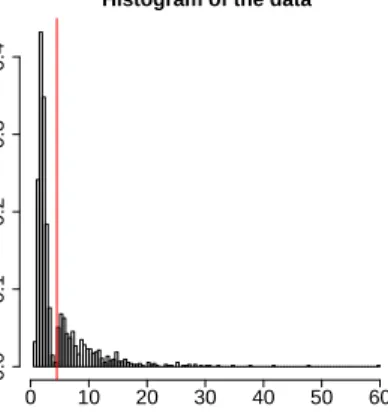
Figure 3.1 of the simulation study shows a jump between the data dis-tributed below (uniform data) and above (generalized Pareto data) the thresh-oldu. This discontinuity is represented by the red line at the point u= 5. Prior and Posterior distribution
The parameters in the model are θ = (η,σ, ξ, u˜ ). In the next paragraphs
we describe in details the priors for the parameters above, on and below the thresholdu.
Prior for parameters above the threshold
As it is not easy to express directly prior beliefs of GPD parameters, the elicitation of information is used (Coles and Powell (1996) and Coles and Tawn(1996)). Equation (2.5) is inverted and we get the 1−p quantile of the distribution,
q =u+σ˜
ξ(p
−ξ−1).
The value q corresponds to the return level associated with a return period of1/p time units.
For the generalized Pareto parameters, the prior elicitation is carried out in term of (q1, q2, q3) specifying the values of p1 > p2 > p3. Hence, we
order the parameters and q1 < q2 < q3. Coles and Tawn (1996) proposed
to work with the dierences di = qi −qi−1, i = 1,2,3. In addition, they
assume q0 =e1, where e1 is the physical lower bound of the variable. The
dierencesdi are supposed to be gamma distributed with parameters(αi, βi) fori= 1,2,3. The prior distribution of eachdiis supposed to be independent to the others. Usually we usee1 equal to zero.
The procedure to obtain the prior information is the following: rst, the median and the90% quantile (or any other) estimates for specic values of
p are required. Second, we transform the elicited parameters to obtain the equivalent gamma parameters. Notice that neither di nor qi depend on u
for i > 1. Then, we have that p(di | u) is approximated by (di | u∗) ∼
Ga(ai(u∗), bi(u∗)), whereu∗ is the prior mean for u.
In this particular case, we do not consider the location parameter, but only the scale and shape parameters. For this reason, we need only two quan-tiles. The gamma distributions for the dierences with known parameters are given by
d1 =q1 ∼Ga(a1, b1), d2=q2−q1 ∼Ga(a2, b2).
The marginal prior distribution for parametersσ˜ andξ is
π(˜σ, ξ) ∝ u+σ˜ ξ(p −ξ 1 −1) a1−1 exp −b1 u+σ˜ ξ(p −ξ 1 −1) × ˜ σ ξ(p −ξ 2 −p −ξ 1 ) a2−1 exp −b2 ˜ σ ξ(p −ξ 2 −p −ξ 1 ) × −σ˜ ξ2 n
(p1p2)−ξ(logp2−logp1)−p−2ξlogp2+p−1ξlogp1
o , wherea1, a2, b1 andb2 are hyperparameters obtained from the experts
infor-mation,σ >˜ 0 andξ ∈R.
Prior for the threshold
Dierent alternatives to dene a prior distribution foruexist. The most used are the continuous uniform prior, the discrete distribution or a truncated normal distribution with parameters (µu, σ2u), truncated from below at e1
with density π(u|µu, σu2, e1) = 1 p 2πσ2 u exp{−(u−µu)2/2σ2u} Φ[−(e1−µu)/σu] (2.11)
with µu set at some high data percentile, σ2u large enough to represent a fairly non informative prior (Behrens et al.,2004), e1 =q0 ande1< u <∞.
Prior for parameters below the threshold
According to the distribution chosen for the data below the thresholdu, the prior for the parametersη could be modied. The most suitable choice for
the prior would be a conjugate prior so that the problem has a simpler form analytically.
In this case, we assume that the data have a gamma distributionj(x|η)
with parametersη= (α, β), whereα is the shape andβ the rate parameter. It is easier to reparametrize in terms ofαandµ=α/βto have a more natural interpretation. Moreover, we assume that the shape parameter α and the mean µ are independent to simplify the computations. Both parameters have a gamma distribution,
α ∼Ga(a, b), µ∼Ga(c, d),
wherea, b, canddare known hyperparameters. Then, the joint prior density function can be written as follows,
π(η) = b a Γ(a)α a−1e−bα dc Γ(c) α β c−1 e−dα/β α β2 , wherea, b, c, d >0. Posterior inference
We take the likelihood dened in equation (2.10) and the prior distributions given in the previous paragraphs to compute the posterior distribution given by applying Bayes Theorem. As the calculations are too much complicated to carry out analytically, we apply the Markov Chain Monte Carlo methods, in particular the MetropolisHastings algorithm.
Simulation Study
In order to check the theoretical properties of measures of surprise, simula-tions are performed. In particular, we consider two cases, the prior predic-tive p-values (1.7) and the posterior predictive p-values (1.9). After that, we compare the results with two of the approaches explained in Section2.3: the parameter stability plot (see Section 2.3.1) and the mean residual life plot (see Section2.3.2).
Firstly, we look at the posterior predictive measures of surprise consid-ering three dierent samples and after that we get on to the prior predictive measures of surprise.
3.1 Posterior Predictive p-values
Considering the posterior predictive p-values dened in (1.8), m(x|xobs) =
Z
f(x|θ)π(θ|xobs)dθ,
we notice thatm(x|xobs) could be approximated by
m(x|xobs)≈ 1 N N X i=1 f(x|θ(i)), θ(i)∼π(θ |xobs). (3.1)
Then, for the parameter θ = (˜σ, ξ) of a generalized Pareto distribution,
the likelihood of a set of independent observations x= (x1, . . . , xn) can be
written as f(x|θ) = n Y i=1 f(xi|θ), (3.2)
where f(xi|θ) = ( 1 ˜ σ 1 +ξ xi−u ˜ σ −1/ξ−1 , ifξ 6= 0, 1 ˜ σexp − xi−u ˜ σ , ifξ = 0, xi > u.
In order to compute the measure of surprise (3.1), the MetropolisHastings algorithm is implemented to draw the posterior distribution. Usually to simplify the calculations of the likelihood-ratio in the MCMC algorithm, computation is performed on the log-scale (i.e. dierence of log likelihoods). This avoids evaluations of the likelihood being numerically rounded to zero. However, in evaluating (3.1) the likelihood must be evaluated on its nat-ural scale, and so is rounded accordingly to0. It is dicult to get round this
by using log likelihood computations as
log Z f(x|θ)π(θ|xobs)dθ 6 = Z logf(x|θ)π(θ|xobs)dθ
or any other computation withlogf(x|θ).
For this reason, the likelihood dened in equation (3.2) as the product of thef(xi |θ)is replaced by the mean of thef(xi|θ)so that higher likelihood values will produce a higher mean of the densities and then the surprise is more evident, f(x|θ)≈ 1 n n X i=1 f(xi |θ). (3.3)
While this approach is non-standard, this approximation gives credible re-sults and we can see them in the simulation studies. Unfortunately, no information has been found on how to compute these marginal likelihoods numerically in the literature and to support this choice. Only algebraic computations could have been found in certain circumstances.
In addition, the prior distribution is given by the Jerey's prior ( Castel-lanos and Cabras,2007),
π(θ) = 1 ˜ σ 1 1 +ξ 1 √ 1 + 2ξ σ >˜ 0, ξ >−0.5. (3.4) The procedure to approximate the integral consists of several steps. Firstly, the MetropolisHastings algorithm produces a chain of values of
θ. These parameter values come from the posterior distributionf(x|θ)
us-ing the MetropolisHastus-ings algorithm. The prior ofθ is the Jerey's prior
generalized Pareto distribution of each observation with scale parameter σ˜
and shape parameterξ. The proposal densities forσ˜ and ξ are a log-normal density distribution and a normal density distribution, respectively.
In order to generate the sample, R= 10000 iterations have been carried
out, where a burn in period of 1000 has been cut o. Furthermore, we
consider for the analysis the chains consisting in every 10−th observation.
These values are used to evaluate the distribution f(x | θ) and calculate
approximativelym(x|xobs). Finally, the probability
Prm(·|xobs){m(X |xobs)< m(xobs |xobs)}
is estimated by counting the number of times thatm(X |xobs)is less than
m(xobs |xobs)divided by the total number of simulations. Then, the
poste-rior predictive p-values can be written as
ppost= Pr{T(X)≥T(xobs)|xobs},
whereT(X) =m(X |xobs). The same study is carried out for three datasets
which are created with dierent changepoints. Two samples are generated with a known changepoint location and the third one does not have a change-point. Concerning the datasets with a changepoint, we have either some uni-form or gamma data generated below it and some generalized Pareto data generated above it. The last dataset has a generalized Pareto distribution. The purpose of looking at these dierent datasets is the detection of the known changepoint, if it exists by using measures of surprise.
3.1.1 Uniform and Generalized Pareto Data
First of all we generate two dierent datasets. The rst sample has a gener-alized Pareto distribution with parametersσ˜ equal to1,ξequal to0.2andu equal to5. Its size is n= 500. The second sample (n= 500) has a uniform
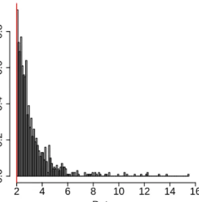
distribution on the interval [0,5]. The histogram of the complete dataset
(generalized Pareto and uniform data) is represented in Figure3.1; the red line represents the threshold u= 5.
Before starting to compute the measures of surprise, we look at dierent plots. Figure 3.2illustrates the traces of the sampled values of the param-etersσˆ˜ and ξˆestimated by MetropolisHastings algorithm. The trace plots
represent the behaviour of the parameters at each iteration for the new chain. The posterior means (red line in Figure3.2) and their95% central
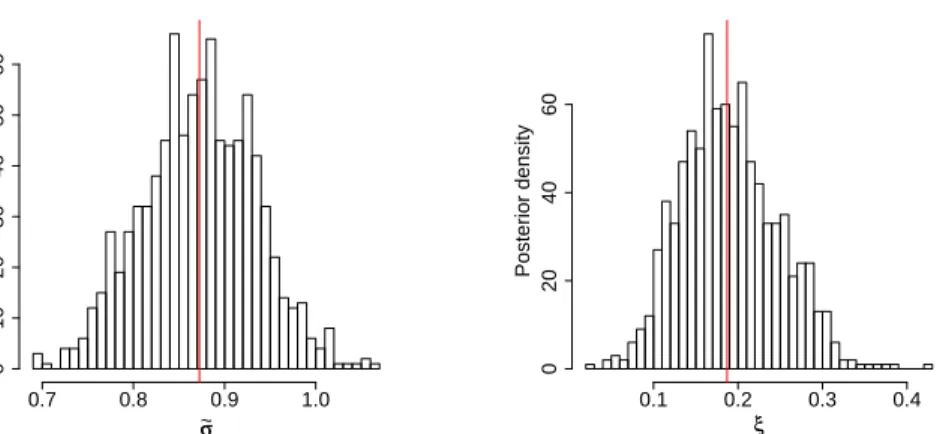
credibil-ity intervals are displayed in Table 3.1. The marginal posterior densities are analysed too. Figure 3.3shows the marginal posterior densities of each
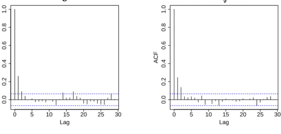
parameter and the red lines correspond to the posterior mean. Finally, the correlogram of both parameters is displayed in Figure3.4. This graph indi-cates that the chain has a stationary distribution and the observations are independent. For lags bigger than2the observed ACFs correspond to white
noise.
Histogram of the data
Data Density 0 2 4 6 8 10 12 14 0.0 0.1 0.2 0.3 0.4 0.5
Figure 3.1: Histogram of the complete dataset. Data below the threshold u= 5(red line) correspond to uniform data on the interval[0,5]. Data above
the threshold u = 5 (red line) have a generalized Pareto distribution with
parametersσ˜= 1 and ξ= 0.2.
Mean 2.5% quantile 97.5% quantile ˜
σ 0.87 0.75 0.99
ξ 0.19 0.09 0.30
Table 3.1: Estimates of the parameters and their 95% central credibility
0 200 400 600 800 0.7 0.8 0.9 1.0 σσ ~ Iterations 0 200 400 600 800 0.1 0.2 0.3 0.4 ξξ Iterations
Figure 3.2: Trace plots of the parametersσˆ˜ andξˆestimated by Metropolis
Hastings algorithm (10000 iterations have been carried out, a burn in period of length 1000 has been cut o and one every10-th observation is considered).
The red lines correspond to the posterior means for the sampled values σ˜
andξ. σσ ~ Posterior density 0.7 0.8 0.9 1.0 0 10 20 30 40 50 60 ξξ Posterior density 0.1 0.2 0.3 0.4 0 20 40 60
Figure 3.3: Marginal posterior density plots of the parameters ˆ˜σ andξˆ
esti-mated by MetropolisHastings algorithm (10000 iterations have been carried out, a burn in period of length 1000 has been cut o and one every 10-th
0 5 10 15 20 25 30 0.0 0.2 0.4 0.6 0.8 1.0 Lag ACF σσ ~ 0 5 10 15 20 25 30 0.0 0.2 0.4 0.6 0.8 1.0 Lag ACF ξξ
Figure 3.4: ACFs for the parameters σˆ˜ and ξˆ estimated by Metropolis
Hastings algorithm (10000 iterations have been carried out, a burn in period of length 1000 has been cut o and one every10-th observation is considered).
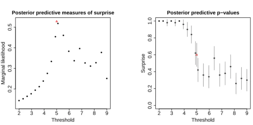
Further on, we analyse the measures of surprise and posterior predictive p-values for the thresholds from 2 to 9. Figure 3.5 shows the posterior
predictive measures of surprise (left panel) and the posterior predictive p-values (right panel) for each threshold, where the vertical lines correspond to the 95% central credibility intervals. The true threshold (i.e u = 5) is
● ● ● ● ● ● ● ● ● ● ● ● ● ● ● ● ● ● ● ● 2 3 4 5 6 7 8 9 0.2 0.3 0.4 0.5
Posterior predictive measures of surprise
Threshold Marginal likelihood ●● ●●●● ● ● ● ● ● ● ● ● ● ● ● ● ● ● 2 3 4 5 6 7 8 9 0.0 0.2 0.4 0.6 0.8 1.0
Posterior predictive p−values
Threshold
Surprise
Figure 3.5: Plot of the measures of surprisem(x|xobs) (left panel) and of
the posterior predictive p-values with their95% central credibility intervals
(right panel) for the dierent thresholds u from 2 to 9 estimated by using
the approximation given in equation (3.1). The red triangle corresponds to the proper thresholdu= 5.
Both graphs indicate that the data below the true threshold do not have a generalized Pareto distribution, that is there is evidence of surprise. The left plot shows the marginal likelihoods which increase from very small values, for a threshold far away from u = 5, to the highest value of m(x|xobs) = 0.53 at u equal to5. Then the marginal likelihood starts again to decrease.
The way, how the estimated marginal likelihoods change, aects the results concerning the p-values as its graph indicates it. In fact, the right plot shows the p-values estimated around1below the true threshold and this means that
the probability to have surprise is very high and therefore the model does not t appropriately. The reason why the p-values are very big is due to the fact that having very small marginal likelihoods, the probability to obtain larger values of the marginal likelihoods, which are obtained from the simulated dataset, than the marginal likelihood of the dataset is slight. Thus, the probability to have surprise is very high. On the other hand, small p-values indicate a slight surprise, that is the generalized Pareto model ts appropriately to the data. Furthermore, in the p-values plot we notice that the probability jump from values around1to 0.6for a threshold chosen just
below the true one (i.e. u= 4.9). We remark that the dataset considering the
threshold at4.9 has just ten observations more than the dataset generated
only from the generalized Pareto distribution. Then this jump of about 0.4
the suitable changepoint both graphs are necessary for the analysis.
Other tools to estimate the threshold are explained in Section 2and we exploit two of them to check the goodness of the model.
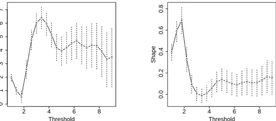
First of all, we look at the threshold selection by using parameter stability (see Section2.3.1) which consists in plotting the tted GPD parameters at dierent thresholds in order to detect a good threshold for the dataset.
Figure3.6shows the estimated values of the scale and shape parameters at each threshold from2to9. In addition, the vertical broken lines represent
the 95% central credibility intervals. Both the left and the right panels
indicate that the parameters are not stable below the threshold u = 5and
for u bigger than5 the bands cover horizontal lines, suggesting stability. A
similar result is not surprising as below the threshold u = 5 the data are
uniform distributed.
Another approach to estimate the threshold u of a dataset is the use of the mean residual life plot which has been explained in Section2.3.2. Figure
3.7illustrates the mean residual life plots for every threshold (left panel) and for the thresholds chosen for the previous studies (from2 to 9). Looking at
the left plot, we observe a slight linearity of the mean exceedance fromu= 5.
This means that the GPD distribution does not t appropriately before the true threshold. This linearity is shown more clearly in the right panel.
2 3 4 5 6 7 8 9 −5 0 5 10 15 Threshold Modified Scale ●● ● ●● ● ● ● ● ●● ● ●● ● ●● ● ● ● ● 2 3 4 5 6 7 8 9 −1.0 −0.5 0.0 0.5 Threshold Shape ● ● ●● ● ●● ● ● ● ● ● ● ●● ● ●● ● ● ●
Figure 3.6: Parameter stability plots of σˆ˜ (left panel) and ξˆ(right panel)
against the thresholds. The vertical broken lines correspond to the 95%
0 2 4 6 8 10 12 14 0 1 2 3 4
Mean Excess Plot
Threshold Mean Excess 2 3 4 5 6 7 8 9 1 2 3 4
Mean Excess Plot
Threshold
Mean Excess
Figure 3.7: Mean residual life plot for every threshold (left panel) and mean residual life plot for the thresholds from 2 to 9 (right panel). The blue
lines correspond to the 95% central credibility intervals and the red line
corresponds to the thresholdu= 5.
Once more, this result is coherent with the hypothesis considering that only the data above the threshold u = 5 have a generalized Pareto
distri-bution. Furthermore, in the left panel we observe that for a big threshold (i.e. u >9) the dataset becomes very small and thus the generalized Pareto
model does not t any more very well. In fact, there is a decreasing tendency of the mean exceedance instead of keeping a constant value.
3.1.2 Gamma and Generalized Pareto Data
A second simulation study is carried out on a sample generated by gamma and generalized Pareto data. The rst sample has a generalized Pareto distribution with parameters˜σ equal to5,ξ equal to0.1and uequal to4.5.
Its size isn= 500. The second sample has a gamma distribution with shape
parameter equal to10 and rate parameter equal to5. We take into account
only the values which are less or equal than 4.5. Figure 3.8 represents the
histogram of the complete dataset (gamma and generalized Pareto data) and the vertical red line corresponds to the changepoint (u = 4.5). The
histogram let suggest that the data appear to come from a single continuous distribution with a bit of data removed at around uequal to 4.5.
Histogram of the data Data Density 0 10 20 30 40 50 60 0.0 0.1 0.2 0.3 0.4
Figure 3.8: Histogram of the complete dataset. Data below the threshold u = 4.5 (red line) correspond to gamma data with shape parameter equal
to 10 and rate parameter equal to 5. Data above the threshold u = 4.5
(red line) have a generalized Pareto distribution with parametersσ˜ = 5and
ξ= 0.1.
A similar analysis about the outputs (posterior densities of the param-eters) of the MetropolisHastings algorithm is carried out: the marginal posterior density plots, the trace plots and the independence of the chain are studied before looking at the measures of surprise and their p-values.
Figure 3.9 shows the posterior marginal likelihoods (left panel) and the posterior predictive p-values with their95%central credibility intervals (right
panel). These graphs highlight some interesting but at the same time un-expected results. The behaviour of both the marginal likelihoods and their p-values for the thresholds between 1 and 3 is not regular. First of all,
the marginal likelihoods increase untilu equal to1.76 and after that it
de-creases until becoming innitesimal for u equal to 3.27. Respectively, the
p-values plot shows that for the highest marginal likelihood (at u = 1.76),
the surprise to have a generalized Pareto model is very small. After that it increases until1 (foru equal to 3.64).
No surprise means that the p-values is equal to zero, that is every dataset generated during the simulation is less likely than the observed one. Fur-thermore, as the observed marginal likelihood is very small, the probability to obtain bigger marginal likelihoods for the generated dataset is extremely dicult and then the surprise is estimated around zero.
● ● ● ● ● ● ●● ● ● ● ● ● ● ● ● ● ● ● ● 2 4 6 8 0.10 0.15 0.20
Posterior predictive measures of surprise
Threshold Marginal likelihood ● ● ● ● ● ● ●● ● ● ● ● ● ● ● ● ● ● ● ● 2 4 6 8 0.0 0.2 0.4 0.6 0.8 1.0
Posterior predictive p−values
Threshold
Surprise
Figure 3.9: Plot of the measures of surprisem(x|xobs) (left panel) and of
the posterior predictive p-values with their95% central credibility intervals
(right panel) for the dierent thresholds u from 1 to 9 estimated by using
the approximation given in equation (3.1). The red triangle corresponds to the proper thresholdu= 4.5.
Observing the histogram (see Figure3.8) we notice a drop just before the true threshold. Two dierent interpretations of this plot can be possible: the rst one is that the data come from two separate datasets and the second one it that there is a unique dataset coming from a continuous distribution with some data missing. As shown in Figure 3.9 this duel interpretation aects the results of the posterior marginal likelihoods and the posterior predictive p-values. In fact, for low threshold (i.e. u <3), when data are generated to
estimate the p-values, consistently with the second interpretation, the drop is not taken into account because we have a lot of data and they seem to have a generalized Pareto distribution. Thus the surprise will be small for very low threshold values. On the other hand, when the threshold u is chosen just around 4 (or possibly <1.76), the data will not be generalized Pareto
distributed. Therefore instead of having a small surprise we have a surprise which increases as we move below the thresholdu = 4 (or u = 1.76). This
occurs in the rst case (u < 1.76) because we have too much gamma data
than generalized Pareto data and in the second case (3< u <4) because of
the presence of the drop.
Then for the analysis we cannot consider the results for u less than 3.
The reason why we cannot consider the thresholdu equal to1.76as credible
is because if data are really generalized Pareto distributed, they should be GPD for all thresholds above u. This is not true for u = 1.76 but it is
true for u = 4.5. Therefore, analysing both graphs we can conclude that
approximately the right threshold is around4.5.
2 4 6 8 0 1 2 3 4 5 6 7 Threshold Modified Scale ● ● ● ● ● ● ● ● ● ● ● ● ● ● ● ● ● ● ● ● ● 2 4 6 8 0.0 0.2 0.4 0.6 0.8 Threshold Shape ● ● ● ● ● ● ● ● ● ● ●● ● ●● ● ●● ● ●●
Figure 3.10: Parameter stability plots of σˆ˜ (left panel) and ξˆ(right panel)
against the thresholds. The vertical broken lines correspond to the 95%
central credibility intervals.
0 10 20 30 40 50 60
0
5
10
15
Mean Excess Plot
Threshold Mean Excess 2 4 6 8 3 4 5 6 7
Mean Excess Plot
Threshold
Mean Excess
Figure 3.11: Mean residual life plot for every threshold (left panel) and mean residual life plot for the thresholds from 1 to 9 (right panel). The
blue lines correspond to the95%central credibility intervals and the red line
corresponds to the thresholdu= 4.5.
Looking at the outcomes displayed in the parameter stability plots (see Figure 3.10) and the mean residual life plots (see Figure 3.11), we have
![Figure 3.1: Histogram of the complete dataset. Data below the threshold u = 5 (red line) correspond to uniform data on the interval [0, 5]](https://thumb-us.123doks.com/thumbv2/123dok_us/11095633.2996834/35.918.363.555.354.551/figure-histogram-complete-dataset-threshold-correspond-uniform-interval.webp)