Gunjan Chandra
IMPACTS OF DATA SYNTHESIS: A METRIC FOR
QUANTIFIABLE DATA STANDARDS AND
PERFORMANCES
Master’s Thesis
Degree Programme in Computer Science and Engineering
June 2020
ABSTRACT
Publicly shared data could unfold a wide range of innovative pedagogical and learning techniques. In the case of healthcare, open data could save lives. Consolidating medical data with lifestyle information can support possibilities for further development of current approaches towards medical diagnoses and treatments. It is critical to note that healthcare data contains sensitive information about patients and therefore, could lead to harmful consequences if such details reach the wrong hands. The use of the concept of data anonymisation for reducing the risk of disclosure to share data publicly is the standard practice. However, current data anonymisation techniques have failed multiple times in the past. The goal of this study is to evaluate the performance of an emerging practice for data sharing, by utilising a tool for data synthesis, termedSynthpop. The synthetic data is generated by executing the multiple imputation methods, although differently. This study describes and analysesSynthpopby establishing the data standards and measuring the impacts of the data synthesis process based on the utilities and quality of information contained in the data. The analyses reveal that synthetic data simulates original data by adequately preserving the utilities and quality of the information content.
Keywords: Synthpop, Data Sharing, Privacy, Data Anonymisation, Machine Learning, Data Utility, Entropy, Information, Data Quality, Type 1 Diabetes, Human Activity Recognition.
ABSTRACT
TABLE OF CONTENTS FOREWORD
LIST OF ABBREVIATIONS AND SYMBOLS
1. INTRODUCTION... 7
2. RELATED WORK... 9
2.1. Benefits of Open Healthcare Data Sets ... 9
2.2. Importance of the Subject’s Privacy ... 10
2.3. Data Anonymisation ... 10
3. METHODOLOGY... 14
3.1. Synthpop... 14
3.1.1. Basic Functionality... 14
3.1.2. Methods for Synthesis ... 15
3.1.3. Controlling the Sequence and Prediction... 17
3.1.4. Handling Data with Restricted or Missing Values ... 18
3.2. Utility Measures of Data ... 18
3.2.1. General Utility Measures ... 19
3.2.2. Specific Utility Measures ... 20
3.3. Quality of Information Content... 25
3.3.1. Entropy... 25
3.3.2. Mutual Information ... 26
3.4. Data Sets... 27
3.4.1. DIPP Data Set... 27
3.4.2. HAR Using Smartphone Data Set... 28
4. EXPERIMENTS AND RESULTS ... 33
4.1. DIPP Data Set ... 33
4.1.1. Specific Utility ... 34
4.1.2. General Utility ... 39
4.1.3. Quality of Information Content ... 43
4.1.4. Outlines... 44
4.2. HAR Using Smartphone Data Set ... 45
4.2.1. Specific Utility ... 45
4.2.2. General Utility ... 52
4.2.3. Quality of Information Content ... 54
4.2.4. Outlines... 55
5. DISCUSSION ... 57
5.1. Principal Discoveries ... 57
5.1.1. DIPP Data Set... 57
5.1.2. HAR Data Set ... 58
5.2. Synopsis and Future Work... 60
6. CONCLUSION ... 61
This study was conducted under and supported by the Biomimetics and Intelligent Systems Group (BISG) of the Computer Science and Engineering Department of the Faculty of Information Technology and Electrical Engineering at the University of Oulu, Oulu, Finland.
I want to express my most profound appreciation to my thesis supervisor Dr Pekka Siirtola and reviewer Dr Satu Tamminen, for their constructive feedback, patience, and valued guidance. Special thanks to Dr Eija Ferreira for her insightful suggestions regarding the growth and completion of the study. I would further like to extend my gratitude to Dr Ian Oliver and his team for presenting me with the grounds concerning the Mutual Information analyses. Additionally, I am indebted to MSc Oana M. Stoicescu for providing me with the assistance and means to complete this work. Finally, appreciation to Johan Estiévenart for supporting me throughout the process.
Oulu, June 16th, 2020
Abbreviations
ADL Activities of Daily Living ALE Accumulated Local Effects ANN Artificial Neural Networks
CART Classification And Regression Tree
DIPP Type 1 Diabetes Prediction and Prevention EHR Electronic Health Record
FFT Fast Fourier Transform FI Feature Importance
FN False Negative
FP False Positive
GADA Glutamic acid decarboxylase GBM Gradient Boosted Machine
GDPR General Data Protection Regulation HAR Human Activity Recognition HCC Human-Centered Computing
HIPAA Health Insurance Portability and Accountability Act IA2A Protein tyrosine phosphate autoantibody
IAA Antibodies of insulin
IBM International Business Machines IDC International Data Corporation k-NN k-Nearest Neighbour
LDA Linear Discriminant Analysis MI Mutual Information
NN Neural Networks
PPMCC Pearson product-moment correlation coefficient
SYLLS Synthetic Data Estimation for UK Longitudinal Studies T1D Type 1 Diabetes
TN True Negative
TP True Positive
t-SNE T-distributed Stochastic Neighbor Embedding UMAP Uniform Manifold Approximation and Projection
ZB Zettabytes
Symbols
C⇤ Comparison function
C(y|k) Cost of classifying an observation asywhen its true class is k
D Original Data set
D⇤ Kolmogorov-Smirnov statistic
ˆ
F empirical distribution
G Tangent sigmoid transfer function Ho Null hypothesis
L Loss function
M Number of iterations P,p Probability of occurrence P(k) Prior probability of classk
ˆ
P(k|x) Posterior probabilty of classkfor observationx R Correlation coefficients
Si Synthetic data sets
W(l) Weights matrices
X,Y Random variables
argmin Argument of the maximum b(l) Bias vectors
dist Distance
exp Exponential
i Target class vector
j Weak learner
k Positive integer
log Logarithmic
n Matrix of net input (column) vectors s Soft max transfer function
sum Summation
sup Supremum function
t Vector of tests
x Matrix (nxp) of original covariates xp Matrix (kxp) of synthesised covariates y Original data vector of lengthn
ˆ
y Predicted classification
P
Summation
↵ Threshold value for level of significance
im Residuals
" Privacy loss parameter
⇢ Population correlation coefficient
Standard deviation Di-gamma function
1. INTRODUCTION
In today’s digital era, with the exponential growth in the quantity and quality of data collection methods, over 2.5 Quintilian bytes of data are created every single day [1], and International Data Corporation (IDC) predicts that it is only going to grow from there, from 33 Zettabytes (ZB) in 2018 to 175 ZB by 2025 [2]. By 2020, there will be 44 ZB of data, suggesting 40 times more bytes of data than there are stars in the observable universe [3]. Regardless of the size, data helps us in solving problems, making better decisions, maintaining performances, and improving existing processes [4]. Despite the benefits, as of 2013, only 0.5% of the total data was analysed [5].
To keep up with the speed of data generation, data collectors could make the data publicly available and target more analysts around the globe. Open data sets have many other advantages as well, ranging from consolidating different data sets for finding new knowledge to verify previously made findings. Currently, to fulfil these requirements, researchers duplicate the data collection, which is an unnecessary use of resources. Private data also restrict scholars to share in-depth knowledge of the topic and impose a limitation on communication. Transparency in the research community is not only going to help in the advancement of the technology but will also facilitate better opportunities for innovations and solving current problems.
However, making the data set publicly available increases the risk of disclosure. In the survey done by Morey T., Forbath T., and Schoop A., more than 72% of United States citizens reported being worried about sharing personal information online [6]. If data reaches the wrong hands, sensitive information can be exploited for blackmailing, mass surveillance, social engineering, or identity theft [7]. All these risks obtrude data collectors and researchers from sharing the data and opt for proprietary data policy. Not alone researchers but also students suffer from this; for example, teaching data analysis with medical data such as Electronic Healthcare Record (EHR) is significantly restrained by laws protecting the patients’ privacy in many countries [8]. Notwithstanding the benefits, the limitations imposed by these laws hinder innovation and limit educational opportunities.
Sensitive data as defined by General Data Protection Regulation (GDPR) can be any data that reveals the racial or ethnic origin of a person, political opinions, religious or philosophical beliefs, trade union membership, genetic data, or use biometric data to uniquely identify a person and data concerning health or a person’s sex life or sexual orientation [9]. After GDPR came into force on May 25th 2018, the collection, sharing, and processing of data has become more secure than ever but, at the same time, data acquisition has become more difficult for researchers. Determining whether a subjects’ consent is required for secondary data use in research, and which forms to be filled, further slows down the process.
In the healthcare sector, medical data either collected as part of clinical research or recorded during clinical practice is considered as confidential and needs to be pseudonymised or anonymised before leaving the hospital [10]. Traditional pseudonymisation and anonymisation techniques consist of the removal of identities such as names, addresses, and national identity numbers. This method solves the issue of direct identification, but a person can still be re-identified when data is re-linked to other data sets, and the risk in the reduction of k-anonymity can be expected [11, 12]. To further reduce the risk of re-identification, data scientists use data aggregation
techniques and induce random noise to the data, which leads to distortion of the relationship between variables in the data set [11]. Having a data set with distorted relationships between variables can be misleading [13]. As the correlation between the features changes, the risk that correlation is interpreted as causation increases and can lead to misconceptions [14].
Another problem could come from a perspective of different expertise as one researcher has the data but does not have machine learning knowledge, for example. Not being able to share data, in this case, could hinder data exploration. The generation of the synthetic data set, which preserves the statistical properties of the original data set and, simultaneously, ensures the patient’s privacy, will be the fittest case in the current scenario to share data. In this study, a data synthesis tool, an R package termed Synthpop will be explored and examined while underlining the statistical properties, machine learning applicability, and quality of information contained in the data set. The primary objective will be to question the performance of the synthesis tool by evaluating the impact of data synthesis procedure; Over two different data sets for comprehensiveness evaluation. The first data set is the Finnish Type 1 Diabetes Prediction and Prevention (DIPP) study database [15], pre-processed by M.Sc. Oana Maria Stoicescu and second is the Human Activity Recognition (HAR) data set from the University of California Irvine machine learning repository [16]. Impacts of data synthesis will be measured based on the general and specific utility, and quality of information of the synthetic data set compared to the original data set. General utility measures will evaluate the difference in the statistical properties of the data sets, and specific utility measure will focus on the performance of the fitted models over different data sets (synthetic and original). One null and one alternative hypothesis will be defined, evaluating the difference in the results of utility measures. TheSynthpop will succeed in a performed test if results fail to reject the null hypothesis, which states that the two data sets (synthetic and original) have at most a statistically non-significant difference. Moreover, the study will be finalised via evaluating from an information-theoretic point of view, by analysing entropy and mutual information within the data sets or in comparison to measure the quality of information contained in the data set.
2. RELATED WORK
2.1. Benefits of Open Healthcare Data Sets
The maintenance of data obtained as a part of the clinical analysis has evolved. Initially, medical data was generated and maintained by health care professionals in the form of several EHR. Nowadays, most countries possess a centralised EHR system to accommodate the availability and completeness of the data. The purpose of centralised EHR is to hold detailed information about the patient’s medical archives in one place. These centralised EHR can later be combined with other data sets to help medical professionals administer the best possible treatment with knowledge gained from data by using next-generation technologies. Despite the benefits, few considerable obstacles prevail in the process of exploring and achieving this goal [17]. Some are associated with the content and structure of the modern healthcare database; others regard the complications and expense of producing and sustaining comprehensive databases.
On that account, within the fastest-growing field of science, the collaboration between medical professionals is continuously growing with other doctors, healthcare providers, drug providing companies, and data scientists to study and sustain the data. Trade of knowledge and data is part of the ubiquitous global movement [18]. Furthermore, it is advancing science along with the transformation of healthcare systems and how we make decisions.
In healthcare, open data can save lives by enabling new data-driven technologies, including artificially intelligent systems, and potentially transform medicine. Precision medicine [19] is an emerging model-based technique for patient care that weighs the peculiar variability in genes, environment, and lifestyle to provide treatment tailored to individual characteristics of each patient. Precision medicine involves the amalgamation of both clinical and lifestyle information of patients to provide precise intervention.
An approach such as precision medicine relies on the varieties and sources of data. The performance of the predictive model for acquainting clinical practice depends on the size and diversity of data. Lack of cohort diversity in data can lead to bias and inequity. For example, International Business Machines (IBM) Watson revealed a bias towards treatment provided at the hospital from where originally data was collected [20]. Hence, a practical advantage of open data is not merely that we can use an individual database more extensively; it is the ability to leverage and consolidate with other databases. The study reveals that machine learning models perform far better with more diverse longitudinal data sets [21].
However, those rich veins of data are too often locked away. There are several reasons why every data set is not publicly available. Most often, data collectors do not get the recognition of their investment in data collection; hence the desire to be the first to explore and utilise the data before they sell or distribute it to others. Nevertheless, one being the most important reason is the privacy of the subjects.
2.2. Importance of the Subject’s Privacy
After coming across the benefits of open data, mainly governments are spearheading the concept of open databases over the last decade. With open database comes the risk of disclosure and can lead to many harmful consequences. Disclosure risk gets higher with a better privacy attack. Privacy attack is the method of identifying a subject’s identity within the data set or by combining multiple databases. Once a subject is identified, the knowledge can be used for blackmailing, mass surveillance, social engineering, or identity theft [7].
Medical history, which includes information about the sexually transmitted disease, substance abuse, psychiatric treatment, or elective abortion, are sensitive pieces of information about a person, and the person may not want to reveal this information to anyone except specialists. A person can also wish to not reveal any private information for no particular reason because they feel invaded and find the entire system distasteful [22].
As per law in most countries, data sharing is possible with the given consent from the data owner, providing that the person’s identity will remain anonymous. In order to continue exercising data sharing and collection, many different data anonymisation techniques are brought into play.
2.3. Data Anonymisation
Those who wish to release a version of data publicly opt for traditional data anonymisation techniques. Irreversibly altering the data with the intention of privacy assurance is a method called data anonymisation [10]. Anonymisation can be done by either encrypting or removing personally identifiable information. Data is said to be anonymous if the subject’s identity can no longer be identified directly or indirectly.
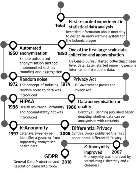
Data anonymisation approaches have evolved, developed, and adapted to our need multiple times in past. Figure 1 provides a brief history of data anonymisation and the starting point of knowledge discovery. Around 1850, when the US Federal Bureau of Statistics (Census Bureau) started receiving questions about privacy, as a protection measure, the Census Bureau began to remove personal information from publicly available census data. Census Bureau became one of the first to adopt data anonymisation concept by removing explicit identifiers such as name, address, and national identity numbers as this information can be misused, abused, or not comply with the agreement of the data sharing policy mentioned during data collection. Herman Hollerith, famously recognised for founding IBM, invented the tabulating machine for Census Bureau. Later in 1950, Census Bureau became the first to use the tabulating machine to assist in summarising information. In early 1960, as the US government decided to set up the National Data Centre to improve state information system, which the public viewed as contradicting with constitutional rights. The same debate was repeated in Europe—directing the German state of Hesse to introduce the Hessian Data Protection Act in 1970 [23] and the US to pass the Privacy act in 1974 [24].
Figure 1. History of data anonymisation
In 1972, a paper proposing the concept of inducing noise to data was published [25]. Later in 1980, researcher Dorothy E. Denning published a paper showing concern whether data can be anonymised with certainty as her analysis showed that "noise" can often be removed by averaging responses for carefully selected query sets [26]. For additional disclosure protection, data aggregation and sampling, alongside with inducing random noise to sensitive variables were standard practices before sharing data. These practices make it challenging to identify an individual, yet the risk of producing data with distorted relationships between variables increases [27].
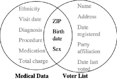
Figure 2. Linking data for re-identification
For almost 15 years until the Health Insurance Portability and Accountability Act (HIPAA) was enacted, the entire computer science community had lost interest in data anonymisation. Soon after in 1997, Latanya Sweeney succeeded to re-identify then Massachusetts Governor from supposedly anonymised health data and presented the concept ofk-anonymity [28]. Figure 2 represents an example of re-identification through data linking [11]. Later in 2002, L. Sweeney also provided the k-anonymity model to overcome the shortcomings of earlier anonymisation techniques [11]. Anonymised data can occupy a quality such as k-anonymity [11], and k-anonymity can be used as one of the analyses for the level of anonymity. If the information for each individual contained in the anonymous data cannot be distinguished from at least k-1individuals whose information also appears in the anonymous data, the data set is consideredk-anonymity protected [11]—assuming that the anonymised data remains practically useful. Soon after, the k-anonymity model was enhanced by introducing
`-diversity andt-closeness to the model [29, 30].
In 2006, a paper about differential privacy was published stating that privacy can be preserved by calibrating the standard deviation of the noise according to the sensitivity of function f [31]. Differential privacy uses the parameter " to determine the degree
of privacy which is inversely proportional to the value of". In other words, for better
protection, the value for"must remain low. After eight years, in 2014, the theory was
put into practice by Google as they began to collect differential private user statistics in Chrome [32]. Two years later, Apple started using differential privacy on user data for iPhones [33].
Since a data set with a low " value can only be queried a few times, questions
of utility versus privacy started to emerge. For example, data set with " value less
than one can only be queried around a few 10s of queries in total, after that access to the data is no longer authorised as the privacy can not be assured. Therefore, in order to access the data set more often"needs to be large, which leads to sacrifice in
the data protection. Despite the efforts, there is a growing consensus that traditional anonymisation techniques have proven to fail multiple times in the past [11, 34, 35].
In 2018, The General Data Protection Regulation (GDPR) came into force, allowing the data subjects to decide on the usage and disclosure of their data. Furthermore,
GDPR holds data collectors responsible for evaluating proposed research before sharing the data. This ensures adequate provision to protect the subject’s privacy and maintain the confidentiality of the subjects in data set [36]. After understanding the complexity of today’s digital databases and how privacy attacks can be personalised and can benefit by consolidating other databases to identify individuals; many researchers, scientist, and mathematicians collaboratively are taking up the task to build and advance data anonymisation procedures to make them suitable for current data needs. A novel tool proposing an alternative approach towards data sharing termed Synthpop [37] was utilised later in 2018. A synthesised version of highly sensitive data probing the role of ovulatory changes on sexual desire and behaviour was publicly released [38]. The data set consists of 26 thousand diary entries from women. Considering the sexual diaries are extremely sensitive and hard to anonymise completely, the data collector did not request the consent from participants to make data publicly available, but instead synthesised the data and made it publicly available for secondary data analysis. In this study, the performance ofSynthpop, that produces a synthetic version of data which is said to be anonymous, will be explored and examined by measuring the impacts of the data synthesis process.
3. METHODOLOGY
Medical data is considered to be highly sensitive and legally owned by patients in many countries. In order for data to be most useful for diagnosis, prognosis, and treatment planning, the identity of the patients must, in most cases, be relinked to the data analytic results. Usually, medical data is anonymised before leaving the hospital, but as the patient’s identity is often needed to be relinked, therefore medical data cannot be fully and irreversibly anonymised [10, 12]. Medical data requires complex pseudonymisation procedure to ensure k-anonymity, which is considered legal and is ethically acceptable [11]. Furthermore, especially for healthcare data, more sophisticated tools to measure the impact of data anonymisation are needed. In this chapter, Section 3.1 introduces the primary method of data synthesis, used as a function for data anonymisation and synthesis. Sections 3.2 and 3.3 explain various ways to measure the utilities and the quality of information contained in the generated data, respectively. Moreover, Section 3.4 describes the data sets used in the experiments to analyse the comprehensiveness of theSynthpop-generated synthetic data.
3.1. Synthpop
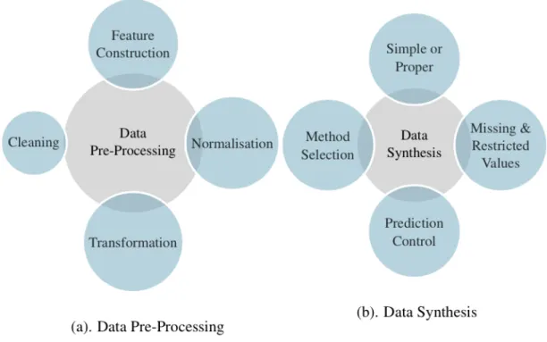
Data synthesis is a process of generating data that mimics the original data set but does not hold any disclosure records. Figure 3 represents the workflow of generating synthetic data in brief and Figure 4 gives details of sub-processes.
Raw Data Pre-ProcessingData Data
Synthesis Synthetic Data Figure 3. Workflow of generating synthetic data
The tool for data synthesis used in this research is an R package termed synthpop [37]. Thesynthpoppackage was written as a part of the Synthetic Data Estimation for UK Longitudinal Studies (SYLLS) project. Formerly to share the sensitive population-level data outside the setting where researchers were holding the original data set. Later, thesynthpoppackage was altered to makes it applicable to other data sets.
3.1.1. Basic Functionality
The method works by replacing some or all observed values by sampling from an appropriate probability distribution, conditional on the variable to be synthesised, the values from all previously synthesised columns of the original data set, and the fitted parameters of the conditional distribution (simple synthesis) or posterior predictive distribution of parameters (proper synthesis) while retaining the statistical properties of the original data set and relationships between the variables. The synthetic data can be produced simply viasyn()in a single command providing a data set, which is a data frame or matrix to be synthesised. Users can customise the synthesis of a
Figure 4. Data pre-processing and synthesis
data set according to requirement, applicability, and type of data variables for better performance of the overall system. By default, the syn() function produces one synthetic data set, but multiple data sets can be generated by setting the parametermto a coveted number. An additional parameterseedcan be used to fix the pseudo-random number generator to reproduce the same results. By default, syn() function uses simple synthesis but proper synthesis can be done by setting theproperargument to TRUE.
3.1.2. Methods for Synthesis
TheSynthpopconsists of both parametric and non-parametric methods. Table 1 lists the methods currently implemented in Synthpop. Each method generates synthetic values for each variable sequentially. Synthetic values are generated using the distribution of variable to be synthesised conditional on the distribution of previously observed synthetic and original variables called predictors. The default method of synthesis is"cart"for all variables with predictors. The method"cart"is a non-parametric method based on Classification And Regression Tree (CART); capable of handling any type of data. However, the first variable to be synthesised in the data set does not have a predictor, and it is a particular case where its values are by default generated by random sampling with replacement from original values ("sample" method). However, the user does not need to use the same method of synthesis for all variables with predictors; a user can assign different methods from the list of methods to each variable in the data set befitting the type of data. On the other hand, by setting parameter method to"parametric" assigns default parametric
methods to each variable based on their data type. Furthermore, if a user does not want to change or synthesise a variable, an empty method (" ") should be used for that variable. Finally, a new method of synthesis can be defined by writing a function named syn.newmethod() and for synthesis, specify the method parameter of syn()as"newmethod".
Table 1. Built-in synthesising methods. * Indicates default parametric methods [37].
Implementation of methods
Let y denote an original data vector of length n, xp denote a matrix (k x p) of synthesised covariates, andxdenote a matrix (nxp) of original covariates.
1) Classification tree ("syn.ctree") or Classification and regression tree ("syn.cart"):
It fits a classification or regression tree by binary recursive partitioning followed by finding a terminal node for each xp. Finally, a donor from the members of the node is randomly drawn and take that draw’s observed value as the synthetic value. The difference in"syn.ctree"and"syn.cart"is that they uses functions from different packages. "syn.ctree"usesctreefunction frompartypackage, whereas, "syn.cart" uses rpart function from rpart package. The selection of splitting variables and a stopping rule for the spitting process makes them differ amongst others. 2) Random forest("syn.rf"):
Uses Breiman’s random forest algorithm for classification and regression [39]. Furthermore, It utiliserandomForest function from therandomForestpackage. 3) Bagging("syn.bag"):
Generates synthetic data using bagging by utilising randomForest function from therandomForestpackage with number of sampled predictors equal to number of all predictors.
It is used for the synthesis of binary variables by the non-Bayesian or approximate Bayesian logistic regression model. For non-Bayesian method, it first fits a logistic regression to the original data, then calculate the predicted inverse logits for synthesised covariates. Finally, compare the inverse logits to a random (0,1) deviate and obtain synthetic values. For approximate Bayesian method (for proper synthesis), it repeats the same process as for non-Bayesian method with one additional step before computing inverse logits, drawing coefficients from normal distribution with mean and variance estimated in first step.
5) Normal Linear regression preserving the marginal distribution ("syn.normrank"):
First synthetic values of Normal deviates of rank of the values in y are generated using the spread around the fitted linear regression line of Normal deviates of rank givenx. Then synthetic Normal deviates of ranks are transformed back to get synthetic ranks which are used to assign values from y. Whereas, for proper synthesis, the regression coefficients are drawn from normal distribution with mean and variance from the fitted model.
6) Unordered polytomous regression("syn.polyreg"):
The synthetic categorical variables are generated by the polytomous regression model. First, it fits categorical response as a multinomial model, then it computes predicted categories, and finally, add appropriate noise to predictions. The algorithm uses multinom function from nnet package. Numerical variables are scaled before fitting to cover the range (0,1).
3.1.3. Controlling the Sequence and Prediction
Synthetic values of each variable are generated from a joint distribution. The joint distribution is defined in terms of a series of conditional distributions. The values are imputed sequentially from the distribution of the variable to be synthesised conditional on two distributions: 1) The distribution of all previously observed variables in the original data set, 2) The distribution of all previously synthesised variables. This sequential process is by default automated, following the order of how variables appear in the data set (left to right). However, the order can be changed or specified for each variable by listing out the indices of columns in the desired order to set parameter visit.sequence. If a user wishes not to synthesise a variable and not use it as a predictor, it should be removed from the visit.sequence. Furthermore, if a user wishes not to synthesise a variable, yet wishes to use the variable as one of the predictors for the synthesising model, then an empty (" ") method should be used while keeping the variable in visit.sequence. Note that variable/s to be synthesised later invisit.sequencecan not be used as predictor/s for variable/s which appears before it. Though, variable/s can explicitly be removed as a predictor/s for any specific variable/s by updating thepredictor.matrix. The predictor.matrix is a matrix with ones and zeros; Ones indicates that the variables should be used in the prediction model for generating synthetic values for a particular variable and zeros for otherwise.
3.1.4. Handling Data with Restricted or Missing Values
Relationship between variables can diversify significantly within a data set. Some variable can have a dependency on each other or could be tightly linked. As the goal of the synthetic data is to mimic all characteristics of the original data, these restrictions should be preserved during the data synthesis process. For example, in a medical data set, the variable containing information about the patient’s sibling’s medical history is restricted to the variable containing information whether the patient has siblings; This restriction needs to be addressed in order to get the best results out of the synthesis process. Simply when other variables determine the value for some case, the rule and corresponding values should be specified using rule and
rvaluesparameters. Furthermore, if the data set has missing values and the values
are defined with something distinct than the R missing data code NA, it should be specified incont.naparameter of thesyn()function. Missing values in categorical variables are handled as additional categories. However, missing values in continuous variables are modelled in two steps. First, an auxiliary binary variable is synthesised to model whether a value is missing or not, and if there are multiple types of missing values, an auxiliary categorical variable is created to record this. Second, a synthetic model is fitted to missing values, and synthetic values are generated for non-missing categories in the auxiliary variable. Finally, the auxiliary variable, variable with non-missing values, and zeros for remaining records are used for prediction of other variables.
3.2. Utility Measures of Data
The purpose of a synthetic data set is to resemble all the properties of the original data set. Thus, analyses made on synthetic data set should lead to the same conclusions to the analyses made on the original data set. In theory, to achieve the formally mention purpose, the model used for the synthesis process should resemble the process of the original data generation. The methods to assess the utility of the synthetic data set can be broadly divided into two approaches: general utility and specific utility [40]. General utility assesses whether synthetic data have overall similarities in the statistical properties and multivariate relationships with the original data set. Whereas, specific utility assesses the similarity of performance of a fitted model on the synthetic data to the original data. The Synthpop package provides two types of analyses for the synthetic data set based on the general and specific utility of the data set utilising the compare()function in the package. First is the relative frequency distribution, and second is the linear machine learning model’s confidence interval overlap. However, in this study, besides relative frequency distribution from the package, more rigorous analyses will be performed.
The overall utility of the synthetic data will be assessed on how adequately synthetic data succeed at all conducted utility tests. In order to succeed at a utility test, synthetic data need to resemble all the properties of the original data with at most statistically non-significant difference. For formal assessments, hypothesises will be as follows: LetDdenote an original data set, andSi denote a synthetic data set whereiindicates
denote a vector of tests which returns a statistic, and C⇤ be a comparison function which returns a p value. Finally, comparing the output ofC⇤ with↵, a threshold
value for the level of significance.
Ho :C⇤{t(D), t(Si)}>↵, for allt2[0,⌧]
Ha :C⇤{t(D), t(Si)}<↵, for anyt2[0,⌧]
The quality of the synthetic data will be estimated based on whether utility tests lead to failing to reject the null hypothesis. In order to fail to reject the null hypothesis, synthetic data must have p valuelarger or equal to ↵for all utility tests. The null
hypothesis will be rejected if synthetic data possessp valuesmaller than↵for any
utility test leading to accept the alternate hypothesis. Note that the↵is set to 0,05for
all tests.
3.2.1. General Utility Measures
Data visualisation is the presentation of data in a visual or graphical format. A visual representation of data helps data analysts to process information from data faster than from written information. Visualisation of frequency distribution can reveal a lot about the data and its properties. Four principal characteristics of the frequency distribution are [41]:
1. The measure of central tendency and location (mean, median, mode) 2. The measure of dispersion (range, variance, standard deviation) 3. The extent of symmetry/asymmetry (skewness)
4. The flatness or peakedness (kurtosis)
On the other hand, relative frequency distribution provides the fraction or proportion of times a value occurs in data sets. A side-by-side univariate distribution of each variable in the synthetic and original data set will be plotted to compare the changes in the probability distribution, which can be used to determine the likelihood of specific results to occur within a given population [37]. Furthermore, the two-sample Kolmogorov–Smirnov test will be used to evaluate whether two underlying one-dimensional probability distribution differs in two different data sets (original and synthetic data set) for each variable. Since two data sets can possess nearly identical statistical properties, yet have very different distributions. In this case, the Kolmogorov–Smirnov statistic is:
D⇤ =sup
X
(|Fˆ1(X) Fˆ2(X)|) (1)
whereFˆ1 andFˆ2 are the empirical distribution functions of the first and the second
sample, respectively [42]. Andsupis the supremum function. Moreover, the Cucconi test will be performed to evaluate whether the scale and location of the two data
set have a statistically significant difference by comparing the central tendency and variability.
Apart from visualising frequency distributions, visualisation of data points itself can help data analyst have a look at data from a different perspective. Visualisation of data directly, which has more than three dimensions is currently out of scope, but dimension reduction techniques which preserve the relationship between variables can be used as a pre-step. Uniform Manifold Approximation and Projection (UMAP) is a dimension reduction technique that can be used for visualisation similarly to T-distributed Stochastic Neighbor Embedding (t-SNE) [43], but also for general non-linear dimension reduction [44]. UMAP is constructed from Riemannian geometry and algebraic topology based theoretical framework. The result is a scalable algorithm that applies to real-world data. Despite being similar to t-SNE, it is competitive for visualisation quality and arguably preserves more of the global structure. Following the dimension reduction of the data, while preserving both global and local structures, data can be visualised in either two or three dimensions.
The bivariate Pearson product-moment correlation coefficient (PPMCC) is a parametric measure of the linear correlation between pairs of continuous variables. PPMCC produces a sample correlation coefficient, R, which measures the strength and direction of the linear relationship. The PPMCC also evaluates whether there is significant statistical evidence for a linear relationship among the same pairs of variables, represented by a population correlation coefficient, ⇢ (rho). The Pearson
correlation between variablesX andY is calculated as:
⇢(X, Y) = cov(X, Y)
x y
, (2)
where cov is the covariance of variablesX and Y, x is the standard deviation of
variable X, and y is the standard deviation of variable Y. It is beneficial to note
that a data set which does or does not have linear correlations, nevertheless, can have non-linear or complex correlations.
3.2.2. Specific Utility Measures
The specific utility of the data can be assessed by comparing the performance of the fitted synthetic and original models. In this thesis, multiple machine learning models were used as classifiers, such as Gradient Boosting Machine, Pattern Recognition Network, k-Nearest Neighbours, and Linear Discriminant Analysis. Needless to say, most of these models can also be used for regression. Different types of machine learning models were used to evaluate the generality of the primary method of synthesis "Synthpop". Moreover, the performance of the fitted model will be examined on multiple parameters for overall performance estimation.
Gradient Boosting Machine
Boosting algorithms were initially introduced by the machine learning community [45, 46, 47] for classification problems. The principle approach of the boosting algorithms is to combine several simple models iteratively, termed weak learners to
obtain a strong learner with improved predictive accuracy. A new statistical point of view for boosting was introduced to connect the boosting algorithm to the concept of loss functions [48]. Later, an extended boosting algorithm for regression termed Gradient Boosting Machine (GBM) was introduced [49]. The GBM is similar to a numerical optimisation algorithm that aims to find an additive model that minimise the loss function. Thus, GBM is a classification and regression forward learning ensemble technique, which generates a prediction model in the form of an ensemble of weak prediction models, typically decision trees that best reduces the loss function. This study follows the GBM algorithm implemented in H2O package in R [50], which follows the algorithm specified by Hastie et al. [51 p. 359-360]. The functionf0(x)is
estimated by minimising loss functionLover the training data set. Algorithm 1. Gradient Boosting Machine
1 Initializef0(x) = argmin PNi=1L(yi, ) 2 Form= 1toM:
3 (a) Fori= 1,2,. . . ,N compute
4
rim=
@L(yi, f(xi))
@f(xi) f=fm 1
5 (b) Fit a regression tree to the targetrimgiving terminal regionsRjm,j=
1,2,. . . ,jm. 6 (c) Forj = 1,2,. . . ,Jm compute 7 im=argmin X xi2Rjm L(yi, fm 1(xi) + ) 8 (d) Updatefm(x) = fm 1(x) +Pjjm=1 jmI(x2Rjm) 9 Output: fˆ(x) = fm(x);
The index for the weak learner added to the ensemble is denoted by m and M is the maximum number of iterations. For each weak learner j, the residuals im are
computed and a regression tree is fitted. Finally, the current model is added to the fitted regression tree to improve the overall accuracy of the final model.
Pattern Recognition Network
Artificial Neural Networks (ANN) are computing systems inspired by biological neural networks. The primary goal of the neural network method was to solve problems similarly that a human brain would. Neural Networks (NN) for pattern recognition is an advancing field. The NN determines the appropriate mathematical use to turn the input into output, whether they have a linear or non-linear relationship. For each input, the network moves through the layers calculating the probability of each output. Pattern recognition networks are feedforward networks that can be trained to classify inputs according to target classes. The target data for pattern recognition networks should consist of vectors of all zero values except for a "1" in elementi, whereiis the class they are to represent. Pattern recognition network used in this study is a two-layer feedforward network with tan-sigmoid transfer function in
the hidden layer and a softmax transfer function in the output layer [52]. The function for the pattern recognition network (Figure 5) in matrix notation is:
y=f(x) = G(b(2)+W(2)(s(b(1)+W(1)x))), (2) whereb(1) andb(2) are bias vectors,W(1) andW(2) are weight matrices, and finally,s
andGare transfer functions for tan-sigmoid and softmax respectively.
x1 w11 x2 w21
s
s
Transfer function w2 n w2 1G
G
Activation functiony
out Output xn wn1 Weights Bias b1 n Bias b2 n InputsFigure 5. Pattern recognition network
(a). Hyperbolic tangent sigmoid transfer function
(b). Soft max transfer function Figure 6. Transfer functions [52]
The tan-sigmoid transfer function (Figure 6(a)) is calculated as:
s=tansig(n) = 2/(1 +exp( 2⇤n)) 1, (3) And the softmax transfer function (Figure 6(b)) is calculated as:
G=sof tmax(n) =exp(n)/sum(exp(n)), (4) WherenisS-by-Qmatrix of net input (column) vectors.
k-Nearest Neighbours
classification. For both classification and regression, the input consists of k closest training examples in the feature space. The output in classification problem using k-NN is a class association. Each sample is classified based on a plurality vote of its neighbours and is assigned to the class most common among itsknearest neighbours. The k is a positive integer, usually small. The k-NN algorithm stores all available cases and classifies new cases based on a similarity measure (e.g., distance functions). In this study, k-nearest neighbour approach for classification with, for simplicity, Euclidean distance in feature space is implemented [53]. Let X and Y represent the feature vectors X = (x1, x2, . . . , xm) and Y = (y1, y2, . . . , ym), where m is
the dimensionality of the feature space. To calculate normalised Euclidean distance betweenAandB, the metric is:
dist(X, Y) =
rPm
i=1(xi yi)2
m (5)
Linear Discriminant Analysis
In pattern recognition, Linear discriminant analysis (LDA) is a method used to find a linear combination of features that characterise or discriminate two or more classes of events [54]. LDA is a classification method in which it assumes that distinct classes generate data based on different Gaussian distribution. In order to generate or train a classifier, the fitting function estimates the parameters of Gaussian distribution for each class; the model has the same covariance matrix for each class, only the means vary. Whereas, to predict classes of new data using a trained discriminant classifier, it finds the class with the smallest misclassification cost.
ˆ y =argmin y=1,...,K K X k=1 ˆ P(k|x)C(y|k), (6) where yˆ is the predicted classification while minimising the expected classification
cost, the number of classes is denoted by K, the posterior probability of class k for observation x is denoted by Pˆ(k|x), and the cost of classifying an observation as y when its actual class iskisC(y|k)[53].
The LDA model used in this study uses class empirical probabilities in Y as the class prior probabilities. WhereY is the class labels and Each row ofY represents the classification of the corresponding row ofX. The matrixX contains predictor values in the form of a numeric matrix. With its column representing one variable, and row is representing one observation. If the prior probability of class k is represented by P(k). Then the posterior probability of classkfor observationxis:
ˆ
P(k|x) = P(x|k)P(k)
P(x) (7)
Performance evaluation parameters
problem of statistical classification, the parameters applicable are based on the elements from a special kind of contingency table termed confusion matrix or error matrix [55]. The confusion matrix consists of terms such as True Positive (TP), False Positive (FP), True Negative (TN), and False Negative (FN), these terms are used to compare the label of classes as shown in Table 2. TP is a Positive review classified as positive, and TN is a negative review classified as negative. Whereas FP is a negative review classified as positive, and FN is a positive review classified as negative.
Table 2. Confusion Matrix Actual Values Positive Negative Predicted
values NegativePositive FNTP TNFP
Based on the values obtained from the confusion matrix, parameters such as precision, recall, F-measure and accuracy can be calculated to evaluate classifier’s performance.
Precision: It is the number of correct positive values divided by the number of all positive predicted values.
P recision= T P
T P +F P (8)
Recall: It is the number of correct positive values divided by the number of all positive actual values.
Recall = T P
T P +F N (9)
Accuracy: It is the number of correct values divided by the total number of the returned values.
Accuracy= T P +T N
T P +T N +F P +F N (10)
F1 score: It is the harmonic mean of precision and recall, and it is most valuable
when there is an uneven class distribution (a large number of true negative) [56 p. 27]. Another essential information to remark about the F1 score is the process of handling the cost of the false positive and false negative predictions—the F1 score emphasis more on lowering these costs. In a classification problem, when one class is more critical than the other, the weight of the cost of false-positive and false-negative can vary. For example, in cancer detection, the cost of having higher false-positive predictions is lower than the cost of having higher false-negative predictions.
F1score= 2⇤
P recision⇤Recall
Feature Importance and Accumulated Local Effects
In order to estimate the importance of a feature for predictions and order of importance, Feature Importance (FI) plots can be used. FI measure is calculated by the increase of the model’s prediction error after permuting the features. A feature is said to be "important" if permuting its value increases the model error, as the model relied on the feature for predictions. On the other hand, a feature is said to be "unimportant" if permuting its value does not change the model error, as the model did not rely on the feature for predictions [39, 57]. It is necessary to note that the feature importance is highly dependent on the data set. FI can differ every time it is calculated as the order of selection of the features is random. Furthermore, Accumulated local effects (ALE) plots show the average model prediction over the feature. In other words, the ALE plot shows the effect of a feature for prediction. ALE plots are computed as accumulated differences over the conditional distribution and partial dependence over the marginal distribution. Similarly to the FI, ALE plots are also highly dependent on the data set; it can differ depending upon whether it is calculated over a testing set or a subset of a particular group.
3.3. Quality of Information Content
The goal of data anonymisation procedure is to reduce semantics, meaning minimising or removing personal information in a data set [58, 59]. Data anonymisation can cause distortion and information loss in the data set. In this section, the concepts of information theory will be used, to quantify the level of distortion and information loss. Concepts such as evaluating change in entropy and estimating the mutual information (MI) between variables will be used [59, 60].
3.3.1. Entropy
Entropy is a fundamental quantity in information theory associated with any random variable. Entropy can be interpreted as the level of information, surprise, or uncertainty associated with the value of a random variable or the result of a random process [61]. The bit, which is the unit of entropy, is adopted as a quantitative measure of information, or measure of surprise. The entropy of a random variable X, with possible outcomesxi, each with a probability of occurrencePX(xi)is calculated as:
H(X) = X
i
PX(xi)logbPX(xi) (12)
The entropy is maximum when all outcomes are equally likely in a system. If the system moves away from equally likely outcomes or introduces some predictability, the entropy goes down. The fundamental idea of the information theory is that, if the entropy of an information source or system or data set drops, that means fewer questions are needed to ask to guess the outcome. Entropy is directly proportional to uncertainty, i.e., as the value of entropy increases due to unpredictability, uncertainty in the system’s outcome increases and the ability to compress decreases, similarly, if
the value for entropy decreases due to known structure, then the ability to compress increases, which lead to entropy being indirectly proportional to the ability to compress.
3.3.2. Mutual Information
The MI is a measure of mutual dependence between two random variables. MI measures the information gain for a random variable X when information about another random variableY is given. MI between two random variables X andY can be calculated as: I(X, Y) = X xi2X,yi2Y p(xi, yi)log( p(xi, yi) p(xi)p(yi) ) (13) or I(X;Y) =H(Y) H(Y|X) (14)
If entropy H(Y) is a measure of uncertainty about a random variable Y, then H(Y|X) is a measure of what X does not say about Y. In other words, H(Y|X)
is the amount of uncertainty remaining about Y after X is known. Therefore, the equation can be interpreted as the amount of uncertainty in Y, minus the amount of uncertainty inY afterXis known. Furthermore, this provides the inherent meaning of MI as the amount of information or reduction in uncertainty that one random variable provides about the other.
The Kraskov’s estimator [60] of mutual information is closely related to Shannon’s entropy, but Kraskov’s estimator relies on the count of nearest neighbours. Kraskov’s estimator, along with many others [62], uses canonical distance defined in metric space for computability over Euclidean space and uses Euclidian distance as the distance function. The mutual information estimatorI(2)between two random variablesx
i and
yiis defined as:
I(2)(X, Y) = (k) 1/k < (nx) + (ny)>+ (N), (15)
with the digamma function andkdenoted the number of neighbours. Where<· · ·> denotes the averages of both vectorsnx(i)andny(i)holding counts of neighbours over
alli2[1,. . . ,N] and over all realizations of the random samples.
In this study, a variation of the second algorithm from Kraskov’s estimator proposed by Oliver et al. [59] to use the method over non-Euclidean spaces using non-Euclidean distances will be used. Where the calculation requires the nearest neighbours of points in joint space and counting how many lie in an absolute ball.
3.4. Data Sets
This section outlines the structure and objective of each data set used in this study. The purpose of selecting two different types of data sets is to evaluate the comprehensiveness and implementation of the primary tool of synthesis"Synthpop".
3.4.1. DIPP Data Set
Finland has the highest incidence of Type 1 Diabetes (T1D) in the world amongst young children, currently standing at approximately 72 in every 100,000 children under the age of 15 years [63]. The Type 1 Diabetes Prediction and Prevention (DIPP) Study was established in 1994 in three university hospitals in Finland to understand/learn the pathogenesis of T1D [15]. The goal of this ongoing study is to find new treatments and preventative methods by assessing risk factors in the development of T1D. The DIPP study is a population-based long-term clinical follow-up study that consists of screening newborns for increased genetic risk for diabetes.
The DIPP database used in this study has been collected since 1994 only at the Oulu University Hospital and contains information from over 6500 subjects in the form of longitudinal data; recorded since the birth of the subject. The database includes information about the subject along with the monitoring information of siblings and parents. The database also suffers from missing values due to non-standardised input methods such as information entered by hands during collection. The database comprises variables such as blood samples, infections, medications, vaccines, nutrition, and environmental factors. Blood sample data includes three autoantibody values of glutamic acid decarboxylase (GADA), protein tyrosine phosphate autoantibody (IA2A), and antibodies of insulin (IAA).
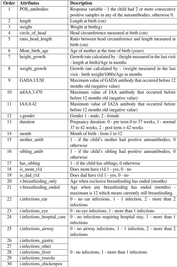
The data set used in this study was built and pre-processed from the original DIPP database and modelled by M.Sc. Oana Maria Stoicescu and most of the variables of the data set used in this is study can be referred to her thesis [64]. The data until the age of 12 months was aggregated to utilise information gain from that data to predict the positivity of the autoantibodies later in life. First, variables such as infections were aggregated to value 0 if the number of infections is zero or to value 1 if more than one or two infections in the first 12 months of age. Infections leading to hospital care and other similar variable were cumulated similarly. Furthermore, for variables such as autoantibodies, the maximum autoantibody value was taken into account before the first positive value before 12 months of age occurred. Later excluded the seven subjects whose autoantibodies values were in positive range before 12 months of age due to autoantibodies transmitted from mother. Finally, a response variable "POS_antibodies" was defined based on the positivity of autoantibodies. Class negative, if the subject never had an occurrence of positive value in any autoantibodies up until 170 months of age and class positive, if the subject had two or more consecutive positive value occurrences in any autoantibodies up until 170 months of age. The value of an autoantibody is positive if they are higher than a specific threshold for the respective autoantibodies. The threshold values for GADA, IA2A, and IAA are 5.34, 0.42, and 3.47, respectively. Overall, providing 30 attributes using a small subset of data of 1329 subjects. Out of which 839 subjects belong to the positive class and
490 to the negative class. Table 3 provides the list of all attributes in the data set and their description. The goal of the data set is to predict the probability of the positivity of autoantibodies before the age of 15 years by utilising information gain from the first 12 months of data.
3.4.2. HAR Using Smartphone Data Set
Recognising and understanding human behaviour using computational artefacts and efforts of applying that information to improve current Human-Centered Computing (HCC) is an emerging research field [65]. Human Activity Recognition (HAR) has also demonstrated to be a significant source of knowledge by accurately identifying human activities for better patient recovery training guidance and could send an early alarm of emergencies such as a stroke or a fall [66]. Combining information gained from a HAR system with other information such as heart rate from a biometric monitoring device can consolidate, for example, the clinical or laboratory investigation and diagnoses and its treatment. The HAR data set used in this study is an open data set, which implies that the data is free and available at the University of California Irvine machine learning repository [16]. The primary intention of the HAR data set collectors was to build models targeting the recognition of six different human activities using smartphones accelerometers and gyroscopes. Moreover, it was made publicly available by being inspired by many other researchers or data collectors of the similar research field.
The motivation of using HAR data set in this study is to utilise a different, big in size, and more complex data set consisting of a rather high correlation between variables. The data set features were derived from raw signals using similar variables which cause the high correlation within the data set. Furthermore, the data set is openly available, so the findings from this study can be replicated or further questioned, which supports the main objective of the study. Therefore, this study examines the performance of the data synthesis tool over the HAR data set towards the possibility of data sharing for similar data sets.
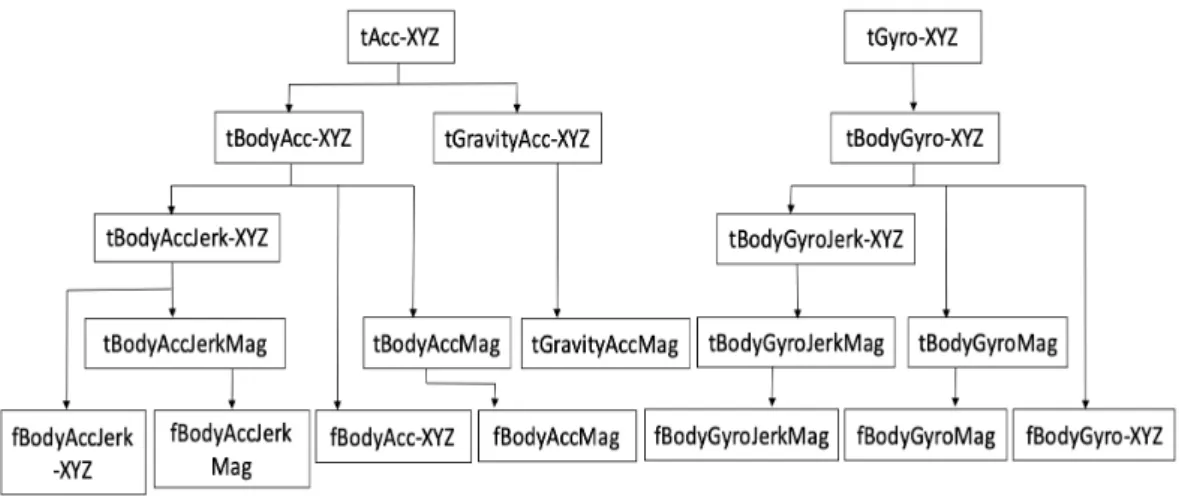
The data set was collected from 30 subjects performing Activities of Daily Living (ADL). The Age group of subjects was 19 to 48 years old, and each subject performed six different activities, including walking, walking upstairs, walking downstairs, sitting, standing, and lying while wearing the Samsung Galaxy S II smartphone on the waist. From the smartphone’s accelerometer and gyroscope, 3-axial raw signals "tAcc-XYZ" and "tGyro-XYZ" at a constant rate of 50Hz were recorded (prefix ’t’ to denote time). Figure 7 represents the workflow of the generation of the signals for feature extraction.
The raw signals collected using the smartphone’s accelerometer and gyroscope sensors were pre-processed for noise reduction using a median filter and a 3rd order low-pass Butterworth filter with a corner frequency of 20 Hz to sample in a fixed-width sliding window of 2.56 seconds with a 50% overlap reaching 128 samples per window. Furthermore, the body acceleration signal "tBodyAcc-XYZ" and gravity acceleration signals "tGravityAcc-"tBodyAcc-XYZ" were acquired using another low-pass Butterworth filter with a cutoff frequency of 0.3 Hz for separating gravitational and body motion component from the acceleration signal. The body linear acceleration (tBodyAcc-XYZ) and angular velocity (tBodyGyro-XYZ)
Figure 7. Signal processing for feature extraction
were derived in the time domain to obtain Jerk signals (tBodyAccJerk-XYZ and tBodyGyroJerk-XYZ). Additionally, the magnitude of these three-dimensional signals was calculated using the Euclidean norm (tBodyAccMag, tGravityAccMag, tBodyAccJerkMag, tBodyGyroMag, tBodyGyroJerkMag). Finally, a Fast Fourier Transform was implemented to some of these signals to generate "fBodyAcc-XYZ", "fBodyAccJerk-XYZ", "fBodyGyro-XYZ", "fBodyAccMag", "fBodyAccJerkMag", "fBodyGyroMag", "fBodyGyroJerkMag". (the prefix ’f’ to indicate frequency domain signals).
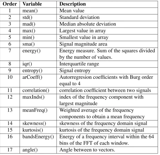
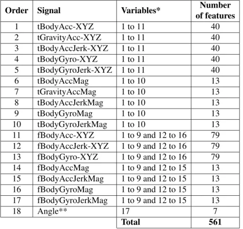
Table 4 list all the variables used for calculating the features from the signals. Table 5 lists all the signals used for feature extraction, including the list of variables used for extraction, ordered according to their occurrence in the data set. To denote the 3-axial signals in the X, Y and Z directions, "-XYZ" is used in the signal naming. From few selected signals, supplementary vectors were obtained by averaging the signals (used later for angle variable from Table 4): gravitymean, tBodyAccMean, tBodyAccJerkMean, tBodyGyroMean, tBodyGyroJerkMean.
Table 6 list last seven features of the data set calculated using the angle between two vectors (Variable 17 in Table 4). Finally, 561 feature vectors were constructed for all six ADL samples for each subject. The complete list of variables of each feature vector is available in’features.txt’file at the University of California Irvine machine learning repository [16].
Table 3. Names and description of attributes
Order Attributes Description
1 POS_antibodies Response variable - 1 the child had 2 or more consecutive positive samples in any of the autoantibodies, otherwise 0. 2 length Length at birth (cm)
3 weight Weight at birth(g)
4 circle_of_head Head circumference measured at birth (cm)
5 ratio_head_length Ratio between head circumference and length measured at birth (cm)
6 Mom_birth_age Age of mother at the time of birth (years)
7 height_growth Growth rate calculated by : (height measured in the last visit - length at birth)/Age in months
8 weight_growth Growth rate calculated by : (weight measured in the last visit - birth weight/1000)/Age in months
9 GADA.UUSI Maximum value of GADA antibody that occurred before 12 months old (negative value)
10 mIAA.3.470 Maximum value of IAA antibody that occurred before before 12 months old (negative value)
11 IAA.0.42 Maximum value of IA2A antibody that occurred before before 12 months old (negative value)
12 s.gender Gender 1 - male, 2 - female
13 duration Pregnancy duration: 0 - pre term 0 to 37 weeks, 1 - normal 37 to 42 weeks, 2 - post term > 42 weeks
14 month Month of birth - from 1 to 12
15 mother_antib 1 - if the child’s mother had positive autoantibodies, 0 otherwise
16 sibling_antib 1 - if the child’s sibling had positive autoantibodies, 0 otherwise
17 has_sibling 1 - if the child has siblings, 0 otherwise 18 is_mom_t1d Does mom have t1d 1 - yes, 0 - no 19 is_dad_t1d Does dad have t1d 1 - yes, 0 - no
20 v.breastfeeding_only Age when exclusive breastfeeding has ended (months) 21 v.breastfeeding_ended Age when any breastfeeding has ended (months)
-maximum is 12 which means currently still breastfeeding. 22 i.infections_ear 0 - no ear infections, 1 - 1 infection, 2 - more than 2
infections
23 i.infections_eye 0 - no eye infections, 1 - more than 1 infections
24 i.infections_hospital_care 0 - no infections requiring hospital stay, 1 - more than 1 infections
25 i.infections_airway 0 - no airway infections, 1 - 1 infection, 2 - more than 2 infections
26 i.infections_gastric
0 - no infections, 1 - more than 1 infections 27 i.infections_other
28 i.infections_fever 29 i.infections_roseola 30 i.infections_chickenpox
Table 4. List of variable used for feature extraction with description Order Variable Description
1 mean() Mean value
2 std() Standard deviation
3 mad() Median absolute deviation 4 max() Largest value in array 5 min() Smallest value in array 6 sma() Signal magnitude area
7 energy() Energy measure. Sum of the squares divided by the number of values.
8 iqr() Interquartile range 9 entropy() Signal entropy
10 arCoeff() Autorregresion coefficients with Burg order equal to 4
11 correlation() correlation coefficient between two signals 12 maxInds() index of the frequency component with
largest magnitude
13 meanFreq() Weighted average of the frequency components to obtain a mean frequency 14 skewness() skewness of the frequency domain signal 15 kurtosis() kurtosis of the frequency domain signal 16 bandsEnergy() Energy of a frequency interval within the 64
bins of the FFT of each window. 17 angle() Angle between to vectors.
Table 5. Summarised list of all the signals used for feature extraction with the variables used. In order corresponding to their occurrence in the data set. *variable represents the order number in Table 4. **detailed list of features using angle in Table 6
Order Signal Variables* of featuresNumber
1 tBodyAcc-XYZ 1 to 11 40 2 tGravityAcc-XYZ 1 to 11 40 3 tBodyAccJerk-XYZ 1 to 11 40 4 tBodyGyro-XYZ 1 to 11 40 5 tBodyGyroJerk-XYZ 1 to 11 40 6 tBodyAccMag 1 to 10 13 7 tGravityAccMag 1 to 10 13 8 tBodyAccJerkMag 1 to 10 13 9 tBodyGyroMag 1 to 10 13 10 tBodyGyroJerkMag 1 to 10 13 11 fBodyAcc-XYZ 1 to 9 and 12 to 16 79 12 fBodyAccJerk-XYZ 1 to 9 and 12 to 16 79 13 fBodyGyro-XYZ 1 to 9 and 12 to 16 79 14 fBodyAccMag 1 to 9 and 12 to 15 13 15 fBodyAccJerkMag 1 to 9 and 12 to 15 13 16 fBodyGyroMag 1 to 9 and 12 to 15 13 17 fBodyGyroJerkMag 1 to 9 and 12 to 15 13 18 Angle** 17 7 Total 561
Table 6. List of last seven features in the data set obtained using angle variable from Table 4 with corresponding vectors. *Index represents the actual index of feature in the data set.
Index* Feature 555 angle(tBodyAccMean,gravity) 556 angle(tBodyAccJerkMean),gravityMean) 557 angle(tBodyGyroMean,gravityMean) 558 angle(tBodyGyroJerkMean,gravityMean) 559 angle(X,gravityMean) 560 angle(Y,gravityMean) 561 angle(Z,gravityMean)
4. EXPERIMENTS AND RESULTS
This chapter reports a comprehensive analysis of the primary tool of data synthesis. The tool has been applied to two different data sets: DIPP and HAR data set. The chapter aims to evaluate whether and to what extent the data synthesis process preserves the general and specific utility along with the quality of the information content of the original data set. First, the performance of the different methods of synthesis is evaluated based on the specific utility of the synthetic data sets to select the fittest method of synthesis. Specific utility compares the performance of the synthetic and original data sets over corresponding data-fitted models and illustrates a visual model comparison based on the FI and their ALE for model fitting. Following the method selection, general utility and the quality of information content is assessed for the selected synthetic data set. The general utility examines the statistical properties of the synthetic data set to the original data set based on the correlation between data variables, data visualisation, data distributions, and data similarity. Whereas, the quality of the information content is measured from an information-theoretic point of view covering entropy and MI within the data sets. Similarly, all three primary analyses are repeated for the HAR data set with the same motivation for general utility and quality of information contained in the data set analyses; however, with additional motivations for specific utility experiments. For HAR data set, the specific utility also measures whether the size of data during data synthesis process affects the performance along with the relevancy of the data synthesis tool for secondary data analysis.
4.1. DIPP Data Set
The pre-processed version of the DIPP data set is a data frame with 30 attributes, including the response variable for 1329 subjects in total. Multiple variables in the data set were first turned into factors using as.factor() command in R. Later, the data set was synthesised numerous times via syn() command from Synthpop package using several methods. As mentioned earlier in Subsection 3.1.2, the first variable to be synthesised in the data is by default generated using "sample" method. In our case, the response variable"POS_antibodies"is the first variable to be synthesised, and then the rest of the attributes. Table 3 provides the list of all attributes in the data set, and their description in the order of synthesis, i.e., "visit.sequence".
Methods of synthesis
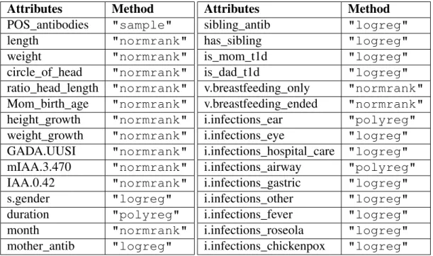
Both non-parametric and parametric methods of synthesis were used in the engendering of the synthetic data sets. Table 7 lists the methods used for generating the corresponding synthetic data with denoting names and method description. Table 8 lists all attributes and corresponding "parametric" method applied. For all non-parametric method, every attribute was synthesised using same method. Each synthetic data set was generated using seed value for result replication. A total of 5 synthetic data sets were generated for initial experimentation using 5 different methods (SynD1 to SynD5). One method of synthesis which performs the best out of
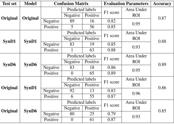
those 5 methods was selected for generating another synthetic data set by setting the argumentpropertoTRUEfor proper synthesis for further analysis (SynD6).
Table 7. Denoted names for synthetic data sets and methods used for creation, *List of parametric method for each variable is listed in Table 8.
Synthetic data Method Description
SynD1 "cart" classification and regression tree
SynD2 "ctree" classification tree
SynD3 "rf" random forest
SynD4 "bag" bagging
SynD5 "parametric" parametric* method to each variable
based on their data type
SynD6 "cart" classification and regression tree
withproperset toTRUE
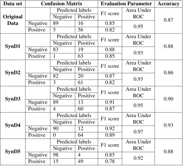
Table 8. Attributes and parametric methods applied for generatingSynD5 data set. Attributes Method POS_antibodies "sample" length "normrank" weight "normrank" circle_of_head "normrank" ratio_head_length "normrank" Mom_birth_age "normrank" height_growth "normrank" weight_growth "normrank" GADA.UUSI "normrank" mIAA.3.470 "normrank" IAA.0.42 "normrank" s.gender "logreg" duration "polyreg" month "normrank" mother_antib "logreg" Attributes Method sibling_antib "logreg" has_sibling "logreg" is_mom_t1d "logreg" is_dad_t1d "logreg" v.breastfeeding_only "normrank" v.breastfeeding_ended "normrank" i.infections_ear "polyreg" i.infections_eye "logreg" i.infections_hospital_care "logreg" i.infections_airway "polyreg" i.infections_gastric "logreg" i.infections_other "logreg" i.infections_fever "logreg" i.infections_roseola "logreg" i.infections_chickenpox "logreg" 4.1.1. Specific Utility
In this section, we evaluated whether different methods of synthesis preserve the specific utility of the original data set differently, after which we selected one method of synthesis that performs best out of all methods used. The goal is twofold, first to investigate if synthetic data sets can be used for machine learning problems when the original data can not be acquired and second to assess how well synthetic data sets perform on the machine learning classifier as compared to the original data set.