ScholarlyCommons
Statistics Papers
Wharton Faculty Research
4-2008
Alpha-Investing: A Procedure for Sequential
Control of Expected False Discoveries
Dean Foster
University of Pennsylvania
Robert A. Stine
University of Pennsylvania
Follow this and additional works at:
http://repository.upenn.edu/statistics_papers
Part of the
Business Commons, and the
Statistics and Probability Commons
This paper is posted at ScholarlyCommons.http://repository.upenn.edu/statistics_papers/13 For more information, please [email protected].
Recommended Citation
Foster, D., & Stine, R. A. (2008). Alpha-Investing: A Procedure for Sequential Control of Expected False Discoveries.Journal of the Royal Statistical Society: Series B: Statistical Methodology, 70(2), 429-444.http://dx.doi.org/10.1111/j.1467-9868.2007.00643.x
Discoveries
Abstract
Alpha-investing is an adaptive, sequential methodology that encompasses a large family of procedures for testing multiple hypotheses. All control mFDR, which is the ratio of the expected number of false rejections to the expected number of rejections. mFDR is a weaker criterion than FDR, which is the expected value of the ratio. We compensate for this weakness by showing that alpha-investing controls mFDR at every rejected hypothesis. Alpha-investing resembles alpha-spending used in sequential trials, but possesses a key difference. When a test rejects a null hypothesis, alpha-investing earns additional probability toward subsequent tests. Alpha-investing hence allows one to incorporate domain knowledge into the testing procedure and improve the power of the tests. In this way, alpha-investing enables the statistician to design a testing procedure for a specific problem while guaranteeing control of mFDR.
Keywords
alpha spending, Bonferroni method, false discovery rate (FDR, mFDR), family-wise error rate (FWER), multiple comparisons
Disciplines
Business | Statistics and Probability
expected false discoveries
Dean P. Foster and Robert A. Stine
∗Department of Statistics
The Wharton School of the University of Pennsylvania
Philadelphia, PA 19104-6340
July 24, 2007
Abstract
Alpha-investing is an adaptive, sequential methodology that encompasses a large family of procedures for testing multiple hypotheses. All control mFDR, which is the ratio of the expected number of false rejections to the expected number of rejections. mFDR is a weaker criterion than FDR, which is the expected value of the ratio. We compensate for this weakness by showing that alpha-investing controls mFDR at every rejected hypothesis. Alpha-investing resembles alpha-spending used in sequential trials, but possesses a key difference. When a test rejects a null hypothesis, alpha-investing earns additional probability toward subsequent tests. Alpha-investing hence allows one to incorporate domain knowledge into the testing procedure and improve the power of the tests. In this way, alpha-investing enables the statistician to design a testing procedure for a specific problem while guaranteeing control of mFDR.
Key words and phrases: alpha spending, Bonferroni method, false discovery rate (FDR, mFDR), family-wise error rate (FWER), multiple comparisons.
∗All correspondence regarding this manuscript should be directed to Prof. Stine at the address shown
with the title. He can be reached via e-mail at [email protected].
1
Introduction
We propose an adaptive, sequential methodology for testing multiple hypotheses. Our approach, called alpha-investing, works in the usual setting in which one has a batch of several hypotheses as well as in cases in which hypotheses arrive sequentially in a stream. Streams of hypotheses arise naturally in contemporary modeling applications such as genomics and variable selection for large models. In contrast to the compara-tively small problems that spawned multiple comparison procedures, modern applica-tions can involve thousands of tests. For example, micro-arrays lead one to compare a control group to a treatment group using measured differences on over 6,000 genes (Dudoit, Shaffer and Boldrick, 2003). If one considers the possibility for interactions, then the number of tests is virtually infinite. In contrast, the example used by Tukey to motivate multiple comparisons compares the means of only 6 groups (Tukey, 1953, available in Braun (1994)). Because alpha-investing tests hypotheses sequentially, the choice of future hypotheses can depend upon the results of previous tests. Thus, hav-ing discovered differences in certain genes, an investigator could, for example, direct attention toward genes that share common transcription factor binding sites (Gupta and Ibrahim, 2005). Genovese, Roeder and Wasserman (2006) describes other testing situations that offer domain knowledge.
Before we describe alpha-investing, we introduce a variation on the marginal false discovery rate (mFDR), an existing criterion for multiple testing. Let the observable random variableR denote the total number of hypotheses rejected by a testing proce-dure, and letV denote the unobserved number of falsely rejected hypotheses. A testing procedure controls mFDR at levelα if
mFDR1 ≡
E(V)
E(R) + 1 ≤α. (1)
mFDR traditionally does not add 1 to the denominator; following our notation, we denote the traditional version mFDR0. The addition of a positive constant to the
denominator avoids statistical problems under the complete null hypothesis. Under the complete null hypothesis, all hypotheses are false, implying, V ≡ R and mFDR0
An investing rule is an adaptive testing procedure that resembles an alpha-spending rule. An alpha-alpha-spending rule begins with an allowance for Type I error, what we call the initial alpha-wealth of the procedure. Each test at level αi reduces the alpha-wealth by αi. Once the alpha-wealth of the spending rule reaches zero, no further tests are allowed. Because the total chance for a Type I error is bounded by the initial alpha-wealth, alpha-spending naturally implements a Bonferroni rule. For multiple testing, however, Bonferroni rules are too conservative. An alpha-investing rule overcomes this conservatism by earning a contribution to its alpha-wealth for each rejected null hypothesis. Thus rejections beget more rejections. Alpha-investing rules further allow one to test an infinite stream of hypotheses, accommodate dependent tests, and incorporate domain knowledge, all the while controlling mFDR.
The sequential nature of alpha-investing allows us to enhance the type of control obtained through mFDR. By placing mFDR in a sequential setting, we can require that a testing procedure does well if stopped early. Suppose rather than testing all m hypotheses, the statistician stops after rejecting 10. We would like to be able to assure her that no more than, say, 2 of these were false rejections, on average. This further protection distinguishes what we call uniform control of mFDR. We show that alpha-investing uniformly controls mFDR.
In general, suppose we test hypotheses until the number of rejections R reaches some target r. Let Tr identify the index of this test. Define V(Tr) to be the number of nulls that have been incorrectly rejected at this point. A test procedure uniformly controls mFDR1 if this stopped process controls mFDR1 in the sense of (1). In words,
equation (1) implies that the expected value ofV given thatR=ris less than or equal toα(r+ 1). This conditional expectation requires that we introduce a stopping time. We defer these details to Section 5. As a preview, we offer
Theorem 1 An alpha-investing rule with control parameters set to α has the property thatE V(Tr)≤α(r+ 1) where Tr is the stopping time defined by occurrence of the rth
rejection andV(m) is the number of false rejections among tests ofm hypotheses.
The rest of this paper develops as follows. We first review several ideas from the literature on multiple comparisons, particularly those related to the family-wise error
rate and false discovery rate (FDR). Next we discuss alpha-investing rules in Section 3. In Sections 4 and 5 we discuss uniform control of mFDR. We describe the design and performance of alpha-investing rules in Section 6. We close in Section 7 with a brief discussion.
2
Criteria and Procedures
Suppose that we havemnull hypothesesH(m) ={H1, H2, . . . , Hm}that specify values for parametersθ={θ1, θ2, . . . , θm}. Each parameterθj can be scalar or vector-valued,
and Θ denotes the space of parameter values. In the most familiar case, each null hypothesis specifies that a scalar parameter is zero,Hj :θj = 0.
We follow the standard notation for labeling correct and incorrect rejections (Ben-jamini and Hochberg, 1995). Assume thatm0 of the null hypotheses inH(m) are true.
TheobservablestatisticR(m) counts how many of thesemhypotheses are rejected. A superscriptθdistinguishesunobservablerandom variables from statistics such asR(m). The random variable Vθ(m) denotes the number of false positives among them tests, counting cases in which the testing procedure incorrectly rejects a true null hypothe-sis. Sθ(m) =R(m)−Vθ(m) counts the number of correctly rejected null hypotheses. Under the complete null hypothesis,m0=m,Vθ(m)≡R(m), andSθ(m)≡0.
The original intent of multiple testing was to control the chance for any false re-jection. The family-wise error rate (FWER) is the probability of falsely rejecting any null hypothesis fromH(m),
FWER(m)≡sup θ∈Θ
Pθ(Vθ(m)≥1). (2) An important special case is control of FWER under the complete null hypothesis: P0(Vθ(m) ≥ 1) ≤ α, where P0 denotes the probability measure under the complete
null hypothesis. We refer to controlling FWER under the complete null hypothesis as controlling FWER in the weak sense.
Bonferroni procedures control FWER. Letp1, . . . , pm denote the p-values of tests of H1, . . . , Hm. Given a chosen level 0< α <1, the simplest Bonferroni procedure rejects
thoseHj for whichpj ≤α/m. Let the indicatorsVjθ∈ {0,1}track incorrect rejections; Vjθ = 1 if Hj is incorrectly rejected and is zero otherwise. Then Vθ(m) =
P Vjθ and the inequality Pθ(Vθ(m)≥1)≤ m X j=1 Pθ(Vjθ = 1)≤α (3) shows that this procedure controls FWER(m)≤α. One need not distributeα equally over H(m); the inequality (3) requires only that the sum of the α-levels not exceed α. This observation suggests an alpha-spending characterization of the Bonferroni procedure. As an alpha-spending rule, the Bonferroni procedure allocates α over a collection of hypotheses, devoting a larger share to hypotheses of greater interest. In effect, the procedure has a budget of α to spend. It can spend αj ≥ 0 on testing each hypothesisHj so long as P
jαj ≤α. Although such alpha-spending rules control FWER, they are often criticized for having little power. Clearly, the power of the traditional Bonferroni procedure decreases as m increases because the threshold α/m for detecting a significant effect decreases. The testing procedure introduced in Holm (1979) offers more power while controlling FWER, but the improvements are small.
To obtain substantially more power, Benjamini and Hochberg (1995) (BH) intro-duces a different criterion, the false discovery rate (FDR). FDR is the expected pro-portion of false positives among rejected hypotheses,
FDR(m) =Eθ Vθ(m) R(m) |R(m)>0 P(R(m)>0). (4) For the complete null hypothesis, FDR(m) = P0(R(m) > 0), which is FWER(m).
Thus, test procedures that control FDR(m) ≤α also control FWER(m) in the weak sense at levelα. If the complete null hypothesis is rejected, FDR introduces a different type of control. Under the alternative, FDR(m) decreases as the number of false null hypothesesm−m0 increases (Dudoit et al., 2003). As a result, FDR(m) becomes more
easy to control in the presence of non-zero effects, allowing more powerful procedures. Variations on FDR include pFDR (which drops the term P(R > 0); see Storey, 2002, 2003) and the local false discovery rate fdr(z) (which estimates the false discovery rate as a function of the size of the test statistic; see Efron, 2005, 2007). Closer to our work, Meinshausen and B¨uhlmann (2004) and Meinshausen and Rice (2006) estimate
m0, the total number of false hull hypotheses in H(m), and Genovese et al. (2006)
weight p-values based on prior knowledge that identifies hypotheses that are likely to be false. Benjamini and Hochberg (1995) also considers mFDR0 and mFDR1, which
they considered artificial. mFDR does not control a property of the realized sequence of tests; instead it controls a ratio of expectations.
Benjamini and Hochberg (1995) also introduces a step-down testing procedure that controls FDR. Order the collection ofm hypotheses so that the p-values of the associ-ated tests are sorted from smallest to largest (putting the most significant first),
p(1) ≤p(2) ≤ · · · ≤p(m) . (5) The test ofH(1)has p-valuep(1), the test ofH(2)has p-valuep(2), and so forth. Ifp(1)> α/m, the BH procedure stops and does not reject any hypothesis. This step controls FWER in the weak sense at levelα. Ifp(1)≤α/m, the procedure rejectsH(1)and moves
on to H(2). Rather than compare p(2) toα/m, however, the BH procedure compares p(2) to 2α/m. In general, the BH step-down procedure rejects H(1), . . . , H(jd−1) for jd= min{j:p(j)> jα/m}. Clearly this sequence of increasing thresholds obtains more
power than a Bonferroni procedure. If the p-values are independent, the inequality of Simes (1986) implies that this step-down procedure satisfies FDR. This sequence of thresholds, however, does not control FWER(m) in general. This is the price we pay for the improvement in power. Subsequent papers (such as Benjamini and Yekutieli, 2001; Sarkar, 1998; Troendle, 1996) consider situations in which the BH procedure controls FDR under certain types of dependence.
3
Alpha-Investing Rules
Alpha-investing resembles alpha-spending used in sequential clinical trials. In a se-quential trial, investigators perform a sequence of tests of one (or perhaps a few) null hypotheses as the data accumulate. An alpha-spending (or error-spending) rule con-trols the level of such tests. Given an overall Type I error rate, say α = 0.05, an alpha-spending rule allocates, or spends, α over a sequence of tests. As Tukey (1991) writes, “Once we have spent this error rate, it is gone.”
While similar in that they allocate Type I error over multiple tests, an alpha-investing rule earns additional probability toward subsequent Type I errors with each rejected hypothesis. Rather than treat each test as an expense that consumes its Type I error rate, an alpha-investing rule treats tests as investments, motivating our choice of name. An alpha-investing rule earns an increment in its alpha-wealth each time that it rejects a null hypothesis. For alpha-investing, Tukey’s remark becomes “Rules that invest the error rate wisely earn more for further tests.” The more hypotheses that are rejected, the more alpha-wealth it earns. If the test of Hj is not significant, however, an alpha-investing rule loses the investedα-level.
More specifically, an alpha-investing ruleIis a function that determines theα-level for testing the next hypothesis in a sequence of tests. We assume an exogenous system external to the investing rule chooses which hypothesis to test next. (Though not part of the investing rule itself, this exogenous system can use the sequence of rejections to pick the next hypothesis.) Let W(k) ≥ 0 denote the alpha-wealth accumulated by an investing rule after k tests; W(0) is the initial alpha-wealth. Conventionally, W(0) = 0.05 or 0.10. At step j, an alpha-investing rule sets the level αj for testing Hj from 0 up to the maximum alpha-level it can afford. The rule must ensure that its wealth never goes negative. LetRj ∈ {0,1} denote the outcome of testingHj:
Rj = 1, ifHj is rejected (pj ≤αj), and 0, otherwise. (6) Using this notation, the investing ruleI is a function ofW(0) and the prior outcomes, αj =IW(0)({R1, R2, . . . , Rj−1}). (7)
The outcome of testingH1, H2, . . . , Hj determines the alpha-wealthW(j) available
for testingHj+1. If pj ≤αj, the test rejects Hj and the investing rule earns a contri-bution to its alpha-wealth, called thepay-out and denoted by ω <1. We typically set α=ω =W(0). Ifpj > αj, its alpha-wealth decreases byαj/(1−αj), which is slightly more than the cost extracted in alpha-spending. The change in the alpha-wealth is thus W(j)−W(j−1) = ω ifpj ≤αj , −αj/(1−αj) ifpj > αj . (8)
If the p-value is uniformly distributed on [0,1], then the expected change in the alpha-wealth is −(1−ω)αj <0. This suggests alpha-wealth decreases when testing a true null hypothesis. Other payment systems are possible; see the discussion in Section 7.
The notion of compensation for rejecting a hypothesis allows one to build context-dependent information into the testing procedure. Suppose that substantive insights suggest that the first few hypotheses are likely to be rejected and that subsequent false hypotheses come in clusters. In this instance, one might consider an alpha-investing rule that invests heavily at the start and after each rejection, as illustrated by the following rule. Assume that the most recently rejected hypothesis isHk∗. (Set k∗ = 0 when testing H1.) If false hypotheses are clustered, an alpha-investing rule should
invest heavily in the test of Hk∗+1. One rule that does this is, forj > k∗,
IW(0)({R1, R2, . . . , Rj−1}) =
W(j−1)
1 +j−k∗ . (9)
This rule invests 1/2 of its current wealth in testing H1 orHk∗+1. Theα-level falls off quadratically if subsequent hypotheses are tested and not rejected. If the substantive insight is correct and the false hypotheses are clustered, then tests of H1 or Hk∗+1 represent “good investments.” An example in Section 6 illustrates these ideas.
While it is relatively straightforward to devise investing rules, it may be difficult
a priori to order the hypotheses in such a way that those most likely to be rejected come first. Such an ordering relies on the specific situation. Another complication is the construction of tests for which one can obtain the needed p-values. To show that a testing procedure controls mFDR, we require that conditionally on the prior j−1 outcomes, the level of the test ofHj must not exceed αj:
∀θ∈Θ, Eθ(Vjθ |Rj−1, Rj−2, . . . , R1)≤αj . (10)
An equivalent statement is that for allθ∈Hj, Pθ(Rj = 1|Rj−1, Rj−2, . . . , R1)≤αj.
The tests need not be independent. Note that the test of Hj is not conditioned on the test statistic (such as a z-score) or parameter estimate. Adaptive testing in a group sequential trial (e.g. Lehmacher and Wassmer, 1999) uses the information on the observed z-statistic at the first look. Tsiatis and Mehta (2003) show that using
this information leads to a less powerful test than procedures that use only acceptance at the first look.
4
mFDR
The following definition generalizes the definition of mFDR given in (1).
Definition 1 Consider a procedure that tests hypotheses H1, H2, . . . , Hm. Then we
define mFDRη(m) = sup θ∈Θ Eθ Vθ(m) Eθ(R(m)) +η . (11)
A multiple testing procedure controls mFDRη(m) at level α if mFDRη(m) ≤ α. We typically set η = 1−α. Values of η near zero produce a less satisfactory criterion. Under the complete null hypothesis, no procedure can reduce mFDR0 below 1 since Vθ(m) ≡ R(m). Control of mFDRη provides control of FWER in the weak sense. Under the complete null hypothesis, mFDRη(m)≤α implies that
Eθ(Vθ(m))≤ α η 1−α .
If η= 1−α, then Eθ(Vθ(m))≤α. Hence, control of mFDR1−α implies weak control of FWER at levelα.
The following simulation illustrates the similarity of mFDRη and FDR. The tested hypothesesHj :µj = 0 specify means ofm= 200 populations. We set µj by sampling a spike-and-slab mixture. The mixture puts 100(1−π1)% of its probability in a spike
at zero; π1 = 0 identifies the complete null hypothesis. The slab of this mixture is a
normal distribution, so that
µj ∼ 0 w.p. 1−π1 N(0, σ2) w.p. π1 . (12)
In the simulation, π1 ranges from 0 (the complete null hypothesis) to 1 (in which
case Vθ(m) ≡ 0). We set σ2 = 2 logm so that the standard deviation of the non-zero µj matches the bound commonly used in hard thresholding. The test statistics
Figure 1: FDR and mFDRη provide similar control. The graph shows the simulated FDR
(solid) and mFDR0.95 (dashed) for the BH step-down procedure (•), oracle-based wBH (?),
Bonferroni (◦), and a procedure that tests each hypothesis at levelα = 0.05(+).
● ● ● ● ● ● ● ● ● ● Proportion False (ππ1) Criterion 0 0.005 0.02 0.08 0.32 1 0 0.01 0.05 0.2 0.5 1 * * * * * * * * * * + + + + + + + + + + ● ● ● ● ● ● ● ● ● ●
are independent, normally distributed random variables Zj iid
∼ N(µj,1) for which the two-sided p-values arepj = 2 Φ(−|Zj|).
Given these p-values, we computed FDR and mFDR0.95 with 10,000 trials of four
test procedures. Two procedures fix the level: one rejects Hj if pj ≤ α = 0.05 and the second rejects ifpj ≤α/200 = 0.00025 (Bonferroni). The other two are step-down tests: the BH and wBH procedures. For our implementation of the wBH procedure, we group the hypotheses into those that are false (µj 6= 0) and those that are true. The hypotheses are weighted so that only false nulls are tested. Each false null receives weight Wj = 1/Sθ(m), and the true nulls get weight zero (see section 3 of Genovese et al., 2006). In effect, it is as though an oracle has revealed which hypotheses are false and the statistician applies the BH procedure to these rather than all m hypotheses.
Figure 1 confirms the similarity of control implied by FDR and mFDR. Both criteria identify the failure of naive testing; FDR and mFDR approach 1 unlessπ1 approaches
1. The criteria also provide similar assessments of the other two procedures; Bonferroni and step-down testing control FDR and mFDR for all levels of signal. Asπ1 increases
and more hypotheses are rejected, both FDR and mFDR of all procedures fall toward zero. The FDR of the wBH procedure is identically zero because it only tests false null hypotheses and cannot incorrectly reject a hypothesis.
5
Uniform control of mFDR
Because alpha-investing proceeds sequentially, the testing can halt after some number of rejected hypotheses. To control such sequential testing, we extend the definition of mF DRη(m) to random stopping times. Recall the definition of a stopping time: T is a stopping time if the eventT ≤j can be determined by information known when the jth test is completed.
Definition 2 If T denotes a finite stopping time of a procedure for testing a stream of hypothesesH1, H2, . . . then mFDRη(T) = sup θ∈Θ Eθ Vθ(T) Eθ(R(T)) +η .
The supremum over stopping times of mFDR determines the uniform mFDR: Definition 3 A testing procedure providesuniform control of mFDRη at level α if
∀(T ∈ T) mFDRη(T)≤α (13)
where T is the set of finite stopping times.
Before proving that alpha-investing provides uniform control of mFDR, we prove half of theorem 1. We first define the relevant stopping time.
Definition 4 The stopping time TR=r ≡ inft{t|R(t) = r} where we take TR=r to be
Lemma 1 For any testing procedure that uniformly controls mFDRα at level α, Eθ Vθ(TR=r)≤α(r+ 1−α).
Proof. Let τ ≥1 denote an arbitrary, but finite, number of tests. We can stop the process at T ≡TR=r∧τ to make it a finite stopping time. Thus Eθ(R(T))≤ r. We know by our hypothesisEθ(Vθ(T))≤α(Eθ(R(T)) + 1−α) =α(r+ 1−α). Since this holds for allτ and Vθ(t) is bounded by r, we can take the limit as r increases.
mFDR and a variety of modifications of FDR become equivalent when stopped at a fixed number of rejections. A bit of algebra shows that
−γR2 ≤mFDR0−FDR−γR ρσV
µR
≤0, (14)
where µV and σV are the mean and standard deviation, respectively, of Vθ(j), the coefficient of variation γR=σR/µR, and ρ is the correlation between Vθ(j) and R(j). When γR is small, FDR and mFDR0 are close. If TR=r is finite almost surely, then the standard deviation of R is identically zero, and hence γR = 0. So, mFDR0 and
FDR are identical. The following theorem is similar in spirit to Tsai, Hsueh and Chen (2003) who work in a Bayesian setting.
Theorem 2 Suppose TR=r < ∞ almost surely. Then a testing procedure that stops
when r rejections have occurred has the following properties: 1. γR= 0.
2. FDR = mFDR0 = cFDR = eFDR = pFDR = E(Vθ(r))/r.
3. FDR ≤αrr+2+1 if the procedure has uniform control of mF DR0 at levelα.
Further, for alpha-investing rules with α=ω=W(0), then 4. Var(Vθ(r))≤α r.
5. P(Vθ(r)≥1 +α r+k√r)≤e−k2/2.
The proofs of all five results are straightforward and hence omitted. Property 5 has a relationship to Genovese and Wasserman (2002, 2004). In Genovese and Wasserman
(2004) a stochastic process of hypothesis tests is considered. Their approach contrasts with ours in that they use a stochastic process indexed by p-values, whereas we use a process indexed by the a priori order in which hypotheses are considered. In both cases, an appropriate martingale converts expectations into tail probabilities.
The following theorem shows that an alpha-investing rule IW(0) with wealth de-termined by (8) controls mFDR1−W(0) so long as the pay-out ω is not too large. The
theorem follows by showing that a stochastic process related to the alpha-wealth se-quenceW(0), W(1), . . .is a sub-martingale. Because the proof of this result relies only on the optional stopping theorem for martingales, we do not require independent tests, though this is the the easiest context in which to show that the p-values are honest in the sense required for (10) to hold.
Theorem 3 An alpha-investing rule IW(0) governed by (8) with initial alpha-wealth
W(0)≤α η and pay-out ω≤α controls mFDRη at levelα.
Theorem 3 also applies to the stopped version of mFDR and hence shows uniform control. A proof of this theorem is in the appendix.
Remark. It may not be obvious that the condition of a finite stopping timeTR=r<
∞ can in fact be met. Given an infinite sequence of hypotheses, define Sθ(∞) = limm→∞Sθ(m). If Sθ(∞) = ∞ then TR=r <∞ for all r because R(m) ≥ Sθ(m). A parameterθ that has the property (for allm and allW(m)>0) that the chance that the alpha-investing procedure I will reject at least one more hypothesis afterm is at least 0.5 is said to providecontinuous funding forI. Clearly for such aθwe have that Sθ(∞) =∞.
We say that an alpha-investing procedure is thrifty if it never commits all of its current alpha-wealth to the current hypothesis. An alpha-investing procedure ishopeful
if it always spends some wealth on the next hypothesis. A hopeful, thrifty procedure consumes some of its alpha-wealth to test every hypothesis in an infinite sequence. With these preliminaries, it can be shown that for any hopeful, thrifty alpha-investing procedure there exists a distributionPθ that provides continuous funding so thatTR=r is finite almost surely.
6
Examples
This section discusses practical issues of using alpha-investing. We start by offering general guidelines, or policies, on how to construct alpha-investing rules. An example constructs an alpha-investing rule that mimics step-down testing. We conclude with simulations that show the advantages of a good policy and compare alpha-investing to BH procedures.
Alpha-investing allows the statistician to incorporate prior beliefs into the design of the testing procedure while avoiding the quagmire of uncorrected multiplicities. This flexibility opens the question of how such choices should be made. We can recommend a few policies.
Best-foot-forward policy. Ideally, the initial hypotheses include those believed most likely to be rejected. For example, in a testing drugs, it is common to test the primary endpoint before others. Alpha-investing rewards this approach: the rejection of the leading hypotheses earns additional alpha-wealth toward tests of secondary endpoints.
Spending-rate policies. Compared to ordering the hypotheses, deciding how much alpha-wealth to spend on each is less important. That said, spending too slowly is inefficient. There is no reward for conserving alpha-wealth unused; the procedure could have used more powerful tests. Alternatively, spending too quickly may exhaust the alpha-wealth before testing every hypothesis. It seems reasonable to use a thrifty procedure that reserves some alpha-wealth for future tests.
Dynamic-ordering policies. Suppose you are lucky enough to have a drug that might cure cancer and heart disease. Clearly, these two hypotheses should be tested first. But what should come next if the procedure rejects one but not the other? The entire collection of subsequent tests depends on which of the initial hypotheses has been rejected. The nature of such dynamic-ordering policies is clearly domain-specific.
Revisiting policies. Our theorems make no assumptions on how the various hy-pothesis are related. This flexibility makes it possible to test hypotheses that
closely resemble others. In fact, our theorems hold if the same hypothesis is tested more than once, so long as subsequent tests condition on prior outcomes. For example, it might be sensible to testHj initially at a small levelαj = 0.001 (so as not to risk much alpha-wealth) and then test other hypotheses. If the test does not rejectHj the first time, it might make sense to test this hypothesis again at a higher level, say, 0.01. In this way, the procedure distributes its alpha-wealth among a variety of hypotheses – spending a little here and then a little there. The following testing procedure illustrates how alpha-investing benefits when the investigator has accurate knowledge of the underlying science. If the investigator can order hypotheses a priori so that the procedure first tests those most likely to be rejected (best-foot-forward policy), then alpha-investing rejects more hypotheses than the step-down test of BH. The full benefit is only realized, however, when combined with a spending-rate policy. Suppose that the test procedure has rejectedHk∗ and is about to test Hk∗+1. Rather than spread its current alpha-wealth W(k∗) evenly over the remaining hypotheses, allocate W(k∗) using a discrete probability mass function such as the following version of (9). This version consumes all remaining alpha-wealth by the last hypothesis by setting
αj = W(j−1) 1 1 +j−k∗ ∨ 1 1 +m−j (15) If a subsequent test rejects a hypothesis, the procedure reallocates its wealth so that all is spent by the time the procedure tests Hm. Mimicking the language of financial investing, we describe this type of alpha-investing rule asaggressive.
In the absence of domain knowledge, a revisiting policy produces an alpha-investing rule that imitates the step-down BH procedure. Begin by investing small amounts of alpha-wealth in the initial test of every hypothesis. This conservative policy means that the procedure runs out of hypotheses well before it runs out of alpha-wealth. To improve its power, the rule uses its remaining alpha-wealth to take a second pass through the hypotheses that were not rejected in the first pass. Although we do not advocate this as a general procedure, it is allowed by our theorems. Gradually “nibbling” away at the hypotheses in this fashion results in a procedure that resembles
step-down testing. In fact, as the size of these nibbles goes to zero, the order that hypotheses are rejected is precisely that from step-down testing. The point where each testing procedure stops is slightly different. Sometimes step-down testing stops first and sometimes alpha-spending stops first.
A few calculations clarify the connection to the BH procedure. To avoid taking many passes through the hypotheses without generating any rejects, increase the size of the nibbles so as to take as large a bite each time as possible. Set α =ω =W(0). The procedure begins by testing each hypothesis in H(m) at level β1 =α/(α+m)≈ α/m, approximating the Bonferroni level. This level assures us that the procedure exhausts its alpha-wealth if no hypothesis is rejected. If, however, some hypothesis is rejected, the procedure uses the earned alpha-wealth to revisit the hypotheses that were not rejected in the first pass. At the start of each pass, the algorithm divides its alpha-wealth equally among all remaining unrejected hypotheses and tests each at this common level. These steps continue until a pass does not reject a hypothesis and the alpha-wealth reaches zero.
On successive passes through the hypotheses, the fact that a hypothesis was previ-ously tested must be used in computing the rejection region. Suppose that exactly one hypothesis is rejected at each pass. In the first pass, the p-value of one hypothesis is smaller than the initial levelβ1. Following (8), the rule paysβ1/(1−β1) for each test
that it does not reject and earns α for rejecting H(1). Hence, after the initial test of each hypothesis at level β1, the alpha-wealth grows slightly to
W(m) = W(0) +ω−(m−1)β1/(1−β1)
= α+α/m (16)
For largem, its alpha-wealth is virtually unchanged fromW(0).
For the second pass, the procedure again distributes its alpha-wealth equally over the remaining hypotheses. The level invested in each test at this second pass is
β2 =
W(m)
W(m) +m−1 > α m .
To determine which tests are rejected during the second pass, assume that the remain-ing p-values are uniformly distributed. Conditionremain-ing onpj > β1, this pass rejects any
hypothesis for whichpj ≤p∗ with the thresholdp∗ determined by P0(pj ≤p∗ |pj > β1) =
p∗−β1
1−β1
=β2 .
This implies that p∗ =β1+β2−β1β2 ≈2α/m. Thus, the second pass approximately
rejects any hypotheses with p-value is smaller than 2α/m, the second threshold of the step-down test. In this way, the investing rule gradually raises the threshold for rejecting hypotheses as in step-down testing. If any hypothesis is rejected during a pass over the remaining hypotheses, then alpha-wealth remains and the testing procedure continues recursively. Instead of spending equally on each hypothesis one could weight these hypotheses differently. This idea of using prior information is implicit in alpha-spending rules. The use of prior information also appears in the wBH procedure proposed in Genovese et al. (2006). Following the ideas of this section, we can show that the wBH procedure controls mFDR.
Simulations. Our first simulation compares three alpha-investing rules to step-down versions of the BH and wBH procedures. As in Section 3 for the wBH procedure, an oracle assigns weights
Wj = 0 ifHj is true 1/Sθ(m) otherwise,
to each hypothesis so that wBH only tests false hypotheses. For the sake of comparison, each replication of the simulation tests a fixed batch of m = 200 hypotheses. The 200 hypotheses are defined as in the simulation in Section 3 (see equation 12); this simulation also uses 10,000 samples. Of the alpha-investing rules, one implements the revisiting policy that mimics the BH procedure. The other two alpha-investing rules implement aggressive alpha-investing. To illustrate the impact of domain knowledge, we simulated the performance of alpha-investing using (15) in a best-case and a worst-case scenario. For the best worst-case, the investigator tests the hypotheses in the order implied by|µj|, testing the hypothesis with the largest|µj|first. The tests are ordered by the underlying means rather than the observed p-values. In the worst case, the hypotheses are tested in random order, indicating poor domain knowledge. We set the
Figure 2: Comparison of the FDR and power of aggressive alpha-investing rules with accurate
(O) and inaccurate (M) domain knowledge to BH (•), oracle-based wBH (?), and a revisiting
alpha-investing rule (◦). (a) All five procedures control FDR. (b) Better domain knowledge
improves the power of alpha-investing relative to step-down testing. The vertical axis shows the ratio of the number of correctly rejected null hypotheses relative to BH.
● ● ● ● ● ● ● ● ● ● Proportion False (ππ1) FDR 0 0.005 0.02 0.08 0.32 1 0 0.01 0.02 0.03 0.04 0.05 * * * * * * * * * * ● ● ● ● ● ● ● ● ● ● * * * * * * * * * Proportion False (ππ1) Power Relative to BH 0.005 0.02 0.08 0.32 1 0.5 1 1.5 2 ● ● ● ● ● ● ● ● ● ● ● ● ● ● ● ● ● ●
level for all procedures toα= 0.05; for alpha-investing, the initial wealthW(0) =α=ω and η= 1−α.
Figure 2(a) shows the FDR of each procedure. As in the prior simulation summa-rized in Figure 1, FDR and mFDR are quite similar in this simulation and so we have only shown FDR. All five procedures control FDR (and mFDR), as they should. As in Figure 1, the FDR of the wBH procedure is identically zero because it tests only false null hypotheses. For the other procedures that do not benefit from this oracle, it becomes easier to control FDR in the presence of more false null hypotheses (larger π1). Accurate domain knowledge reduces the FDR of the aggressive procedure. When
tested in random order (poor domain knowledge), the FDR of aggressive testing is similar to that of the BH step-down procedure.
does it find signal? For each alpha-investing rule, Figure 2(b) shows the ratio of the number of correctly rejected hypotheses relative to the number rejected by BH, estimating Eθ Sθ(200,test procedure) Sθ(200,BH)
from the simulation. With accurate domain knowledge, aggressive alpha-investing rejects in excess of 50% more hypotheses than the step-down BH procedure. Unless the problem offers few false null hypotheses (π1 < 0.02, an average of 1 or 2 false
null hypotheses), aggressive alpha-investing with good domain knowledge obtains the greatest power. Alpha-investing gains more from testing the hypotheses in the right order than BH gains from knowing which hypotheses to test. If the domain knowledge is poor, aggressive alpha-investing rejects no less than 70% of the number rejected by step-down testing. As expected from its design, alpha-investing using the revisiting policy performs similarly to step-down testing.
We also performed a simulation to investigate the performance of alpha-investing when applied to an infinite stream of hypotheses. Each null hypothesis specifies a mean (Ht:µt= 0, t= 1,2, . . .), and the test statistic for each hypothesis is Zt∼N(µt,1), independently. The simulation computes the FDR and power of aggressive alpha-investing using the rule (9) and a two-sided test ofHt. Two levels of signal are present in the simulation. Under one scenario, 10% of the null hypotheses are false; in the second, 20% are false. For each scenario, false null hypotheses cluster in bursts of varying size. We generated the sequence of means µt from a two-state Markov chain
{Yt}. In state 0, the null hypothesis holds, µt = 0. In state 1,µt= 3. The transition probabilities for the Markov chain are pij = P(Yt+1 = j | Yt = i). The probability
of leaving state 0 varies over p01 = (0.0025,0.005,0.010,0.025,0.05). To obtain a
fixed percentage of false null hypotheses, we set p10 = k p01 with k = 4 (20% false
null hypotheses) and k = 9 (10%). Given k, increases in the transition probability p01 produce a more choppy sequence of hypotheses. We simulated 1,000 streams of
hypotheses for each combination of k and p01, beginning each with Y1 = 1 (a false
null). As in previous simulations, we set W(0) =α=ω = 0.05 andη = 1−α.
aggressive alpha-investing is thrifty and hopeful in the sense of Section 5, it can be shown that the sequence of means{µt}generated by the Markov chain do not provide continuous funding. Each sequence of tests eventually stops after a finite number of tests when the alpha-wealth runs out. Even so, at the point of the snapshot in Figure 3, each simulated realization of alpha-investing has enough alpha-wealth to reject further hypotheses. For example, the retained alpha-wealth W(4000) averaged 0.003 with k = 9 and p01 = 0.05 (fewest, most choppy false hypotheses) up to 0.63 with k = 4
and p01= 0.0025. In every case, Figure 3(a) shows that the FDR lies well below 0.05.
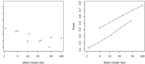
Figure 3(b) shows that aggressive alpha-investing has higher power when applied to sequences with a higher proportion of false null hypotheses that arrive in longer clusters. This situation affords the best opportunity to accumulate alpha-wealth that can be spent quickly to reject clustered false hypotheses. The power rises rapidly once a cluster of false null hypotheses is discovered. For example, the overall power is 0.51 withk= 4 andp01= 0.025 (20% false nulls with mean cluster size 10). For finding the
first null hypothesis of each cluster, however, the power falls to 0.20. This observation suggests that a revisiting policy that returns to hypotheses immediately preceding a rejected hypothesis would have higher power. In general, the power shown in Figure 3(b) rises roughly linearly in the log of the mean cluster size 1/p10. Aggressive
alpha-investing also finds a higher percentage of the false null hypotheses when more are present. The power is consistently higher when 20% of the hypotheses are false (k = 4) than when 10% are false (k = 9). The gap between these scenarios diminishes slightly as the mean cluster size increases. As in the prior simulation, the higher power obtained for longer clusters is accompanied by smaller rates of false discoveries.
7
Discussion
The best-foot-forward policy raises a concern relevant to any multiple testing procedure that controls an FDR-like criterion. Suppose thatH(m) is contaminated with trivially-false hypotheses that artificially produce alpha-wealth. Then all subsequent tests are tainted. As an extreme example, suppose the first hypothesis claims “gravity does not
Figure 3: The power of aggressive alpha-investing increases with a higher proportion of false null hypotheses that arrive in longer clusters. The frames show (a) FDR after completing
4,000 tests and (b) power (◦denotes 10% false nulls (k= 9) and×, 20% false nulls (k = 4)).
● ● ● ● ● 2 5 10 20 50 100 0.038 0.042 0.046 0.050
Mean Cluster Size
FDR ● ● ● ● ● 2 5 10 20 50 100 0.1 0.2 0.3 0.4 0.5 0.6 0.7 0.8
Mean Cluster Size
Power
exist.” After rejecting this hypothesis, the testing procedure has more alpha-wealth to use in subsequent tests than allocated by W(0). Most readers would, however, be uncomfortable using this additional alpha-wealth to test the primary endpoint of a drug. Step-down tests share this problem. By rejecting the trivially falseH1, the level
of the test of the first “real hypothesis” is 2α/mrather than α/m. In this sense, it is important to allow an observer to ignore the list of tested hypotheses from some point onward. The design of the sequential test procedure should put the most interesting hypotheses first to insure that that when the reader stops, they have seen the most important results. By providing uniform control of mFDR, alpha-investing controls this criterion wherever the observer stops.
One can regulate alpha-investing using other methods of compensating, or charging, for each test. The increment in the alpha-wealth defined in (8) is natural, with a fixed reward and penalty determined by whether the test rejects a hypothesis, say Hj. Because neither the payout ω nor the cost α/(1−α) reveals pj (other than to
indicate ifpj ≤αj), subsequent tests need only condition on the sequence of rejections, R1, . . . , Rj. The following alternative method for regulating alpha-investing has the same expected pay-out, but varies the winnings when the test rejectsHj:
W(j)−W(j−1) = ω+ log(1−pj) ifpj ≤αj , log(1−αj) ifpj > αj . (17)
Alpha-investing governed by this “regulator” also satisfies the theorems shown previ-ously. Because the reward revealspj when Hj is rejected, however, the investing rule must condition onpj for any rejected prior hypotheses. This would seem to complicate the design of tests in applications in which the p-values are not independent. Other methods for regulating the alpha-wealth could be desirable in other situations. We hope to pursue these ideas in future work.
We speculate that the greatest reward from developing a specialized testing strategy will come from developing methods that select the next hypothesis rather than specific functions to determine howα is spent. The rule (15) invests half of the current wealth in testing hypotheses following a rejection. One can devise other choices. Results in information theory (Rissanen, 1983; Foster, Stine and Wyner, 2002), however, suggest that one can find universal alpha-investing rules. A universal alpha-investing rule would reject on average as many hypotheses as the best rule within some class. We would expect such a rule to spend its alpha-wealth more slowly than the simple rule (15), but retain this general form.
Appendix
Proof of Theorem 3
We begin by defining a stochastic process indexed byj, the number of hypotheses that have been tested:
Our main lemma shows that A(j) is a sub-martingale for alpha-investing rules with pay-outω ≤α. In other words we will show thatA(j) is “increasing” in the sense that
Eθ(A(j)|A(j−1), A(j−2), . . . , A(1))≥A(j−1).
Theorem 3 uses the weaker fact thatEθA(j)≥A(0). By definitionVθ(0) =R(0) = 0 so thatA(0) =η α−W(0)≥0 ifW(0)≤η α. WhenA(j) is a sub-martingale, the optional stopping theorem implies that for all finite stopping timesM thatEθA(M)≥0. Thus,
Eθ
α(R(M) +η)−Vθ(M) = Eθ(W(M) +A(M))
≥ EθA(M)
≥ A(0)≥0.
The first inequality follows because the alpha-wealth W(j)≥0 [a.s.], and the second inequality follows from the sub-martingale property. Thus, once we have shown that A(j) is a sub-martingale, it follows that EθVθ(M)≤α(EθR(M) +η) and
mFDRη(M) =
EθVθ(M) EθR(M) +η
≤α. Thus to show Theorem 3 we need to prove the following lemma:
Lemma 2 Let Vθ(m) andR(m)denote the cumulative number of false rejections and the cumulative number of all rejections, respectively, when testing a sequence of null hypotheses {H1, H2, . . .} using an alpha-investing rule IW(0) with pay-out ω ≤α and
alpha-wealth W(m). Then the process
A(j) ≡ αR(j)−Vθ(j) +η α−W(j)
is a sub-martingale,
Eθ(A(m)|A(m−1), . . . , A(1))≥A(m−1). (18) Proof. Write the cumulative counts Vθ(m) andR(m) as sums of indicatorsVjθ, Rj ∈ {0,1}, Vθ(m) = m X j=1 Vjθ, R(m) = m X j=1 Rj .
Similarly write the accumulated alpha-wealthW(m) andA(m) as sums of increments, W(m) =Pm
j=0Wj and A(m) =
Pm
j=0Aj. Let αj denote the alpha level of the test of Hj that satisfies the condition (10). The change in the alpha-wealth from testing Hj can be written as:
Wj =Rjω−(1−Rj)αj/(1−αj), Substituting this expression forWj into the definition of Aj we get
Aj = (α−ω)Rj−Vjθ+ (1−Rj)αj/(1−αj).
Since Rj ≥0 and α−ω ≥0 by the conditions of the lemma, it follows that
Aj ≥(1−Rj)αj/(1−αj)−Vjθ . (19)
Ifθj 6∈Hj, thenVjθ = 0 andAj ≥0 almost surely. So we only need to consider the case in which the null hypothesisHj is true. WhenHj is true, Rj ≡Vjθ and (19) becomes
Aj ≥(1−Rj)αj/(1−αj)−Rj = (αj−Rj)/(1−αj). (20) Abbreviate the conditional expectation
Eθj−1(X) =Eθ(X |A(1), A(2), . . . , A(j−1)) .
Under the null, Eθj−1Rj ≤αj by the definition of this being an αj level test. Taking conditional expectations in (20) gives Eθj−1Aj ≥0.
References
Benjamini, Y. and Hochberg, Y. (1995) Controlling the false discovery rate: a practical and powerful approach to multiple testing. Journal of the Royal Statist. Soc., Ser. B,57, 289–300.
Benjamini, Y. and Yekutieli, D. (2001) The control of the false discovery rate in multiple testing under dependency. Annals of Statistics,29, 1165–1188.
Braun, H. I. (ed.) (1994) The Collected Works of John W. Tukey: Multiple Compar-isons, vol. VIII. New York: Chapman & Hall.
Dudoit, S., Shaffer, J. P. and Boldrick, J. C. (2003) Multiple hypothesis testing in microarray experiments. Statistical Science,18, 71–103.
Efron, B. (2005) Selection and estimation for large-scale simultaneous infer-ence. Tech. rep., Department of Statistics, Stanford University, http://www-stat.stanford.edu/brad/papers/.
— (2007) Size, power, and false discovery rates. Annals of Statistics,35, to appear. Foster, D. P., Stine, R. A. and Wyner, A. J. (2002) Universal codes for finite sequences
of integers drawn from a monotone distribution. IEEE Trans. on Info. Theory,48, 1713–1720.
Genovese, C., Roeder, K. and Wasserman, L. (2006) False discovery control with p-value weighting. Biometrika,93, 509–524.
Genovese, C. and Wasserman, L. (2002) Operating charateristics and extensions of the false discovery rate procedure. Journal of the Royal Statist. Soc., Ser. B, 64, 499–517.
— (2004) A stochastic process approach to false discovery control.Annals of Statistics, 32, 1035–1061.
Gupta, M. and Ibrahim, J. G. (2005) Towards a complete picture of gene regulation: using Bayesian approaches to integrate genomic sequence and expression data. Tech. rep., University of North Carolina, Chapel Hill, NC.
Holm, S. (1979) A simple sequentially rejective multiple test procedure. Scandinavian Journal of Statistics,6, 65–70.
Lehmacher, W. and Wassmer, G. (1999) Adaptive sample size calculations in group sequential trials. Biometrics,55, 1286–90.
Meinshausen, N. and B¨uhlmann, P. (2004) Lower bounds for the number of false null hypotheses for multiple testing of associations under general dependence.
Biometrika,92, 893–907.
Meinshausen, N. and Rice, J. (2006) Estimating the proportion of false null hypotheses among a large number of independently tested hypotheses. Annals of Statistics,34, 373–393.
Rissanen, J. (1983) A universal prior for integers and estimation by minimum descrip-tion length. Annals of Statistics,11, 416–431.
Sarkar, S. K. (1998) Some probability inequalities for ordered Mtp2 random variables:
A proof of the Simes conjecture. Annals of Statistics,26, 494–504.
Simes, R. J. (1986) An improved bonferroni procedure for multiple tests of significance.
Biometrika,73, 751–754.
Storey, J. D. (2002) A direct approach to false discovery rates. Journal of the Royal Statist. Soc., Ser. B,64, 479–498.
— (2003) The positive false discovery rate: a Bayesian interpretation and the q-value.
Annals of Statistics,31, 2013–2035.
Troendle, J. F. (1996) A permutation step-up method of testing multiple outcomes.
Biometrics,52, 846–859.
Tsai, C.-A., Hsueh, H.-m. and Chen, J. J. (2003) Estimation of false discovery rates in multiple testing: Application to gene microarray data. Biometrics,59, 1071 – 1081. Tsiatis, A. A. and Mehta, C. (2003) On the inefficiency of the adaptive design for
monitoring clinical trials. Biometrika,90, 367–378.
Tukey, J. W. (1953) The problem of multiple comparisons. Unpublished lecture notes. — (1991) The philosophy of multiple comparisons. Statistical Science,6, 100–116.