Theses & Dissertations Boston University Theses & Dissertations
2019
Pathway activity analysis of bulk
and single-cell RNA-Seq data
https://hdl.handle.net/2144/34809
AND
COLLEGE OF ENGINEERING
Dissertation
PATHWAY ACTIVITY ANALYSIS OF BULK AND SINGLE-CELL RNA-SEQ DATA
by
DAVID FOWLER JENKINS III
Sc.B., Brown University, 2011 M.S., Boston University, 2017
Submitted in partial fulfillment of the requirements for the degree of
Doctor of Philosophy 2019
© 2019
David Fowler Jenkins III All rights reserved
First Reader _________________________________________________________ W. Evan Johnson, Ph.D.
Associate Professor of Medicine and Biostatistics
Second Reader _________________________________________________________ Joshua D. Campbell, Ph.D.
iv
DEDICATION
To my grandparents
v
ACKNOWLEDGMENTS
My thesis work would not have been possible without a team of people helping me along the way, so I’d like to say thank you. First and foremost, to my advisor Evan, whose infectious enthusiasm I felt from the first day we met in 2014. I left every meeting with you inspired to work hard, and I won’t ever forget that, thank you. To my
collaborators, particularly Andrea Bild, Moom Rahman, and Shelley MacNeil, I’m proud of the work we did together, thank you. To my fellow lab mates, especially Tyler,
Supriya, Mani, Yuqing, and Jason, thanks for your positive feedback and support. To my thesis committee, Paola, Josh, Jen, and Masanao, thanks for your suggestions and
flexibility, it was a pleasure to work with you. To the BU Bioinformatics program, particularly Caroline Lyman, Johanna Vasquez, and David King, you have been more than generous with your time and resources; we all really appreciate the work you do to make our graduate work go as smoothly as possible. To my friends, both old and new, for always being there to make me laugh or listen to me when I needed you, thank you. Finally, to my family, Dave, Caroline, Emma, Sam, Gram L, and Paula, I love you.
vi
PATHWAY ACTIVITY ANALYSIS OF BULK AND SINGLE-CELL RNA-SEQ DATA
DAVID FOWLER JENKINS III
Boston University Graduate School of Arts and Sciences and College of Engineering, 2019
Major Professor: W. Evan Johnson, Associate Professor of Medicine and Biostatistics ABSTRACT
Gene expression profiling can produce effective biomarkers that can provide additional information beyond other approaches for characterizing disease. While these approaches are typically performed on standard bulk RNA sequencing data, new methods for RNA sequencing of individual cells have allowed these approaches to be applied at the resolution of a single cell. As these methods enter the mainstream, there is an increased need for user-friendly software that allows researchers without experience in bioinformatics to apply these techniques. In this thesis, I have developed new, user-friendly data resources and software tools to allow researchers to use gene expression signatures in their own datasets. Specifically, I created the Single Cell Toolkit, a user-friendly and interactive toolkit for analyzing single-cell RNA sequencing data and used this toolkit to analyze the pathway activity levels in breast cancer cells before and after cancer therapy. Next, I created and validated a set of activated oncogenic growth factor receptor signatures in breast cancer, which revealed additional heterogeneity within public breast cancer cell line and patient sample RNA sequencing datasets. Finally, I created an R package for rapidly profiling TB samples using a set of 30 existing
vii
of tuberculosis treatment failure samples. Taken together, the results of these studies serve as a set of user-friendly software tools and data sets that allow researchers to rapidly and consistently apply pathway activity methods across RNA sequencing samples.
viii
TABLE OF CONTENTS
DEDICATION ... iv
ACKNOWLEDGMENTS ... v
ABSTRACT ... vi
TABLE OF CONTENTS ... viii
LIST OF TABLES ... xiv
LIST OF FIGURES ... xv
LIST OF ABBREVIATIONS ... xviii
Chapter 1. Introduction ... 1
Transcriptional Regulation and Disease ... 1
Transcriptional Pathways in Cancer ... 2
Tuberculosis ... 2
RNA Sequencing ... 3
Single-Cell RNA Sequencing ... 4
Dissertation Aims ... 4
Aim 1: Create a user-friendly interface and a full-featured analysis toolkit for single-cell RNA-Seq datasets ... 5
Aim 2: Create and apply oncogenic growth factor receptor network signatures across breast cancer cell lines and breast cancer patient tumor samples ... 5
ix
Aim 3: Collect available biomarkers of tuberculosis disease and progression, create an analysis framework to apply these signatures, and profile the pathway activity in
a cohort of tuberculosis treatment failure samples ... 6
Chapter 2. An analysis toolkit for single-cell RNA-Seq data ... 7
Introduction ... 7
Methods ... 9
Mucosal-associated Invariant T (MAIT) Cells ... 9
Pluripotent Stem Cells ... 9
Data Structure ... 10
Data Upload ... 11
Data Summary and Filtering ... 12
Dimensionality Reduction and Clustering ... 14
ComBat Batch Correction ... 15
Differential Expression and Biomarker Creation ... 15
Subsampling and Differential Power Analysis ... 17
Pathway Activity Analysis ... 17
Results ... 18
Data Upload ... 19
Data Summary and Filtering ... 21
Dimensionality Reduction ... 24
Differential Expression with MAST ... 26
Pathway Activity Analysis with GSVA ... 29
x
Discussion ... 35
Software Availability ... 36
Acknowledgments ... 36
Chapter 3. Oncogenic growth factor receptor network signatures in TCGA and metastatic breast cancer ... 37
Introduction ... 37
Methods ... 45
Overexpression of genes of interest in human mammary epithelial cells ... 45
Western blot analysis for expression of growth factor proteins in HMECs and apoptotic proteins in breast cancer cell lines ... 46
Dose response assay ... 47
RNA preparation and RNA sequencing ... 49
Gene expression data processing, normalization, and datasets ... 49
Generation of gene expression signatures ... 50
Gene set enrichment analysis on RNA-Seq signatures ... 51
Batch adjustment and estimation of pathway activity in ICBP and TCGA BRCA patient samples ... 52
Optimization of single-pathway estimates in ICBP cell line and TCGA BRCA patient data ... 53
Software implementation of pathway activity prediction with generated signatures 57 Determination of growth factor phenotypes in ICBP and TCGA ... 57
Identification of additional drug response heterogeneity within growth factor phenotypes ... 57
xi
Statistical analyses ... 58
Results ... 59
Two dominant phenotypes in breast cancer patients and cell lines ... 59
GFRN phenotypes and subgroups contribute to variation found in TCGA breast cancer gene expression data ... 66
Breast cancer growth phenotypes bifurcate in expression of mitochondrial apoptotic proteins ... 70
GFRNs predict drug response in breast cancer ... 74
Discussion ... 80
Conclusion ... 84
Acknowledgments ... 84
Funding ... 84
Availability of Data and Materials ... 85
Author Contributions ... 85
Competing Interests ... 85
Ethics Approval and Consent to Participate ... 85
Chapter 4. Pathway signature profiling of tuberculosis RNA-Seq data ... 86
Introduction ... 86
Methods ... 87
Sample Processing and Sequencing ... 87
RNA-Seq Data Analysis ... 88
Collection of Published TB Signatures ... 89
xii
Gene Set Analysis ... 91
Visualization ... 92
Software Availability ... 93
Results ... 94
Previously published TB signatures show decreased TB signature activity at month two in TB failure samples ... 94
Existing signatures of TB fail to distinguish TB treatment failures at baseline ... 97
No significantly differentially expressed genes separated baseline controls and TB treatment failures ... 101
Discussion ... 103
Acknowledgments ... 105
Chapter 5. Conclusion ... 106
APPENDIX A: Cell lines used in the independent drug assay and the Western blotting experiments. ... 108
APPENDIX B: Gene list of optimized gene numbers determined for each GFRN signature. ... 110
20 Gene AKT Signature ... 110
250 Gene BAD Signature ... 110
50 Gene EGFR Signature ... 111
10 Gene HER2 Signature ... 111
100 Gene IGF1R Signature ... 112
xiii
200 Gene RAF Signature ... 113
LIST OF JOURNAL ABBREVIATIONS ... 116
BIBLIOGRAPHY ... 120
xiv
LIST OF TABLES
Table 2.1. Comparison of SCTK and other popular scRNA-Seq analysis tools. ... 8
Table 2.2. Table of summary metrics produced by the summarizeTable() function. .. 23
Table 3.1. Drug dose information for the drug response assay. ... 48
Table 3.2. -log(EC50) drug sensitivity values from the dose response assay. ... 49
Table 3.3. ASSIGN parameters used for all analyses. ... 53
Table 3.4. Spearman correlations for protein correlations. ... 56
Table 4.1. AUC Values and 95% confidence intervals for pathway activity predictions using GSVA scores to predict failure samples. ... 98
xv
LIST OF FIGURES
Figure 2.1. Single Cell Toolkit upload tab. ... 20
Figure 2.2. Single Cell Toolkit Data Summary and Filtering tab. ... 22
Figure 2.3. Single Cell Toolkit Dimensionality Reduction and Clustering tab. ... 25
Figure 2.4. Result of plotTSNE() on the MAIT dataset. ... 26
Figure 2.5. Single Cell Toolkit MAST tab. ... 27
Figure 2.6. MAST result visualizations available in the SCTK. ... 29
Figure 2.7. Single Cell Toolkit Pathway Activity Analysis tab. ... 30
Figure 2.8. Pathway activity heatmap from the gsvaPlot() function. ... 31
Figure 2.9. PCA before and after ComBat batch correction. ... 32
Figure 3.1. High-level overview for probing growth factor receptor networks in breast cancer. ... 42
Figure 3.2. Validation of protein overexpression for each GFRN signature. ... 45
Figure 3.3. Gene expression signatures for key GFRN pathways generated by ASSIGN. ... 50
Figure 3.4. GFRN gene expression signature validations in TCGA breast cancer data. ... 54
Figure 3.5. Analysis of pathway activity and intrinsic subtypes. ... 61
Figure 3.6. Pathway activity estimates between ER+ and ER- samples in breast cancer cell lines and patient data. ... 62
Figure 3.7. Pathway activation estimates across clinical subtypes. ... 63
Figure 3.8. Pathway activation estimates across intrinsic subtypes. ... 64
Figure 3.9. Survival analysis of the four subgroups in TCGA BRCA samples (N=1,119). ... 66
xvi
Figure 3.10. Correlation between mean gene expression values for all samples and PC 1 values ... 68 Figure 3.11. Principal component analysis across TCGA breast tumors. ... 69 Figure 3.12. Survival and growth phenotypes differ in cell survival mechanisms. ... 72 Figure 3.13. Independent western blot assay for MCL-1 and BIM proteins between breast cancer cell lines from the survival and growth phenotypes. ... 73 Figure 3.14. Growth factor receptor network phenotypes reflect dichotomous drug
response in breast cancer cell lines. ... 75 Figure 3.15. Differential drug response identified in GFRN phenotype heterogeneity. ... 77 Figure 3.16. Correlations between pathway activation estimates and drug response values between ER+ and ER- and between HER+ and HER2- samples in breast cancer cell lines. ... 79 Figure 3.17. Summary of the survival and growth phenotypes in breast cancer. ... 80 Figure 4.1. Overlap of genes in the TB signature cohort listed in 5 or more signatures. .. 89 Figure 4.2. Scaled GSVA pathway activity scores for baseline failure, baseline control,
and month two failure samples. ... 94 Figure 4.3. Pathway activity scores from month two failure samples. ... 95 Figure 4.4. Boxplot of ACS_COR signature scores in combined India failure and Leong
et al. India datasets. ... 96 Figure 4.5. ROC Curves of ACS_COR and FAILURE signatures in baseline samples. .. 98 Figure 4.6. Heatmap of row scaled log(TPM) gene expression data for the FAILURE
xvii
Figure 4.7. GSEA enrichment of 13-gene failure signature on baseline samples using gene set enrichment analysis. ... 100 Figure 4.8. GSVA pathway activity scores for FAILURE signature in baseline Thompson
et al. samples. ... 101 Figure 4.9. Differentially expressed genes at baseline as identified by DESeq2. ... 102
xviii
LIST OF ABBREVIATIONS
ANOVA ... Analysis of variance AR ... Androgen receptor ASSIGN ... Adaptive Signature Selection and InteGratioN ATCC ... American Type Culture Collection AUC ... Area under the curve BAD ... Bcl-2-associated death promoter BC ... Breast cancer BCA ... Bicinchoninic acid BCL-2 ... B-cell lymphoma 2 gene BRCA ... Breast cancer cDNA ... Complementary DNA CDR ... Cellular detection rate CLARA ... Clustering for Large Applications CPM ... Counts per million DE ... Differential expression DMSO ... Dimethyl sulfoxide DNA ... Deoxyribonucleic acid DOTS ... Directly observed treatment short course strategy EC50 ... Concentration of a drug that gives half-maximal response EGFR ... Epidermal growth factor receptor EBI ... European Bioinformatics Institute EDTA ... Ethylenediaminetetraacetic acid
xix
EMT ... Epithelial–mesenchymal transition ER ... Estrogen receptor FBS ... Fetal bovine serum FDR ... False discovery rate FISH ... Fluorescence in situ hybridization FPKM ... Fragments per kilobase million GEO ... Gene Expression Omnibus GFP ... Green fluorescent protein GFRN ... Growth factor receptor network GSEA ... Gene Set Enrichment Analysis GSVA ... Gene Set Variation Analysis GUI ... Graphical user interface HER2 ... Human epidermal growth factor receptor 2 HMECs ... Human primary mammary epithelial cells ICBP ... Integrative Cancer Biology Program IGF1R ... Insulin-like growth factor 1 receptor IHC ... Immunohistochemistry KEGG ... Kyoto Encyclopedia of Genes and Genomes LOOCV ... Leave-one-out cross-validation LTBI ... Latent tuberculosis infection MAIT ... Mucosal associated invariant T cell MAPK ... Mitogen-activated protein kinase MAST ... Model-based analysis of single-cell transcriptomics
xx
MCL-1 ... Induced myeloid leukemia cell differentiation protein Mcl-1 gene MEBM ... Mammary epithelial basal medium mRNA ... Messenger RNA MSigDB ... The Molecular Signatures Database mTOR ... Mammalian target of rapamycin NA ... Not available NCBI ... National Center for Biotechnology Information PAM50 ... Point accepted mutation 50 matrix PBS ... Phosphate-buffered saline PC ... Principal component PCA ... Principal component analysis PI3K ... Phosphoinositide 3-kinase PR ... Progesterone receptor PVDF ... Polyvinylidene difluoride RNA ... Ribonucleic acid RNA-Seq ... RNA sequencing ROC ... Receiver operating characteristic RPPA ... Reverse phase protein array RTK ... Receptor tyrosine kinase scRNA-Seq ... Single-cell RNA sequencing ssGSEA ... Single sample gene set enrichment analysis SCTK ... Single Cell Toolkit SDS ... Sodium dodecyl sulfate
xxi
t-SNE ... T-distributed stochastic neighbor embedding TB ... Tuberculosis TCGA ... The Cancer Genome Atlas TNBC ... Triple negative breast cancer TPM ... Transcripts per kilobase million UCSC ... University of California, Santa Cruz
Chapter 1. Introduction
Transcriptional Regulation and Disease
It is well established that cell signaling plays an important role in disease (Nahta, Hortobágyi & Esteva, 2003). The cell is a highly regulated and carefully controlled machine, with many signaling pathways working together to address the needs of each cell (Schlessinger, 2000). When these pathways are disrupted, there can be devastating effects. When attempting to quantify these changes in pathway activity there are several levels to probe. Alterations in DNA (DNA mutations) can cause changes in pathway activity, deactivating or activating a specific transcription factor, but redundancy in transcription factor pathways means that not every mutational event will have a strong, if any, effect (Spitz, Furlong, 2012). Further, many DNA mutations occur in positions in the genome that have no effect, so sifting through many mutations to identify the causal change is often difficult. An alternative approach is to quantify RNA expression. Messenger RNA (mRNA) is the transcriptional language that converts the instructions coded in DNA into protein products. By quantifying the level of RNA expression for each gene in a specific sample, a picture of the cellular activity of these genes can be identified. Differences in the levels of gene expression across samples can point to the causes of disease phenotypes or be used as a biomarker of a specific disease state. Often these biomarkers are not a single value, but a set of coordinately expressed genes that form a signature that can represent the activity of a cellular component, such as a pathway. By identifying biomarkers of disease, we can stratify patients into groups with similar cellular activity, which can often respond to disease treatments in similar ways (Groenendijk, Bernards, 2014, McCubrey et al., 2012).
Transcriptional Pathways in Cancer
In cancer, activating or inactivating mutations can disrupt the cell signaling cascades that control how cells grow, divide, and undergo apoptosis (McCubrey et al., 2012). These changes in cell signaling networks have become an important part of the set of ‘hallmarks of cancer,’ causing cells to grow uncontrollably, form tumors, and
metastasize (Hanahan, Weinberg, 2011). Cancer is one of the leading causes of death globally with an estimated 18.1 million new cases in 2018 (The International Agency for Research on Cancer, 2018). Fortunately, targeted cancer drugs to address specific
abnormalities in cancer signaling pathways have been developed (Gustafson et al., 2010). These targeted drugs can inhibit certain signaling pathways driven by key oncogenic growth factor receptors, such as EGFR and HER2 (Nahta, Hortobágyi & Esteva, 2003). Importantly, by identifying the signaling cascade that is driving a specific tumor, drugs that target components of that pathway can be administered. The ultimate goal of pathway analysis in cancer is to identify a set of biomarkers that can precisely
characterize the drivers of a specific tumor and identify the drugs that would best target the exact combination of aberrations in a specific patient’s tumor, an approach commonly known as personalized medicine.
Tuberculosis
Tuberculosis (TB) infection is a leading cause of death worldwide (World Health Organization, 2016). The majority of patients infected with TB will not progress to active TB disease (World Health Organization, 2016). Of those that do get infected, some will fail their treatment. In TB, many gene signatures have been produced that can accurately predict the likelihood of TB progression or predict active TB disease (Zak et al., 2016,
Sambarey et al., 2017, Leong et al., 2018). These pathways typically contain genes involved in the immune and inflammatory responses (Scriba et al., 2017). Similar to their use in cancer, gene signatures of TB can help stratify patients into groups that are likely to progress to disease and those that are unlikely to get disease, monitor patient adherence to drug regimens, and ensure that infections are being successfully treated. This could be particularly important in situations where TB drugs are scarce, or resources for TB treatment are reduced, and help improve outcomes for TB treatment.
RNA Sequencing
RNA sequencing leverages high throughput sequencing technologies to quantify the gene expression levels in a sample. Standard sequencing pipelines involve aligning reads to a reference genome and counting the number of genes that overlap with each gene or transcript annotation. These raw counts can then be normalized to correct for differences in sequencing depth between samples or corrected for unwanted experimental variations called batch effects (Johnson, Li & Rabinovic, 2007) . The normalized counts can then be merged into a matrix of counts per sample for downstream analysis, which often involves identifying significantly differentially expressed pathways or gene
signatures. Within the R programming language, several software tools have been created to make the storage of gene expression data easier. The SummarizedExperiment object allows for storage of multiple matrices which can be used to store sample and gene annotation data along with raw and normalized count data (Huber et al., 2015) . The object can be subset, automatically subsetting the annotation data along with the count data to make sure everything remains in sync.
Single-Cell RNA Sequencing
Typical bulk RNA sequencing combines the expression of genes from all cells in a sample. Recently, new techniques for performing single-cell RNA-Seq have been developed. These techniques involve either physically separating cells into individual wells in a plate or performing highly multiplexed bead-based library preparation for higher throughput results (Picelli et al., 2013, Macosko et al., 2015). The end result is expression data for an individual cell, allowing researchers to probe differences in gene expression across cell types or tumor subgroups. Due to the low amount of starting material for each individual cell, scRNA-Seq shows lower gene expression levels than typical bulk RNA-Seq datasets and some genes display a bimodal pattern of expression. To address these concerns, additional filtering and normalization steps are needed before standard RNA-Seq analysis techniques can be performed on scRNA-Seq datasets
(Brennecke et al., 2013). Further, novel analysis methodologies that take into account the missingness that typically arises in scRNA-Seq data have been developed (Finak et al., 2015, Trapnell et al., 2014, Satija et al., 2015). Choosing which analysis methods to use can be dataset specific, and often involves iterating through several analysis techniques before settling on the best approach for a given dataset.
Dissertation Aims
The aims in this dissertation seek to develop novel software frameworks and pathway signatures to aid in the analysis of bulk and single-cell RNA-Seq datasets in the context of disease, specifically breast cancer and tuberculosis. Together, these aims will show that by creating interactive and intuitive tools for data processing, users can perform sophisticated analysis on RNA-Seq datasets without needing to write code or
have a deep understanding of how to run the standard underlying algorithms for RNA-Seq analysis.
Aim 1: Create a user-friendly interface and a full-featured analysis toolkit for single-cell RNA-Seq datasets
Many tools for performing single-cell RNA-Seq (scRNA-Seq) analysis exist, but these tools are often only available on the command line and require significant
bioinformatics expertise to use. While other software tools for analysis and visualization exist, there has yet to be a full scRNA-Seq analysis tool to help users take raw data through a standard pipeline to produce downstream analysis including quality control and filtering, visualization with dimensionality reduction methods, differential expression analysis, and pathway activity and gene enrichment approaches. In this aim, I present the Single Cell Toolkit (SCTK), the first fully interactive scRNA-Seq analysis tool written in R and Shiny. This tool allows users to perform a full scRNA-Seq analysis pipeline through an intuitive point-and-click interface, allowing improved access to scRNA-Seq analysis tools.
Aim 2: Create and apply oncogenic growth factor receptor network signatures across breast cancer cell lines and breast cancer patient tumor samples
Cell line derived gene expression signatures have been used to identify signatures of pathway activity in cancer samples (Bild et al., 2006). These signatures can then be used to stratify samples by cellular activity and predict the effectiveness of drugs that target activated oncogenic pathways. In this aim, I describe a new set of pathway activity signatures of breast cancer oncogenes in growth factor receptor networks. Pathway
activity predictions were performed using Adaptive Signature Selection and Integration (ASSIGN) and can be run automatically through extensions of the ASSIGN R package (Shen et al., 2015). This set of signatures was applied to cancer cell line panels and patient breast cancer tumor samples, revealing additional heterogeneity within the cohorts and significant correlations to differences in drug response.
Aim 3: Collect available biomarkers of tuberculosis disease and progression, create an analysis framework to apply these signatures, and profile the pathway activity in a cohort
of tuberculosis treatment failure samples
Several signatures of TB have been previously published and can accurately predict several aspects of TB progression into active disease or predict the effectiveness of TB treatment. Since numerous unique signatures have been developed, it is worthwhile to explore differences in pathway activity across several signatures rather than looking at them individually. In this aim, a set of 30 previously published gene signatures of TB were collected. To rapidly profile this set of 30 gene signatures we created the TB Signature Profiler, a software framework to easily profile a set of samples with a set of user defined signatures using common pathway activity prediction algorithms. With this tool, users can profile and visualize the pathway activity predictions easily, leveraging the SummarizedExperiment object within R to store raw data and pathway activity scores together. We used the TB Signature Profiler on a set of TB samples from treatment failure patients and identified heterogeneity that showed the published signatures can accurately show TB treatment response and highlight issues with adherence to drug treatment.
Chapter 2. An analysis toolkit for single-cell RNA-Seq data
Adapted from the following manuscript:
David F. Jenkins, Tyler Faits, Mohammed Muzamil Khan, Emma Briars, Sebastian Carrasco Pro, Steve Cunningham, Joshua D. Campbell, Masanao Yajima, and W. Evan Johnson. (Manuscript submitted)
Introduction
Single-cell RNA sequencing (scRNA-Seq) techniques allow researchers to explore the transcriptional landscape of a sample at the resolution of the individual cell. In the context of cancer, scRNA-Seq can identify the subclonality of a tumor sample to improve our ability to identify the cell-specific mechanisms that drive tumor growth and can characterize different cellular populations within the tumor microenvironment (Tirosh et al., 2016, Brady et al., 2017). However, different optimizations of parameters and algorithms are required for filtration, normalization, clustering, and differential expression of scRNA-Seq data compared to bulk RNA-Seq due to the low amount of starting material and technical bias introduced in the common scRNA-Seq library preparation techniques (Brennecke et al., 2013). Tools for normalization and analysis of scRNA-Seq data exist to overcome these technical biases, but these tools are not
integrated and require command line processing of samples and knowledge of the many options available for each tool, which makes them difficult to use, especially for
scientists without training in bioinformatics (McCarthy et al., 2017, Nakamura et al., 2015, Satija et al., 2015, Kharchenko, Silberstein & Scadden, 2014, Fan et al., 2016, Trapnell et al., 2014). Even for more advanced users, there is still a need to interactively
explore scRNA-Seq results during processing to help make dataset specific decisions that can affect downstream analysis.
Shiny is an R package and toolkit developed by RStudio
(https://www.rstudio.com) that allows for the creation of web based graphical user
interfaces (GUIs) over R packages, allowing for interactive data exploration and analysis through familiar drop down menus and buttons (Chang et al., 2017). Users can load a Shiny app locally on their computer or the Shiny app can be hosted in the cloud and can be accessed through a web browser.
Package SCATER SC3 SEURAT SCDE PAGODA MONOCLE SCTK
Filtering and Data
Summary ü ü ü Dimensionality Reduction ü ü ü ü Clustering ü ü ü ü ü Batch Correction ü ü ü ü Differential Expression ü ü ü ü ü Pathway Enrichment ü ü ü Experimental Design ü GUI ü ü ü ü SingleCellExperiment Support ü ü ü
Table 2.1. Comparison of SCTK and other popular scRNA-Seq analysis tools. While SCATER (McCarthy et al., 2017), SC3 (Nakamura et al., 2015), SEURAT (Satija et al., 2015), SCDE (Kharchenko, Silberstein & Scadden, 2014) , PAGODA (Fan et al., 2016), and MONOCLE (Trapnell et al., 2014) accomplish some steps in the scRNA-Seq analysis pipeline, the SCTK supports a full interactive scRNA-Seq analysis workflow and supports the SingleCellExperiment object for data storage.
Here, we present the Single Cell Toolkit (SCTK), an R/Shiny based package for both command line and interactive scRNA-Seq processing. While other tools can perform specific scRNA-Seq analysis steps, the SCTK is the first fully interactive scRNA-Seq analysis workflow available within the R language (Table 2.1). We applied the SCTK and our workflow on multiple data examples, including stimulated and unstimulated mucosal-associated invariant T cells, induced pluripotent stem cells from Yoruba male
reference samples to identify batch effects, and tumor cells from breast cancer patients to identify pathway activity in response to treatment (Tung et al., 2017, Finak et al., 2015, Brady et al., 2017).
Methods
The SCTK is organized into several analysis modules. All modules can be run interactively through the Shiny web interface or through the R console. Below we
describe the datasets available in the SCTK, the underlying architecture of the SCTK, and the analysis modules available through the interactive SCTK package and GUI.
Mucosal-associated Invariant T (MAIT) Cells
To demonstrate how interactive analysis can be performed in the SCTK, an example dataset of mucosal-associated invariant T (MAIT) cells was used
(Finak et al., 2015). A set of 96 CD8+ MAIT cells were sorted, 47 cells were stimulated with cytokines, and the cells were processed and sequenced using the Fluidigm C1 system. The data was aligned to the human genome, quantified, and included with the MAST package. Cytokine stimulation of MAIT cells results in increased cytokine gene expression and pathway activity changes that can be identified with differential
expression analysis and pathway activity analysis, which can serve as an effective control for our toolkit methods if cytokine genes and cytokine containing pathways are identified through analysis.
Pluripotent Stem Cells
A dataset demonstrating batch effects in single-cell data was created by Tung, et. al (Tung et al., 2017). Three induced pluripotent stem cell lines were sequenced in
triplicate on the Fluidigm C1 platform using a total of 9 plates. The resulting data has a clear plate effect that represents an experimental batch effect that could affect
downstream analysis if it is not corrected. After removing the batch effect, the
experimental replicates should not separate during analysis, allowing the data to be used to identify biological differences between the individuals.
Data Structure
Steps in the analysis pipeline are performed on a SCTKExperiment object, an extension of the SingleCellExperiment and RangedSummarizedExperiment objects developed by the Bioconductor project (Huber et al., 2015). This object is organized into identically sized matrices designed to store counts, normalized counts, or batch corrected data; a data frame for sample annotation information; and a data frame for feature
annotation information. These objects allow users to keep their scRNA-Seq data organized in a single object that automatically resizes all matrices and annotation information if the data is modified, ensuring annotation information and count data is always in sync. Additionally, data from dimensionality reduction approaches such as principal component analysis (PCA) and t-distributed stochastic neighbor embedding (t-SNE) can be stored in the object’s reducedDims slot. The SingleCellExperiment object has been optimized to store large datasets by using sparse matrices and an efficient API to support data that would otherwise not fit into memory using a standard matrix (Lun, Pagès & Smith, 2018). Depending on the size of the data stored in the object, the matrices used in the object are automatically stored as either standard R matrices, sparse matrices, or on disk as a HDF5 file backed matrix. This allows users to take advantage of these memory saving strategies automatically without needing to specify which type of matrix
that should be used on their dataset. The SingleCellExperiment can also store information about spike-in transcripts and sample specific size factors for normalization. By utilizing an object that can efficiently store both raw data and downstream analysis results, analysis can be performed within the SCTK, saved into the object, and loaded into R for additional analysis on the command line.
The SCTKExperiment is implemented as an S4 object, an object-oriented system available within R. This allows users to inherit methods and structure that exists in other S4 objects and add additional functionality while still being backwards compatible. The SCTKExperiment object also stores the percent variation explained by each principal component. This is accomplished by adding an additional slot named pcaVariances to the SCTKExperiment object that stores the percent variation explained by each principal component (PC) as a DataFrame. The getPCA() function available in the SCTK saves
the PCs into the reducedDims slot and additionally stores the percent variation explained in the pcaVariances slot. This data can be accessed using the pcaVariances() function.
The SCTKExperiment object can be further extended and will continue to be expanded in future versions of the SCTK to store additional single-cell data, annotations, and results.
Data Upload
After installing the SCTK, users can start the Shiny app by running the
singleCellToolkit() function with a SCTKExperiment object as an input to
automatically load the data into the app. Alternatively, a user can choose to upload a data matrix of raw count or normalized data directly through the Shiny app by uploading a text file, along with optional sample and feature annotation files. The SCTK will create a
SCTKExperiment object to store the toolkit analysis results. This object can be exported after analysis has been completed.
Data Summary and Filtering
After scRNA-Seq data has been loaded into the SCTK, a table of data summary metrics is presented. Because scRNA-Seq data is very sparse, dataset specific filtration and normalization can affect downstream analysis (Stegle, Teichmann & Marioni, 2015). In the data summary and filtering tab, the SCTK provides users with several summary statistics and options for manipulating their data and annotation information. First, within the Data Summary subtab, the SCTK displays a table of summary metrics including the number of samples, number or genes, average number of reads per cell, average number of genes per cell, and the number of genes with few or no counts across all samples. Additionally, histograms of the number of counts per sample and the number of
expressed genes per sample are displayed. If the dataset is small, containing less than 50 cells, the entire data matrix is also displayed. Using this information, the user can make decisions about how best to filter their data for downstream analysis. Users can filter genes and samples with low or no expression, delete outlier samples, filter the dataset based on annotation information, and modify the annotation information by uploading a replacement annotation matrix. For larger datasets, users can also randomly subset their data on this tab, allowing the user to perform exploratory analysis on a reduced dataset within the SCTK. The filtering applied while using this tab modifies the underlying data that is used throughout the app. A snapshot of the original uploaded data is preserved so a user can always return to the original uploaded data to restart the analysis or try a
The SCTK doesn’t require users to import their data with a specific set of gene annotation information, but some tools within the SCTK are only available if the data uses specific gene annotations. Depending on the reference genome that is used during sequence alignment and quantification, users may have data that describes their genes using gene symbols (e.g. BRCA1), Entrez gene numeric IDs from the NCBI database (e.g. 672 for BRCA1), Ensembl gene IDs from the EBI (e.g. ENSG00000012048 for BRCA1), or from another source. The SCTK has the ability to convert gene ids to various formats using the org.*.eg.db Bioconductor annotation packages. These packages are not installed by default, so these must be manually installed before this function will work. After these packages have been installed, users can convert between the available gene annotations on the Data Summary and Filtering tab.
Additional modifications to the underlying data object are available in the Assay Details subtab. Lists of the available data matrices and reduced dimension data are displayed in the Assay Details tab. Users can add additional data matrices to their data object. Any existing matrix can be log-transformed, or if raw count data is available, a counts per million (CPM) normalization can be applied. Unwanted data matrices or reduced dimensionality can be deleted in this tab.
Finally, in the Visualize subtab, users can visualize gene expression data versus annotation data for genes of interest using a boxplot, scatterplot, barplot, or heatmap depending on the type of annotation data information that is available. This can be helpful for visualizing housekeeping genes for sample quality control, quantifying artificial spike-in controls for sequencing quality control, or visualizing individual genes of interest.
Dimensionality Reduction and Clustering
Visualization of scRNA-Seq data is crucial to identifying subclusters of cells present in the data. Dimensionality reduction techniques allow a user to visualize scRNA-Seq data by summarizing the observed variation into lower dimension space. PCA transforms the matrix into components that describe the variation observed in the data. An alternative to PCA, t-distributed stochastic neighbor embedding (t-SNE), is also frequently used when analyzing scRNA-Seq data because it is able to embed a large amount of variation into a small number of dimensions (Van, Hinton, 2008). When users open the dimensionality reduction and clustering tab in the SCTK, a list of available reduced dimension datasets and algorithms is provided. Because these algorithms can take a long time to compute on large datasets, users can precompute the reduced
dimension data and store it in a SCTKExperiment object before uploading the data into the SCTK. For smaller datasets, users can perform PCA and t-SNE directly through the SCTK app. The resulting reduced matrices will be stored in the underlying object that can be downloaded when analysis is complete. The resulting data can be displayed in the dimensionality reduction and clustering tab. Annotation information can be added to the plot by selecting annotations with which to color or shape the points in the scatterplot.
After visualization of the data, users may want to stratify the scRNA-Seq data into clusters that appear during dimensionality reduction. Users can choose to cluster their data using k-means clustering, hierarchical clustering, or CLARA (Clustering for Large Applications). Clustering is typically performed on the PCA data, because t-SNE data does not retain the distance between clusters in its results. After the clustering algorithm is complete, the plot is automatically updated to display the resulting clusters. If the user
wants to save the cluster results, the cluster assignments can be stored in the annotation data frame of the SCTKExperiment object and visualized on other reduced dimension data. Additionally, other clustering algorithms can be run on the command line, saved as annotation information in the SCTKExperiment object, and visualized in this tab.
ComBat Batch Correction
Because of the complexities of the library preparation and the low starting material in scRNA-Seq experiments, non-biological variation (batch effects) are present and can be a major source of variation present in single-cell experiments (Hicks et al., 2017). ComBat is a widely used method for adjusting for batch effects in microarray and RNA-Seq data (Johnson, Li & Rabinovic, 2007). If users identify variation associated with a technical effect, ComBat can be run within the SCTK to remove this variation before further downstream analysis. Users can choose an annotation present in the annotation data frame and add additional covariates to the ComBat model before
performing batch correction. After batch correction, the ComBat results are stored as an additional assay in the SCTKExperiment object, which can then be used in the other analysis tabs within the SCTK.
Differential Expression and Biomarker Creation
Differential expression analysis can identify genes that are significantly up or down regulated between conditions. While many differential expression algorithms exist, their performance may vary on scRNA-Seq datasets. Users can apply common
differential expression algorithms limma (Ritchie et al., 2015), DESeq2 (Love, Huber & Anders, 2014), or perform an ANOVA to identify differentially expressed genes by
selecting one or multiple condition variables present in the annotation information. Users can customize the differential expression results by changing the number of genes to return, the p-value significance cutoff, and the p-value correction method applied to the results. The resulting gene list is displayed as a table and also in a heatmap which can also be customized. Users can download the gene list directly or create a biomarker list for a specific cell type or cell cluster, which can be stored in the gene annotation information in the SCTKExperiment object.
Single-cell RNA-Seq specific tools for differential expression have been developed that can adjust for some of the characteristics of scRNA-Seq data. MAST, Model-based Analysis of Single-cell Transcriptomics, has been developed to address these issues by using a hurdle model (Finak et al., 2015). A hurdle model allows for separate accounting of the processes that produce zero count values, and the ones that produce the positive count values. MAST allows users to identify this cutoff by using an adaptive threshold model that bins genes based on gene expression and identifies a cutoff for zero expression. This allows the dropout rate typical of scRNA-Seq data to be
modelled. Additionally, MAST models the cellular detection rate (CDR), a measure of the percent of genes that are expressed in a given sample. Adding the CDR to the model can correct for biological and technical covariates when identifying differences in the condition of interest. MAST has been implemented within the SCTK. Users can choose whether to use MAST’s adaptive thresholding model, choose fold change and expression thresholds, and identify significant genes based on conditions present in the annotation information provided. The results are presented in a table, violin plots, or visualized in a
heatmap and can be saved as a biomarker in the SCTKExperiment object or downloaded directly.
Subsampling and Differential Power Analysis
The relative complexity of scRNA-Seq experimental designs makes it difficult for investigators to ensure that an experiment will have sufficient power while operating on a finite budget. Whereas there are tools for optimizing bulk RNA-Seq designs (Busby et al., 2013, Guo et al., 2014), these fail to account for the tiered nature of scRNA-Seq experiments, where each biological replicate may contribute any number of cells to be sequenced, each of which may belong to one of many cell types or subpopulations. Users of the SCTK can project estimated power metrics based on their dataset with variable simulated parameters including sequencing depth, number of sequenced cells, and number of biological replicates. To produce results within a reasonable timespan, the Shiny interface only allows users to vary one parameter at a time while keeping the others fixed. The command line allows users to probe all parameters at once, producing multidimensional power estimates which will help investigators optimize their scRNA-Seq experimental designs.
Pathway Activity Analysis
Gene expression measurements can be summarized into a signature or set of genes to create a score that represents the activity of that set of genes in a sample. By summarizing genes in known signaling pathways, cells with active signaling pathways or specific cellular functions can be identified. Gene Set Variation Analysis (GSVA) uses gene sets to create these signatures (Hänzelmann, Castelo & Guinney, 2013). The
molecular signature database (MSigDb) is a database of molecular signatures that can be used in GSVA (Liberzon et al., 2011). GSVA has been implemented in the SCTK. Users can select their input data, gene set(s), and GSVA parameters interactively through the app. GSVA can be run across all MSigDB signatures, a user selected subset of MSigDB signatures, or a set of custom gene signatures saved as annotation columns in the
rowData slot of the SCTKExperiment object. After GSVA is complete, scores will be displayed in either violin plots or a heatmap on the Pathway Activity tab of the SCTK. Users can save the pathway activity scores into the annotation data columns of the SCTKExperiment object or download the scores directly.
Results
The SCTK allows users to analyze data interactively through the Shiny web interface, or perform command line analysis and visualize the results when the analysis is complete. Interactive analysis works best for smaller studies of several hundred cells, which typically come from plate-based technologies such as SMART-Seq or CEL-Seq where cells are physically sorted into 96-well plates (Picelli et al., 2013, Hashimshony et al., 2016). For larger datasets, such as those created through commercially available tools such as the 10x Chromium Single Cell Solution and other droplet-based high throughput methods, analysis modules in the SCTK can be run on the command line, saved in the SCTKExperiment object, and loaded into the toolkit for efficient visualization (Macosko et al., 2015). To demonstrate a standard analysis workflow in the SCTK, two example datasets will be used. Equivalent analysis will be shown through the interactive modules and through the functions available on the R console.
Data Upload
To demonstrate how interactive analysis can be performed in the SCTK, we will begin using the MAIT cell example. The MAIT cell example should separate by
experimental condition (cytokine stimulated vs unstimulated) and genes identified
through differential expression and pathways identified through pathway activity analysis should be associated with cytokine stimulation.
To upload data into the toolkit for interactive analysis, data was extracted from the MAST package and the TPM matrix, sample annotations, and gene annotations were saved as tab separated text files. After starting the SCTK, the data can be uploaded on the “Upload” tab by selecting the text files and clicking upload (Figure 2.1). Optionally, the user can select “Create log(counts) assay” to store both the originally uploaded counts and a log transformed matrix.
Figure 2.1. Single Cell Toolkit upload tab. Users can choose between uploading data through file upload boxes or preloaded example datasets. When the user clicks the ‘Upload’ button, the app creates a SCTKExperiment object to store raw data and analysis.
To perform analysis using the R functions available in the SCTK, the MAST data first must be loaded into a SCTKExperiment object. This can be accomplished with the
createSCE() function.
R> library(MAST)
R> library(singleCellTK) R> library(xtable)
R> data(maits, package="MAST")
R> maits_sce <- createSCE(assayFile = t(maits$expressionmat), + annotFile = maits$cdat,
+ featureFile = maits$fdat, + assayName = "logtpm", + inputDataFrames = TRUE, + createLogCounts = FALSE)
Data Summary and Filtering
On the second tab in the interactive toolkit, a table of summary metrics is rendered. Additionally, the user is provided with several options for filtering data and modifying the underlying SCTKExperiment object. The MAIT dataset contains an annotation column called “ourfilter.” The “Filter samples by annotation” filter was used to subset the original dataset of 96 cells to remove all cells that do not pass the filter, leaving 74 cells (Figure 2.2). This filter subsets all data assays, cell annotation data, and gene annotation data present in the SCTKExperiment object. The singleCellTK has the ability to convert gene ids to various formats in the “Convert Gene Annotation” section of the data summary and filtering page by selecting the organism, the source annotation type, and the annotation type to convert the gene annotations to.
Figure 2.2. Single Cell Toolkit Data Summary and Filtering tab. In the right panel, a table of data summary metrics and a heatmap of counts per sample is displayed. The original 96 cells in the MAIT data are filtered to remove all samples that do not pass the “ourfilter” annotation column in the dataset using the “Filter samples by annotation” filter. 74 pass filter cells remain. Additional tools for data filtering are available in the left column.
In the R console, the summarizeTable() function produces summary metrics
from a SCTKExperiment object. The user selects the assay to summarize and the table of summary metrics is produced (Table 2.2). Typically, these summary statistics would be run on a "counts" matrix, but the MAIT SCTKExperiment object only contains log(tpm) values so the average number of reads per cell is calculated from the normalized values instead of raw counts.
R> summarizeTable(maits_sce, useAssay = "logtpm")
Number of Samples 96 Number of Genes 16302 Average number of reads per cell 17867 Average number of genes per cell 6833 Samples with <1700 detected genes 5 Genes with no expression across all samples 0
Table 2.2. Table of summary metrics produced by the summarizeTable() function. Five of the 96 cells in the MAIT dataset have fewer than 1,700 detected genes, indicating that these cells may have failed sequencing and should be removed for downstream analysis.
Sample annotation information is available in the colData data frame in the SCTKExperiment object. The “ourfilter” annotation can be used to subset the data within the SCTKExperiment object.
R> summarizeTable(maits_sce, useAssay = "logtpm") R> colnames(colData(maits_sce))
[1] "wellKey" "condition" "nGeneOn"
[4] "libSize" "PercentToHuman" "MedianCVCoverage" [7] "PCRDuplicate" "exonRate" "pastFastqc"
[10] "ncells" "ngeneson" "cngeneson" [13] "TRAV1" "TRBV6" "TRBV4" [16] "TRBV20" "alpha" "beta" [19] "ac" "bc" "ourfilter" R> table(colData(maits_sce)$ourfilter) FALSE TRUE 22 74
To convert gene annotations in the R console, the convertGeneIDs() function
can be used. Annotations can be converted between various formats available within the org.*.eg.db Bioconductor annotation packages which must be installed separately.
R> library(org.Hs.eg.db)
R> maits_entrez <- maits_subset
R> maits_subset <- convertGeneIDs(maits_subset, inSymbol = "ENTREZID", + outSymbol = "SYMBOL",
+ database = "org.Hs.eg.db")
Dimensionality Reduction
Next, the data is visualized in the Dimensionality Reduction and filtering tab. First, the ‘logcounts’ assay was selected. Since the PCA was not precalculated for this assay, PCA is performed, stored in the SCTKExperiment object, and then used for visualization in the scatter plot. The ‘condition’ variable in the colData annotation assay describes whether or not the cell was stimulated. There is a clear separation in the first principal component between stimulated and unstimulated cells, indicating a biological difference between the two cell conditions (Figure 2.3).
Figure 2.3. Single Cell Toolkit Dimensionality Reduction and Clustering tab. Since no PCA values were present in the object, they are calculated, stored in the reducedDim slot in the object, and the first two principal components are displayed in the scatterplot. By selecting ‘condition,’ the points are colored by the condition column of the colData annotation assay in the SCTKExperiment object.
Dimensionality reduced data is stored in the reducedDims slot of the
SCTKExperiment object, which can be accessed with the reducedDims() function. PCA
and t-SNE data can be added to the object with the getPCA() and getTSNE() functions.
In addition to storing the principal components in the reducedDims slot, the getPCA()
function stores the percent variation explained by each principal component in the pcaVariances slot.
R> maits_subset <- getPCA(maits_subset, useAssay = "logtpm", + reducedDimName = "PCA_logtpm") R> maits_subset <- getTSNE(maits_subset, useAssay = "logtpm", + reducedDimName = "TSNE_logtpm") R> reducedDims(maits_subset)
List of length 2
names(2): PCA_logtpm TSNE_logtpm
PCA and t-SNE data can be visualized with the plotPCA() and plotTSNE()
functions, respectively.
R> plotPCA(maits_subset, reducedDimName = "PCA_logtpm", + colorBy = "condition")
R> plotTSNE(maits_subset, reducedDimName = "TSNE_logtpm", + colorBy = "condition")
Similar to the PCA visualization, there is a clear separation between the stimulated and control cells in the t-SNE visualization (Figure 2.4).
Figure 2.4. Result of plotTSNE() on the MAIT dataset. There is a clear separation between the stimulated and unstimulated MAIT cells. One sample marked as stimulated clusters with the other unstimulated cells. This could indicate a mislabeled sample.
Differential Expression with MAST
Differential expression analysis can identify the genes associated with the biological difference induced by cytokine stimulation that was identified during
−4 0 4 −20 −10 0 10 20 X1 X2 condition Stim Unstim
visualization with PCA. The MAST differential expression tab was used on the logcounts assay. The default options (Use adaptive thresholding, minimum fold change of 0.6, 0.1 expression threshold of 0.1, and an FDR cutoff of 0.05) were used in accordance with the MAST package example vignette (Finak et al., 2015).
Figure 2.5. Single Cell Toolkit MAST tab. One available visualization of the MAST differential expression results is a plot of expression values vs standardized cellular detection rate for the top significantly expressed genes.
MAST analysis can be run by selecting the analysis options on the MAST page and clicking the “Run DE Using Hurdle” button. After MAST analysis completed, the 953 significant genes could be visualized as a result gene table, a set of violin plots, a heatmap, or a set of linear models of logtpm values vs cellular detection rate (Figure 2.5). Among the top differentially expressed genes was interferon gamma, a cytokine that is known to be produced in response to stimulation. The resulting significant gene list can be downloaded at the bottom of the tab.
To run MAST analysis through the R console on a SCTKExperiment object, first run adaptive thresholding on the object. After adaptive thresholding is complete, the
MAST() function in the SCTK can be used. After MAST analysis is complete, the
MASTviolin(), MASTregression(), and plotDiffEx() functions can be used to
visualize the results (Figure 2.6).
R> thresholds <- thresholdGenes(maits_subset, useAssay = "logtpm") R> mast_results <- MAST(maits_subset, condition = "condition", + useThresh = TRUE, useAssay = "logtpm") R> MASTviolin(maits_subset, useAssay = "logtpm",
+ fcHurdleSig = mast_results, threshP = TRUE, + condition = "condition", samplesize = 16) R> MASTregression(maits_subset, useAssay = "logtpm",
+ fcHurdleSig = mast_results, threshP = TRUE, + condition = "condition", samplesize = 16) R> plotDiffEx(maits_subset, useAssay = "logtpm",
+ condition = "condition",
+ geneList = mast_results$Gene[1:100], + annotationColors = "auto",
Figure 2.6. MAST result visualizations available in the SCTK.a. The thresholdGenes() function bins genes based on expression profile and displays a density plot for each bin. The red line indicates the cutoff for zero expression. b. The MASTviolin() function displays the top differentially expressed genes using a violin plot. c. The
MASTregression() function displays the top differentially expressed genes and the CDR used in the model d. The
plotDiffEx() function can be used to display a heatmap of a set of differentially expressed genes.
Pathway Activity Analysis with GSVA
To identify gene lists that show differences in pathway activity level between unstimulated and stimulated cells, the GSVA tab was used. GSVA was used to calculate pathway activity levels for all pathways in MSigDB c2. The 50 top significantly different pathway gene lists when comparing stimulated vs unstimulated cells were displayed as violin plots (Figure 2.7). Among the top pathways that showed increased activity in the stimulated cells was KEGG_PROTEASOME, indicating proteasome related genes
TVAS5 U1.7 U1.8
7295 7538 BC010924
285962 3458 3727
Stim Unstim Stim Unstim Stim Unstim 0 3 6 9 10 11 12 13 14 15 0 5 10 8 12 16 0 5 10 0 3 6 9 0.0 2.5 5.0 7.5 10.0 0 5 10 10 12 14 16 condition th re sh condition Stim Unstim Violin Plot
TVAS5 U1.7 U1.8
7295 7538 BC010924 285962 3458 3727 −3 −2 −1 0 1 −3 −2 −1 0 1 −3 −2 −1 0 1 0 3 6 9 10 11 12 13 14 15 0 5 10 8 12 16 0 5 10 0 4 8 0.0 2.5 5.0 7.5 10.0 0 5 10 10 12 14 16
Standardized Cellular Detection Rate
th re s h condition Stim Unstim Linear Model Plot
Differential Expression TVAS5 BC010924 3727 U1.8 U1.7 285962 7538 7295 3458 condition Scaled logtpm −2 −1 0 1 2 condition Stim Unstim A. B. C. D.
showed increased activity in the stimulated T cells. This pathway includes interferon gamma. The pathway results can be downloaded at the bottom of the pathway activity analysis tab.
Figure 2.7. Single Cell Toolkit Pathway Activity Analysis tab. Currently GSVA is supported. Users can choose to manually input a gene list or use a subset or all of the gene lists in MSigDB c2. After clicking ‘Run’ users can visualize a heatmap or violin plot of results if a condition of interest is given. Results can be downloaded or saved into the SCTKExperiment object.
The gsvaSCE() function can be used to run GSVA on an SCTKExperiment
object using signatures from MSigDB. Currently, the SCTKExperiment object must use Entrez Gene IDs. Users can run GSVA using the full set of MSigDB signatures or a subset of signatures. The signatures run below are known to separate the stimulated and unstimulated cells:
R> gsvaRes <- gsvaSCE(maits_entrez, useAssay = "logtpm", + "MSigDB c2 (Human, Entrez ID only)",
+ c("KEGG_PROTEASOME", + "REACTOME_VIF_MEDIATED_DEGRADATION_OF_APOBEC3G", + "REACTOME_P53_INDEPENDENT_DNA_DAMAGE_RESPONSE", + "BIOCARTA_PROTEASOME_PATHWAY", + "REACTOME_METABOLISM_OF_AMINO_ACIDS", + "REACTOME_REGULATION_OF_ORNITHINE_DECARBOXYLASE", + "REACTOME_CYTOSOLIC_TRNA_AMINOACYLATION", + "REACTOME_STABILIZATION_OF_P53", + "REACTOME_SCF_BETA_TRCP_MEDIATED_DEGRADATION_OF_EMI1"), + parallel.sz=1)
R> gsvaPlot(maits_subset, gsvaRes, "Violin", "condition", text_size=5) R> gsvaPlot(maits_subset, gsvaRes, "Heatmap", "condition",
+ show_column_names = FALSE, text_size = 5)
After performing GSVA, the gsvaPlot() function can be used to produce a set of
violin plots or a heatmap of the GSVA results (Figure 2.8).
Figure 2.8. Pathway activity heatmap from the gsvaPlot() function. The results of GSVA pathway activity analysis can be visualized using a heatmap. If a condition of interest is chosen, a color bar is displayed on the top of the heatmap indicating the condition.
REACTOME_METABOLISM_OF_AMINO_ACIDS REACTOME_CYTOSOLIC_TRNA_AMINOACYLATION BIOCARTA_PROTEASOME_PATHWAY KEGG_PROTEASOME REACTOME_REGULATION_OF_ORNITHINE_DECARBOXYLASE REACTOME_STABILIZATION_OF_P53 REACTOME_SCF_BETA_TRCP_MEDIATED_DEGRADATION_OF_EMI1 REACTOME_P53_INDEPENDENT_DNA_DAMAGE_RESPONSE REACTOME_VIF_MEDIATED_DEGRADATION_OF_APOBEC3G GSVA score −1 −0.5 0 0.5 1 condition Stim Unstim
Single-Cell Batch Effects
We used the induced pluripotent stem cell line data to demonstrate the SCTK’s ability to detect and correct for batch effects (Tung et al., 2017). In this dataset, three reference samples were prepared and sequenced in triplicate separately in order to introduce an experimental batch effect. Because these initial samples were identical, any difference between the replicates of the same sample represent an unwanted technical effect that could affect downstream analysis to identify biological differences between the samples.
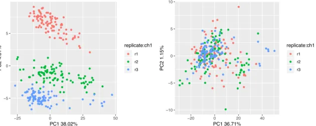
Figure 2.9. PCA before and after ComBat batch correction. The three replicates show a clear separation in the log(counts) data (left), which is corrected after running ComBat (right).
The dataset was downloaded and loaded into the SCTK. In order to reduce the effect of genes with low or no expression, cells with less than 1,700 detected genes and genes with average expression in the bottom 50 percent of the dataset were removed using the filtering tab. The three replicates from the NA19239 sample were used for downstream analysis. The resulting filtered data was visualized on the Dimensionality Reduction and Clustering tab. The batch effect resulting from the plate effect was clearly seen in the data from the log(molecules) assay (Figure 2.9, left). ComBat was run on the
● ● ● ● ● ● ● ● ● ● ● ● ● ● ● ● ● ● ● ● ● ● ● ● ● ● ● ● ● ● ● ● ● ● ● ● ● ● ● ●●● ● ●● ● ● ● ● ● ● ● ● ● ● ● ●●●● ● ● ● ● ● ● ● ● ● ● ● ● ● ● ● ● ● ● ● ● ● ● ● ● ● ● ● ● ● ● ● ● ● ● ● ● ● ● ● ● ● ● ● ● ● ● ● ● ● ● ● ● ● ● ● ● ● ● ● ● ● ● ● ● ● ● ● ● ● ● ● ● ● ● ● ● ● ● ● ● ● ● ● ● ● ● ● ● ● ● ● ● ● ● ● ● ● ● ● ● ● ● ● ● ● ● ● ● ●● ● ● ● ● ● ● ● ● ● ● ● ● ● ● ● ● ● ● ● ● ● ● ● ● ●●● ● ● ● ● ● ● ● ●● ● ● ● ● ● ● ● ●● ● ● ● ● ● ● ● ● ● ● ● ● ● ● ● ● ● ● ● ● ● ● ● ● ● ● ● ● ● ● ● ● ● ● ● ● ● ● ● ● ● ● ● ●● ● ● ● ● ● ● ● ● ● ●● ● ● ● ● ●● ● ● ● ● ● ● ● ● ● ● ● −5 0 5 −25 0 25 50 PC1 38.02% PC2 4.81% replicate:ch1 ● ● ● r1 r2 r3 ● ● ● ● ● ● ● ● ● ● ● ● ● ● ● ● ● ● ● ● ● ● ● ● ● ● ● ● ● ● ● ● ● ● ● ● ● ● ● ● ● ● ● ● ● ● ● ● ● ● ● ● ● ● ● ● ● ● ● ● ● ● ● ● ● ● ● ● ● ● ● ● ● ● ● ● ● ● ● ● ● ● ● ● ● ● ● ● ● ● ● ● ● ● ● ● ● ● ● ● ● ● ● ● ● ● ● ● ● ● ● ● ● ● ● ● ● ● ● ● ● ● ● ● ● ● ● ● ● ● ● ● ● ● ● ● ● ● ● ● ● ● ● ● ● ● ● ● ● ● ● ● ● ● ● ● ● ● ● ● ● ● ● ● ● ● ● ● ● ● ● ● ● ● ● ● ● ● ● ● ● ● ● ● ● ● ● ● ● ● ● ● ● ● ●● ● ● ● ● ● ● ● ● ● ● ● ● ●● ● ● ● ●● ● ● ● ● ● ● ● ● ● ● ● ● ● ● ● ● ● ● ● ● ● ● ● ● ● ● ● ● ● ● ● ● ● ● ● ● ● ● ● ● ● ● ● ● ● ● ● ● ● ● ● ● ● ● ● ● ● ● ● ● ● ● ● ● ● ● ● ● ● ● ● ● ● −10 −5 0 5 10 −20 0 20 40 PC1 36.71% PC2 1.15% replicate:ch1 ● ● ● r1 r2 r3
log(molecules) assay using default parameters (replicate as batch condition, no additional covariates, parametric combat) and saved in an assay named “combat”. The
Dimensionality Reduction and clustering tab was then used to visualize a PCA of the combat assay (Figure 2.9, right). After ComBat, the plates display no signs of batch effects in the first two principal components, indicating that the technical plate artifact has been removed.
The ComBatSCE() function can be used to perform ComBat batch correction on a
SCTKExperiment object. Batch effects can be visualized using reduced dimension data, using functions such as plotPCA() and plotTSNE(). To perform this analysis on the R
console, first the data must be loaded and subset to contain the NA19239 samples only.
R> library(GEOquery)
R> #download data from GEO
R> GSE77288 <- getGEO('GSE77288', GSEMatrix=TRUE) R> con <- gzcon(url(paste(
+ "ftp://ftp.ncbi.nlm.nih.gov/geo/series/GSE77nnn", + "GSE77288/suppl",
+ "GSE77288_molecules-raw-single-per-sample.txt.gz", sep="/"))) R> txt <- readLines(con)
R> dat <- read.table(textConnection(txt), sep = "\t", header=T) R> #extract annotation data from the GSE record
R> pdatasub <- pData(GSE77288$GSE77288_series_matrix.txt.gz)[ + pData(GSE77288$GSE77288_series_matrix.txt.gz)$title %in% + paste(as.character(dat[,1]), as.character(dat[,2]),
+ as.character(dat[,3]), sep="-"),] R> rownames(pdatasub) <- pdatasub$title
R> #transform the count matrix R> datsub <- t(dat[, 4:ncol(dat)])
R> colnames(datsub) <- paste(as.character(dat[,1]), + as.character(dat[,2]),
+ as.character(dat[,3]), sep="-") R> #create SCtkExperiment object
R> GSE77288_sce <- createSCE(assayFile = datsub, + annotFile = pdatasub, + inputDataFrames = T) R> #subset data to NA19239 only
R> GSE77288_sce <- GSE77288_sce[ ,
+ colData(GSE77288_sce)[,"individual:ch1"] == "NA19239"] R> #remove genes with no expression across all cellss
R> GSE77288_sce <- GSE77288_sce[
+ rowSums(assay(GSE77288_sce, "counts")) != 0, ] R> #log transform the count matrix
R> assay(GSE77288_sce, "logcounts") <- log2(assay(GSE77288_sce) + 1) R> #plot before combat
R> plotPCA(GSE77288_sce, useAssay = "logcounts", runPCA = T, + colorBy = 'replicate:ch1')
R> #run combat
+ batch = "replicate:ch1") R> #plot after combat
R> plotPCA(GSE77288_sce, useAssay = "combat", runPCA = T, + colorBy = 'replicate:ch1')
Discussion
We have developed the Single Cell Toolkit (SCTK), a framework for analyzing and visualizing scRNA-Seq data interactively in R. With this toolkit users can process data, visualize the results, and save the data into a convenient object for further
downstream analysis. Because the SCTK uses the SCTKExperiment object, the resulting data object is compatible with other tools that accept SummarizedExperiment or
SingleCellExperiment objects. The toolkit supports various use cases from a user who just wants to visualize preprocessed analysis stored in a data object to a user who wants to perform a full scRNA-Seq pipeline from filtering to pathway activity analysis. The SCTK is the first fully interactive toolkit that allows a user to perform a standard scRNA-Seq workflow from uploading a count matrix to differential expression and pathway activity analysis without writing any code.
Additionally, we have used the analysis workflow available in the SCTK to identify pathway activity differences between breast cancer cells before and after drug treatment. By performing pathway activity analysis on this dataset, we found significant increases in receptor tyrosine kinase (RTK) and epithelial to mesenchymal transition (EMT) pathways, indicating the SCTK can be used to identify biologically meaningful results. (Brady et al., 2017).