2012
Statistical analysis of RNA-seq data from
next-generation sequencing technology
Yaqing Si
Iowa State University
Follow this and additional works at:
https://lib.dr.iastate.edu/etd
Part of the
Bioinformatics Commons,
Biostatistics Commons, and the
Genetics Commons
This Dissertation is brought to you for free and open access by the Iowa State University Capstones, Theses and Dissertations at Iowa State University Digital Repository. It has been accepted for inclusion in Graduate Theses and Dissertations by an authorized administrator of Iowa State University Digital Repository. For more information, please [email protected].
Recommended Citation
Si, Yaqing, "Statistical analysis of RNA-seq data from next-generation sequencing technology" (2012).Graduate Theses and Dissertations. 12682.
by
Yaqing Si
A dissertation submitted to the graduate faculty in partial fulfillment of the requirements for the degree of
DOCTOR OF PHILOSOPHY
Major: Statistics
Program of Study Committee: Peng Liu, Major Professor
Song X. Chen Susan J. Lamont Daniel S. Nettleton Stephen B. Vardeman
Iowa State University Ames, Iowa
2012
DEDICATION
TABLE OF CONTENTS
LIST OF TABLES . . . vi
LIST OF FIGURES . . . vii
ACKNOWLEDGEMENTS . . . ix
ABSTRACT . . . x
CHAPTER 1. General Introduction . . . 1
1.1 Next-Generation Sequencing Technology and RNA-seq Data . . . 1
1.2 Detecting Differentially Expressed Genes . . . 4
1.3 Alternative Splicing . . . 5
1.4 Cluster Analysis . . . 6
1.5 Dissertation Organization . . . 7
CHAPTER 2. An Optimal Test with Maximum Average Power While Con-trolling FDR with Application to RNA-seq Data . . . 8
2.1 Introduction . . . 9
2.2 Method . . . 12
2.2.1 Poisson Model . . . 12
2.2.2 Hypotheses . . . 13
2.2.3 Test for the Poisson Model . . . 13
2.2.4 FDR Control . . . 15
2.2.5 Approximation ofπ(λ, δ) and the Resulting AMAP Test . . . 16
2.2.6 AMAP Test for the Negative-Binomial Model . . . 18
2.3 Simulation Studies . . . 19
2.3.2 Simulation Results . . . 20
2.4 Real Data Analysis . . . 24
2.5 Discussion . . . 25
2.6 Acknowledgement . . . 26
2.7 APPENDICES . . . 27
2.A.1 Proof of the Optimality of the MAP Test . . . 27
2.A.2 EM Algorithm to Estimate the MGN Distributionπ(λ, δ) . . . 27
2.A.3 Fitting the MGN Distribution to Sultan et al. (2008)’s Data . . . 29
2.A.4 Simulation Results with Different Sample Sizes . . . 30
2.A.5 Simulation Results for FDR Control . . . 30
2.A.6 Normalization . . . 31
2.A.7 Simulation Results on Estimation of Dispersion . . . 32
CHAPTER 3. Statistical Analysis of Alternative Splicing Events . . . 43
3.1 Introduction . . . 44
3.2 Model . . . 46
3.3 Hypotheses . . . 48
3.3.1 Test for Inclusion-Skipping . . . 49
3.3.2 Test for Switch-Like Pattern . . . 50
3.3.3 Test for Fold Changes . . . 50
3.4 The AMAP Test . . . 51
3.5 Computation . . . 52
3.6 Simulation . . . 53
3.7 Real Data Analysis . . . 56
3.8 Discussion . . . 57
3.9 APPENDICES . . . 57
3.A.1 Estimation of Background . . . 57
CHAPTER 4. Model-Based Clustering for RNA-seq Data . . . 59
4.1 Introduction . . . 60
4.2 Model . . . 62
4.2.1 Poisson Distribution . . . 62
4.2.2 Negative Binomial Distribution . . . 63
4.3 Model-Based Clustering . . . 63
4.3.1 Model-Based Clustering with the EM Algorithm (MB-EM) . . . 64
4.3.2 Initialization . . . 66
4.3.3 Other Algorithms for Model-Based Clustering . . . 67
4.3.4 Model-Based Hybrid-Hierarchical Clustering Algorithm (MB-HH) . . . 68
4.4 Simulation Study . . . 69
4.4.1 Data simulation . . . 69
4.4.2 Assessment of performance . . . 70
4.4.3 Validation of Estimating Dispersion Parameters . . . 71
4.4.4 Comparison of Initialization Algorithms . . . 73
4.4.5 Comparison of Our Proposed Algorithms with Others . . . 74
4.5 Real Data Analysis . . . 76
4.6 Conclusion . . . 78
4.7 APPENDICES . . . 79
4.A.1 Clustering Results for Simulation . . . 79
4.A.2 Clustering Results for Real Data Analysis . . . 83
CHAPTER 5. General Discussion . . . 87
LIST OF TABLES
1.1 A snapshot of a real RNA-seq data set . . . 3
2.1 Hyperparameters as inputs for simulations . . . 30
2.2 FDR control with the AMAP method . . . 31
LIST OF FIGURES
1.1 The schematic procedures to obtain RNA-seq data . . . 2
1.2 Alternative splicing . . . 5
2.1 Results from testing for DE genes . . . 33
2.2 Comparison of the tests in presense of outliers . . . 34
2.3 Results from testing forF C >1.5 . . . 35
2.4 Analysis of real data from Li et al. (2010) . . . 36
2.5 Analysis of real RNA-seq data . . . 37
2.6 Simulation results for sample sizen= 2,3,5 . . . 38
2.7 FDR control when testing for DE genes . . . 39
2.8 Different normalization methods applied to the AMAP test . . . 40
2.9 Check dispersion estimation for simulation B . . . 41
2.10 Check dispersion estimation for simulation C . . . 42
3.1 Exon effects . . . 47
3.2 Test for expressed exons . . . 55
3.3 Test for switch-like patterns . . . 55
3.4 Test for differential exon usages . . . 56
4.1 Estimation of dispersion parameters . . . 72
4.2 Evaluate initialization of cluster centers . . . 73
4.3 Results of 7 clusters from different clustering methods . . . 74
4.4 Results of 10 clusters from different clustering methods . . . 75
4.6 Clustering results for the maize data set . . . 78
4.7 Estimation of dispersion parameters . . . 80
4.8 Evaluate initialization of cluster centers . . . 81
4.9 Results of seven clusters from different clustering methods . . . 82
4.10 Results of ten clusters from different clustering methods . . . 83
4.11 Clustering real data withK = 20 . . . 84
4.12 Clustering results for the maize data set . . . 85
ACKNOWLEDGEMENTS
I would like to take this opportunity to express my thanks to those who helped me with various aspects of conducting research and the writing of this thesis. First and foremost, Dr. Peng Liu for her guidance, patience and support throughout this research and the writing of this thesis. Her insights and words of encouragement have often inspired me and renewed my hopes for completing my graduate education. I would also like to thank my committee members for their efforts and contributions to this work: Dr. Song X. Chen, Dr. Susan J. Lamont, Dr. Daniel S. Nettleton and Dr. Stephen B. Vardeman.
ABSTRACT
In recent years, the advent of next-generation sequencing (NGS) technology has been revo-lutionizing how genomic studies are processed. One important application of NGS technology is the study of transcriptome through sequencing of RNAs (RNA-seq). Compared with previous technologies such as microarray, RNA-seq data have many advantages, such as providing digital rather than analog signals of expression levels, dynamic and wider ranges of measurements, less noise, higher throughput, etc. Hence, RNA-seq is gradually replacing the array-based approach as the major platform in transcriptome studies. Meanwhile, the massive amounts of discrete data generated by the NGS technology call for effective methods of statistical analysis. There are many interesting questions in RNA-seq data analysis, and we focus on three important ones in this dissertation: identifying differentially expressed genes, from two-treatment experi-ments, detecting alternative splicing patterns using exon-expression data, and clustering gene expression profiles for multi-sample studies. Our major work are introduced in the following chapters:
First, we propose an approximated maximum-average powerful (AMAP) testing procedure to compare gene expression from two treatment groups. The proposed method allows for testing null hypotheses that are much more general than what have been considered by most previous studies, and it leads to a natural way of controlling the FDR. We show that our method has higher power as well as better FDR control than other widely-used methods in practice.
Second, we generalize the AMAP test from testing gene expression data to studying alter-native splicing events from exon-level expression data. A nonparametric algorithm to estimate the distribution of exon usages is proposed, and this algorithm provides more flexibility for fitting the data, and higher computation efficiency. Our method is compared with previous methods and ours is shown to be much more powerful.
models for RNA-seq data, with well-designed initialization strategy and grouping algorithms. We also present a model-based hybrid-hierarchical clustering method to generate a tree struc-ture that allows visualization of relationships among clusters as well as flexibility of choosing the number of clusters. Results from both simulation studies and analysis of a maize RNA-seq data set show that our proposed methods provide better clustering results than alternative methods that are not based on probability models.
CHAPTER 1. General Introduction
1.1 Next-Generation Sequencing Technology and RNA-seq Data
The recent advent of next-generation sequencing (NGS) technology has revolutionized ge-nomic studies. One important application of NGS technology is to study transcriptome through
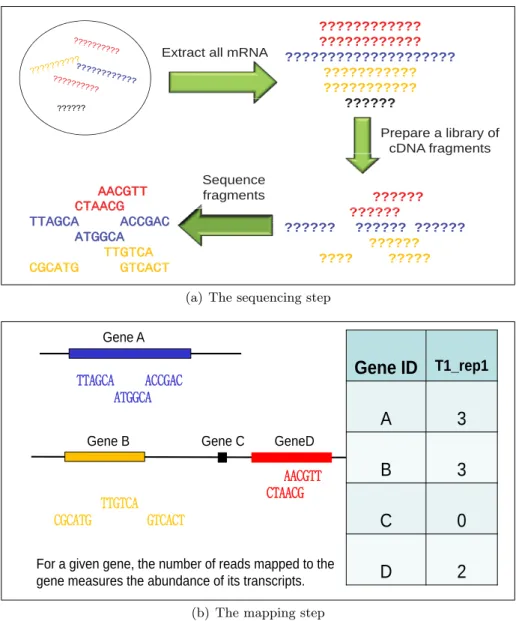
sequencing of RNAs (RNA-seq). In a typical RNA-seq experiment, as shown in Figure 1.1, a
sample of RNA is converted to a library of complementary DNA (cDNA) fragments and then se-quenced on a high-throughput sequencing platform, such as Illumina Genome Analyzer, SOLiD
or Roche 454 (Shendure and Ji, 2008). Millions of short sequences, or namely the reads, are
obtained from this sequencing and then mapped to a reference genome or transcriptome, then the unmapped reads are usually discarded and mapped reads for each sample are assembled into gene-level, exon-level or transcript-level expression summaries, depending on the aims of the experiment, and the count of reads mapped to a given gene/exon/transcript measures the
expression level for this region of the genome or transcriptome. See Table 1.1 for an example
of a typical RNA-seq data set. In the remainder of thesis, we will use ‘gene’ as a general term
for gene/transcript/exon, except in Chapter 3 which will be specified for studying exon-level
RNA-seq data.
Compared with microarray, which has been the dominant approach of studying gene expres-sion in the last two decades, RNA-seq technology has a wider measurable range of expresexpres-sion levels, less noise, higher throughput, and more information to detect allele-specific expression, novel promoters, and isoforms (Wang, Li and Brutnell, 2010; Oshlack et. al, 2010). For these reasons, RNA-seq is gradually replacing the array-based approach as the major platform in gene expression studies. Meanwhile, the massive amounts of discrete data generated by the NGS technology call for effective methods of statistical analysis. The challenging features of
???????????? ???????????? ???????????? ???????????????????? ??????????? ??????????? ??????
Extract all mRNA
?????? Prepare a library of cDNA fragments ?????? ?????? AACGTT CTAACG g Sequence fragments ?????? ?????? ?????? ?????? ?????? ???? ????? CTAACG TTAGCA ACCGAC ATGGCA TTGTCA CGCATGG GTCACT CGCATG GTCACT
(a) The sequencing step
Map sequences to genome
Gene A12 Gene B Gene C GeneD
TTGTCA CGCATG GTCACT TTAGCA ACCGAC ATGGCA AACGTT CTAACG
Gene ID
T1_rep1A
3
B
3
C
0
D
2
For a given gene, the number of reads mapped to the gene measures the abundance of its transcripts.
(b) The mapping step
Figure 1.1: The schematic procedures to obtain RNA-seq data. (a) The sequencing step: a
sample of mRNA is converted to a library of cDNA fragments and then sequenced on a
high-throughput sequencing platform. Millions of short sequences, or namely thereads, are obtained.
For simplicity, each read has length of 6 nucleotides on the figure, while in reality, the length
varies from 26 to hundreds depending on sequencing platforms (Metzker, 2010). (b) The
mapping step: the reads are mapped to a reference genome, and the mapped reads are counted for each gene to measures its expression level. Figures are adapted from lecture notes prepared by Dr. Peng Liu for Stat 416 class, ISU 2012.
Gene ID Gene Number of Mapped Reads
(Name) Length Treatment 1 Treatment 2
g Lg Ng11 Ng12 Ng13 Ng21 Ng22 Ng23 AC233926.1FG3 233 52 80 60 40 45 59 AC234179.1FG1 84 0 0 3 150 92 318 AF466202.2FG4 120 2 2 1 0 0 0 GRMZM2G0423 1304 177 382 200 10 7 6 GRMZM2G0056 587 1 12 7 20 12 38 · · · ·
Table 1.1: A snapshot of a real RNA-seq data set. The experiment has two treatments and
each treatment has three replicates.
RNA-seq data include but mot limited to the following:
- large number of genes: there are often tens of thousands of genes to be compared si-multaneously, hence researchers are more concerned about the overall performance of the analysis than that of a single gene. For example, we want to detect as many truly differentially expressed genes as possible while controlling multiple testing errors . The huge size of RNA-seq data set also requires intensive computation in analysis. Hence high computing power from both machine hardware and algorithm design are desired.
- discrete data type: RNA-seq data use counts of reads to quantify gene expressions, which are very different from continuous data that are can be conveniently modeled by Gaussian distributions. Though some data transformation technique, for instance, calculating the log-transformed counts, can be used to obtain continuous measurement of gene expres-sions, methods that keep and employ the nature of the count data are still preferred. In this sense, discrete probabilities, such as Poisson (Sultan et al., 2008), hypergeometric (Marioni et al., 2008), negative-binomial (NB) (Robinson and Oshlack, 2010; Anders and Huber, 2010). distributions have proposed to model the counts. However, difficulties often exist in the computation or knowing the properties of statistics based on these distributions.
1.2 Detecting Differentially Expressed Genes
One of the primary objectives for most RNA-seq experiments is to compare the gene ex-pression levels across various treatments. A simple and common RNA-seq study involves two treatments in a randomized complete design , for example, treated versus untreated cells, two different tissues from a mouse, cancer or heathy human beings, etc. In these studies, researchers are particularly interested in detecting gene with differential expressions (DE), i.e., genes whose expression levels differ between the two treatments. Detecting DE genes can also be an impor-tant pre-step for subsequent studies, such as clustering gene expression profiles or testing gene set enrichments.
Several methods have been proposed for detecting DE genes based on RNA-seq data.
Among them, Fisher’s exact test (Bloom et al., 2009), χ2 goodness-of-fit test (Marioni et al.,
2008), likelihood ratio test (LRT) (Bullard et al., 2010) and the PoissonSeq procedure (Li et al., 2011) are based on Poisson models for the count data, mostly from RNA-seq experiments that use only technical replicates. However, when there are biological replicates, RNA-seq data may exhibit more variability than what the Poisson distribution predicts, and then the negative binomial (NB) distribution has been used to model the counts in such cases. Based on NB models, several tests have been developed and implemented in the R packages, for instance,
edgeR(Robinson and Smyth, 2008),DESeq(Anders and Huber, 2010) and baySeq(Hardcastle and Kelly, 2010), etc.
Although the above-mentioned methods have been proposed to detect DE genes, there are no theoretical justifications for whether any of these methods are optimal or how to search for the optimal test. Furthermore, most proposed tests are designed for testing whether the mean expression levels are exactly the same or not across treatments, whereas, sometimes, biolo-gists are interested in detecting genes with expression changes larger than a certain threshold. Another issue with current methods is that the multiple testing errors are not well studied. Currently widely-used procedures, include those proposed by Benjamini and Hochberg (1995) and Storey and Tibshirani (2003) for testing methods that generate p-values, are often found to control the false discovery rate (FDR) either conservatively or literally (Li et al., 2011; Kvam
Figure 1.2: Alternative splicing. Two isoforms from one gene: exon 4 is skipped to produce protein A, and exon 3 is skipped for protein B. Figure is from http://images.nigms.nih.gov.
et al., 2012). Hence a new and better performing method of testing for DE genes is in high demand.
We propose an approximated maximum-average powerful (AMAP) testing methods to com-pare gene expressions from two treatment groups. The proposed method allows for testing null hypotheses that are much more general than what have been considered by most previous studies, and it leads to a natural way of controlling the FDR. We show that our method has higher power as well as better FDR control than other widely-used methods in practice.
1.3 Alternative Splicing
For eukaryotic cells, it is common that a gene has several protein-coding regions called
exons, and the exons of a gene are reconnected in multiple ways during RNA splicing. The
resulting different mRNAs are translated into different protein isoforms (see Figure1.2for the
illustration). This process is calledalternative splicing (AS). AS affects message stability and
in particular is known to affect more than half of all human genes, and has been proposed as a primary driver of the evolution of phenotypic complexity in mammals (Lander et al., 2001; Johnson et al., 2003). So studying AS events has been an important question for scientists.
With RNA-seq data, AS can be studied by comparing the coverages of the exons from
different treatments. Though some techniques as introduced in section1.2to detect differential
gene expressions can also be used in comparing exon coverages, specific tools to analyze exon
coverages are still very limited to our best knowledge. Some available methods such likeDEXSeq
(Anders et al., 2012) and MATS (Shen et al., 2012) have been developed to test for differential
exon usages. However, the detection power of these tests has not been evaluated very well.
Moreover, some other interesting AS patterns still need more investigation. For example,
biologists are often interested in testing for expressed exons, or the extreme ‘switch-like’ pattern,
which means that the exon is expressed in one treatment but not in another (see Figure 1.2
where exon 3 is only expressed in the first treatment to produce protein A). All these indicate that studying AS is challenging as well as full of opportunities for statisticians.
We generalize the AMAP test from testing gene expression data to studying alternative splicing events from exon-level expressions. A nonparametric algorithm to estimate the distri-bution of exon usages is proposed, and this algorithm provides more flexibility for fitting the data, and higher efficiency of computation. Our methods is compared with previous methods and is shown to be much more powerful.
1.4 Cluster Analysis
Some RNA-seq experiments involve more than two treatment groups. For example, Li et al. (2010) measured the gene expressions from four representative sections of a leaf blade from a corn plant. By surveying the gene expression profiles along different developmental stages of the leaf, the transcriptional network associated with the development of C4 photosynthesis can be understood. Similar to in microarray studies, in these sequencing experiments with multiple treatment groups, cluster analysis groups genes with similar expression patterns across the treatments. And because genes within such groups often tend to be functionally related, cluster analysis has been employed as an important technique to provide insight into gene functions
and networks.
Many heuristic algorithms, such as K-means and self-organizing map (SOM) (Xiao et al., 2003), have been popularly applied to microarray analysis, and they can potentially be applied to RNA-seq data indirectly, for example, to log-transformed or Z-scores of RPKM of the read counts. However, studies of clustering algorithms with microarray data already revealed that heuristic algorithms usually perform worse than model-based algorithms (Yeung et al, 2001). Hence it is desirable to develop a clustering algorithm based on appropriate probability models specially for RNA-seq data and enhance the performance.
We introduce clustering algorithms based on appropriate probability models for RNA-seq data, with well-designed initialization strategy and grouping algorithms. We also present a model-based hybrid-hierarchical clustering method to generate a tree structure that allows visualization of relationships among clusters as well as flexibility of choosing the number of clusters. Results from both simulation studies and analysis of a maize RNA-seq data set show that our proposed methods provide better clustering results than alternative methods that are not based on probability models.
1.5 Dissertation Organization
The main chapters of this dissertation focus on the three questions introduced in section
1.2, 1.3 and 1.4: In Chapter 2, we present the AMAP test to compare gene expression levels
from two treatment groups; In Chapter3, the AMAP test is generalized to studying alternative
splicing events from exon-level expression data; the model-based clustering method for
RNA-seq data is introduced in Chapter 4. A summary about our work and possible directions for
CHAPTER 2. An Optimal Test with Maximum Average Power While Controlling FDR with Application to RNA-seq Data
Yaqing Si and Peng Liu
Iowa State University, Snedecor Hall, Ames, IA 50011, USA.
This work was submitted toBiometrics
Abstract
The recent RNA-seq technology is an attractive method to study gene expression. One of the most important goals in RNA-seq data analysis is to detect genes differentially expressed across treatments. Although several statistical methods have been published, there are no theoretical justifications for whether these methods are optimal or how to search for the optimal test. Furthermore, most proposed tests are designed for testing whether the mean expression levels are exactly the same or not across treatments, whereas, sometimes, biologists are interested in detecting genes with expression changes larger than a certain threshold. Another issue with current methods is that the false discovery rate (FDR) control is not well studied. In this manuscript, we proposed a test to address all above issues. Under model assumptions, we derive an optimal test that achieves the maximum of average power among those that control FDR at the same level. We also provide an approximated version, the approximated most
average powerful (AMAP) test, for practical implementation. The proposed method allows for
testing null hypotheses that are much more general than what have been considered by most previous studies, and it leads to a natural way of controlling the FDR. Through simulation studies, we show that our test has higher power than other methods, including the widely-used edgeR, DESeq, and baySeq methods, as well as better FDR control than two other FDR control
procedures commonly used in practice. For demonstration, we also apply the proposed method to a real RNA-seq dataset obtained from maize.
Key Words: Empirical Bayes; FDR control; Gene expression; Maximum average power;
RNA-seq.
2.1 Introduction
The recent advent of next-generation sequencing (NGS) technology has revolutionized ge-nomic studies. One important application of NGS technology is the study of the transcrip-tome through sequencing of RNAs (RNA-seq). In a typical RNA-seq experiment, a sample of RNA is converted to a library of complementary DNA fragments and then sequenced on a high-throughput sequencing platform, such as Illumina’s Genome Analyzer. Millions of short
sequences, orreads, are obtained from this sequencing and then mapped to a reference genome.
The count of reads mapped to a given gene measures the expression level of this gene. In the last two decades, microarray technology has been the dominant approach of studying gene expression. Compared with microarray, RNA-seq technology has a wider measurable range of expression levels, less noise, higher throughput, and more information to detect allele-specific expression, novel promoters, and isoforms (Wang, Li and Brutnell, 2010; Oshlack et. al, 2010). For these reasons, RNA-seq is gradually replacing the array-based approach as the major plat-form in gene expression studies. Meanwhile, the massive amounts of discrete data generated by the NGS technology call for effective methods of statistical analysis. For statistical analysis of RNA-seq data, detecting differentially expressed (DE) genes across treatments/conditions is essential, and commonly the major goal of the analysis of RNA-seq data. Additionally, de-tecting DE genes can be a pre-step for subsequent studies, such as clustering gene expression profiles or testing gene set enrichments. In this paper, we focus on the question of detecting DE genes from RNA-seq data. The proposed method can also be applied to the analysis of other types of NGS data, for instance, chromatin immunoprecipitation-sequencing (ChIP-seq) data.
Several methods have been proposed for detecting DE genes based on RNA-seq data. Two popular distributions for fitting RNA-seq data are the Poisson and negative binomial (NB)
distributions. Early RNA-seq studies that used only technical replicates reported that Poisson distributions fit well to the counts for the majority of genes (Marioni et al., 2008; Bullard et al.,
2010). Fisher’s exact test (Bloom et al., 2009), χ2 goodness-of-fit test (Marioni et al., 2008),
likelihood ratio test (LRT) (Bullard et al., 2010), and the PoissonSeq procedure (Li et al., 2011) were applied to detect DE genes. However, when there are biological replicates, RNA-seq data may exhibit more variability than what the Poisson distribution predicts, i.e., the variances are likely greater than the means for a considerable number of genes (Anders and Huber, 2010). This phenomenon is called over-dispersion. In such cases, the NB distribution, which allows the variance to exceed the mean, has been used to model the counts. Based on NB models, several tests have been developed and implemented in the R packages edgeR (Robinson and Smyth, 2008), DESeq (Anders and Huber, 2010) and baySeq (Hardcastle and Kelly, 2010).
Because RNA-seq experiments are still expensive, such experiments typically involve only a few samples from each treatment group. However, each experiment measures an enormous number of genes. For example, the number of measured genes is more than 30,000 for human beings (Pickrell et. al, 2010), and more than 50,000 for maize (Li et al., 2010). This results in
the “largep, smalln” problem for detecting DE genes. A few methods have been proposed to
borrow information across genes in order to achieve better performance in the multiple testing procedure. For example, Robinson and Smyth (2007) proposed an estimator for the dispersion parameter in the NB model that shrinks the dispersion parameter for each individual gene toward a common value using the weighted likelihood approach; Anders and Huber (2010) proposed a local regression model of the variance on the mean using all genes, giving a fitted relationship useful for estimating dispersion parameters; Hardcastle and Kelly (2010) proposed the baySeq method, a test with an empirical Bayes approach. All these methods show higher detection power than those that do not share information. However, there is no theoretical justification for the optimality of these existing methods and no discussion on how to search for the optimal test for RNA-seq data.
In addition to the lack of theoretical guidance in deriving the optimal test, the false discovery
rate (FDR) control is not well studied. FDR has been widely applied to multiple testing
available methods, one may control the FDR with the Benjamini and Hochberg’s procedure (Benjamini and Hochberg, 1995) or Storey and Tibshirani’s procedure (Storey and Tibshirani, 2003) after obtaining the p-values from a test. Only a few studies investigated the performance of these methods in the context of RNA-seq data analysis. Simulation studies by Li et al. (2011) suggest that the FDR control of edgeR may be conservative sometimes. Kvam et al. (2012) also showed that applying Benjamini and Hochberg’s procedure to the p-values generated by DESeq or edgeR was conservative in some cases while liberal in some other cases. Our simulation results
support the same conclusion (see Figure 2.7). Because FDR control directly affects the final
list of DE genes declared by the tests, a good FDR control procedure is highly desired. Moreover, most existing tests are designed for testing the null hypothesis that the difference between expression levels of different treatments is exactly zero for each gene. However, a slight change in the mean expression levels may not be biologically significant. Sometimes, it is more valuable to detect genes with big changes in the mean expressions (MacCarthy and Smyth, 2009; Peart et. al, 2005; Covshoff et al., 2008). A common strategy is to select a list of genes with both high statistical significance and large fold-changes (FC) of expressions between treatments without further evaluation of the FDR of the resulting list (Peart et. al, 2005; Covshoff et al., 2008).
In this paper, we develop an optimal test for RNA-seq data analysis while controlling the FDR, where the optimality is defined as achieving the maximum of the power averaged across all genes for which null hypotheses are false. We call such test the maximum average power (MAP) test, a concept introduced in Chen et al. (2007) and further studied in Hwang and Liu (2010) for microarray data analysis. The statistic of the proposed test provides a natural way of controlling the FDR. Furthermore, the null hypothesis flexibly adapts to the context of problem. The MAP tests are derived for both Poisson and NB distributed data, respectively, where the parameters of these distributions are assumed to come from appropriate hyper distributions. In practice, we do not know the “true” hyper distributions, and we propose to estimate them with mixture distributions. Plugging in the estimated hyper distribution leads to an approximated MAP (AMAP) test. We perform a variety of simulation studies using the Poisson distribution, NB distribution, and real RNA-seq data. Simulation results show that the AMAP test performs
numerically indistinguishable to the optimal MAP test for Poisson data, and the performance of the AMAP test is close to that of the MAP test for NB data. The AMAP test outperforms Fisher’s exact test, edgeR, DESeq and baySeq in most simulation settings. In addition, the results demonstrate that our method provides accurate estimation of the FDR for both the AMAP test and the other tests.
This article is organized as follows: In section 2.2, we describe the proposed method for the
Poisson model and for the NB model; In section 2.3, we simulate RNA-seq data using Poisson
models, NB models and real data, respectively, under a variety of settings, and we evaluate
the effectiveness of the proposed method and other methods; In section 2.4, we analyze a real
dataset using our proposed methods and some existing methods; Section 2.5 provides some
discussion.
2.2 Method
2.2.1 Poisson Model
Suppose that an RNA-seq dataset hasGgenes. LetXgijdenote the number of reads mapped
to genegfrom replicatejof treatmenti, whereg= 1,· · · , G,i= 1,2,j = 1,· · · , ni, andni≥1
is the number of replicates in treatment groupi. Poisson distributions have previously been used
to model the counts when there are only technical replicates of one biological sample for each
treatment group (Bullard et al., 2010; Marioni et al., 2008). Assuming Xgij ∼ Poisson(λgij),
we model the mean of the Poisson distribution,λgij, as
λgij =Sijλgexp(ρiδg), (2.1)
where λg represents the overall geometric mean expression level of gene g across both
treat-ments; ρ1 = −1/2 and ρ2 = 1/2 so that δg is the log fold change (log-FC) between the two
treatment means; andSij is a normalization factor that adjusts for varying sequencing depths
and potentially other technical effects across the replicates. Several proposed methods nor-malize RNA-seq data by estimating the normalization factor in different ways. For example,
we can estimate Sij by the total number of mappable reads (Mortazavi et al., 2008), the 75th
ratio to a pseudoreference (Anders and Huber, 2010), or a scalar estimated by method of the
trimmed mean of M-values (TMM) (Robinson and Oshlack, 2010). In Appendix 2.A.6, we
revisit this issue and present results with different normalization methods. After estimation,
Sij is usually treated as known in the followup analysis.
2.2.2 Hypotheses
One major goal of RNA-seq experiments is to identify genes whose expression levels change across different treatment groups. To achieve this goal, we test the following hypotheses
re-garding the parameter δg for each geneg:
H0g:δg ∈∆0 v.s. H1g:δg∈∆1, (2.2)
where ∆0 and ∆1 correspond to the null and alternative sets of values forδg, respectively, and
they represent a partition of the real line R. The null space ∆0 can be defined in different
ways depending on the biological questions of interest. For example, we set ∆0 = {0} if we
are interested in knowing whether the mean expression levels in the two treatments are equal. If we are interested in whether the mean expression is higher in the second treatment than in
the first, we set ∆0 = (−∞,0]. Sometimes, biologists want to detect genes whose expression
changes are large enough, for instance, with fold-changes of expressions greater than 1.5 (Peart
et. al, 2005). In this case, we set ∆0 ={δ :|δ| ≤c}withc= log 1.5. The test we derive in the
next section allows for any ∆0 that is a subset of R. Most other tests only allow the simple
null hypothesis ∆0={0}. This is an important advantage of our method over others.
2.2.3 Test for the Poisson Model
Our goal is to derive MAP tests while controlling FDR. As in Storey (2007) and in Hwang and Liu (2010), we focus on the hypothesis rejecting strategy that does not depend on individual genes. Storey (2007) calls such type of testing procedure the single thresholding procedure (STP) and explains that it is often the only available option in practice. Theorem 3 in Hwang and Liu (2010) proves that, for STPs, the MAP test while controlling the average type I error
rate is the MAP test when controlling the FDR. Therefore, we will derive the MAP test by maximizing the average power while controlling the average type I error rate.
Let Xg = {Xgij :i = 1,2;j = 1,· · ·, ni} ∈ X denote the vector of observations for gene
g, where X is the data space that contains all possible values for Xg. Let f(Xg|λg, δg) be
the likelihood function for the Poisson model (2.1), and let ϕ(Xg) be a critical function that
takes the value of 1 or 0 so that the hypothesis H0g is rejected if and only if ϕ(Xg) = 1.
Then, the power for testing gene g is RXϕ(Xg)f(Xg|λg, δg)dXg, and the average power is
1 G1
P
{g:δg∈∆1}
R
Xϕ(Xg)f(Xg|λg, δg)dXg, where G1 is the number of genes with δg ∈ ∆1.
When the (λg, δg)’s forδg ∈∆1 are assumed to be random variables coming from a distribution
with probability density function (PDF)π1(λ, δ) with supportR+×∆1, then as G1 → ∞, the
average power converges to
Z R+ Z ∆1 Z X ϕ(X)f(X|λ, δ)dX π1(λ, δ)dδdλ, which by Fubini’s theorem is equal to Z X ϕ(X) Z R+ Z ∆1 f(X|λ, δ)π1(λ, δ)dδdλ dX. (2.3)
Note that the subscriptgis not needed in this integration. Similarly, if we assume the (λg, δg)’s
of the genes withδg∈∆0 follow a distribution with PDFπ0(λ, δ) with support R+×∆0, then
the average type I error rate of these tests approaches
Z X ϕ(X) Z R+ Z ∆0 f(X|λ, δ)π0(λ, δ)dδdλ dX (2.4) asG0 → ∞, whereG0 =G−G1.
Applying the Neyman-Pearson lemma, we claim that the optimal test that maximizes the
average power (2.3) while controlling the average type I error rate (2.4) rejectsH0g when the
following statistic is small:
T∗(Xg) = R R+ R ∆0f(Xg|λ, δ)π0(λ, δ)dδdλ R R+ R ∆1f(Xg|λ, δ)π1(λ, δ)dδdλ .
See the Appendix for the proof for this claim. If we define a mixture distribution of (λg, δg) by
π(λ, δ) = p0π0(λ, δ) + (1−p0)π1(λ, δ), where p0 is the proportion of genes withδg ∈∆0, and
apply a monotonic transformation of T∗(Xg), we obtain an equivalent test statistic:
T(Xg) = R R+ R ∆0f(Xg|λ, δ)π(λ, δ)dδdλ R R+ R Rf(Xg|λ, δ)π(λ, δ)dδdλ . (2.5)
Applying Theorem 3 of Hwang and Liu (2010), we can also prove that the test that rejectsH0g
when the statistic (2.5) is small also maximizes the average power among the tests that control
FDR at the same level. Now we formally summarize this result in the following theorem:
Theorem 1. Most Average Powerful (MAP) Test. The test that maximizes the average power
(2.3) with FDR controlled at level α is the test that rejects H0g using the rejection region
C={Xg :T(Xg)≤c}
for g = 1,2, ..., G, where the test statistic T(Xg) is defined in (2.5), and the constant c is the critical value so that the multiple testing procedure has FDR controlled at level α.
We call the test with critical function ϕ∗(X) := I(X ∈ C) as described in Theorem 1 an
MAPtest, where I(·) is the indicator function.
2.2.4 FDR Control
In this section, we present how we estimate the FDR level of the MAP test given a critical value for the test statistic. One can control the FDR to the desired level by choosing the appropriate critical value.
Within Bayesian framework, π(λ, δ) can be considered as the prior distribution for (λg, δg).
It is straightforward to show that T(Xg) defined in (2.5) is P(δg ∈ ∆0|Xg), the posterior
probability of δg ∈ ∆0 given the data. Then, for a test with critical function ϕ(Xg), the
expected number of false positives (EFP) can be estimated by P
gT(Xg)ϕ(Xg). Finally the
FDR can be estimated by the ratio of the estimated EFP to the number of rejected hypotheses:
d FDR = P gT(Xg)ϕ(Xg) P gϕ(Xg) , (2.6)
which can be viewed as the average posterior probability of being false positive for the list
of genes declared to be positives by ϕ. Note that the above critical function ϕ(Xg) is not
necessarily for the MAP test ϕ∗, but can be for any test that is an STP. As a result, the FDR
2.2.5 Approximation of π(λ, δ) and the Resulting AMAP Test
The derivation of the MAP test assumes the knowledge of the joint distribution π(λ, δ).
However, in practice, we do not know this distribution and need to estimate it. Considering the high dimensionality of tests, computational efficiency is highly desired. For this reason,
we assumes a parametric model for the distribution of π(λ, δ). In addition, we would like our
model to be flexible enough to provide good fitting for various datasets. The model we propose
forπ(λ, δ) is:
K X
k=1
qkG(λ|αk, βk)N(δ|µk, σk), (2.7)
where K is the number of components of the mixture model;qk is the weight of mixing
com-ponent kwithqk>0 and
PK
k=1qk= 1,G(· |αk, βk) is the PDF of a Gamma distribution that
has mean αk/βk and variance αk/βk2, and N(· |µk, σk) is the PDF of a Normal distribution
with meanµk and varianceσk2. We call the distribution (2.7) aK-componentmixture
Gamma-Normal (MGN) distribution. Note that the Gamma distribution is the conjugate prior for the
Poisson distribution, which will simplify the calculation ofT(Xg) in equation (2.5) by reducing
one dimension of integration. In addition, by varying the number of components, the mixing weights, and the parameters of each component, the mixture distribution provides ample model flexibility.
Given a positive integer K, the unknown hyperparameters parameters inπ(λ, δ) are
θ={(qk, αk, βk, µk, σk) :k= 1,2,· · · , K}.
In Appendix2.A.2, we provide an Expectation-Maximization (EM) algorithm to estimate these
parameters simultaneously. Plugging the estimated π(λ, δ) into the formula for the MAP
statistic T(Xg), we obtain an approximated MAP (AMAP) test. To apply AMAP test in
practice, we also need to determine a proper value forK.
If K = 1, λg and δg are assumed independent by model (2.7). This is not necessarily
appropriate for some RNA-seq data. In addition, the one-component MGN distribution may not be able to provide a good approximation to the true distribution. Considering the mean
expression λ only, the single Gamma distribution often expects fewer highly expressed genes
between λ and δ, a more flexible shape for the MGN distribution, and hence a likely better
approximation of the true distribution. However, a bigger K means more hyperparameters
in π(λ, δ) to estimate as well as more computation to calculate the statistic T(Xg). Thus in
practice, it is not desirable to choose a very largeK.
Our experience with several datasets suggests that K = 3 usually provides a good
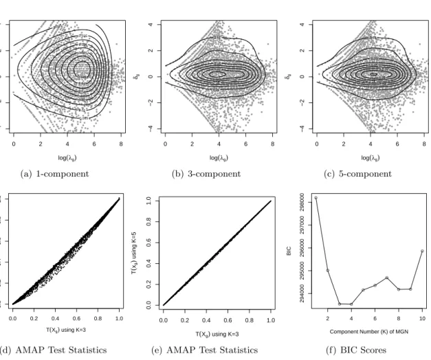
per-formance. To illustrate how to choose K, we show an example of analyzing a real RNA-seq
dataset from Sultan et al. (2008), which studied the transcriptomes from a human embryonic
kidney and a B cell line without biological replicates. See Appendix 2.A.3 for the details of
the analytical results. For this dataset, the model parameters of the MGN distribution for
K = 1,2,· · · ,10 were estimated. From visual inspection of model-fit (Figure 2.5(a)-2.5(c)),
comparison of the values of the AMAP statistics (Figure 2.5(d)-2.5(e)), and the Bayesian
In-formation Criterion (BIC) scores calculated for these MGN-Poisson hierarchical models (Figure
2.5(f)), we found that K= 3 provides the best fit for this dataset.
The model (2.7) without parameter constraints works well when the null space ∆0 consists
of one or several intervals of R. However, if we test for the simple null hypothesis δg = δ0,
it is found that T(Xg) ≡ 0 according to equation (2.5) because of the continuity of
Nor-mal distributions. To solve this problem, we view the δ for the null genes as coming from a
degenerated Normal distribution,N(δ0,0), that has a point mass at δ0. Then, the joint
distri-bution of λand δ for the null genes takes the form of π0(λ, δ0) =π0(λ)N(δ0,0). To estimate
π(λ, δ) = p0π0(λ)N(δ0,0) + (1−p0)π1(λ, δ), we estimate π0(λ) by a K0-component mixture
Gamma distribution andπ1(λ, δ) by aK1-component MGN distribution, whereK0 andK1 are
positive integers. Hence, we approximateπ(λ, δ) by a (K =K0+K1)-component MGN
distri-bution with parameters{(qk, αk, βk, µk, σk) :k= 1,· · ·, K}, among whichK0 components have
known parameters µk = δ0 and σk = 0 for k = 1,· · · , K0. All the unknown parameters can
be estimated by the EM algorithm described in Appendix2.A.2. We found thatK0 =K1= 3
2.2.6 AMAP Test for the Negative-Binomial Model
As mentioned in section 2.1, RNA-seq data with biological replicates often exhibit
over-dispersion while fitting the Poisson model. Assuming an NB instead of a Poisson model is one way to deal with over-dispersed data because the NB distribution specifies that the variance is greater than the mean. Following Robinson and Smyth (2007), we parameterize the variance of the NB distribution by:
Var(Xgij) =λgij+φgλ2gij, (2.8)
where λgij is the mean and is modeling using (2.1), and φg is the dispersion parameter that
determines the extra variability compared to the Poisson model. The variance Var(Xgij)
ap-proaches the mean λgij when the dispersion parameter φg diminishes to 0, thus the Poisson
model can be viewed as a special NB model that has zero dispersion (Robinson and Smyth, 2007).
The NB model defined by equations (2.1&2.8) has three unknown parameters, (λg, δg, φg),
for each gene. Assuming we know their joint distribution, π(λ, δ, φ), the MAP test statistic
takes the following form:
T(Xg) = R R+ R R+ R ∆0f(Xg|λ, δ, φ)π(λ, δ, φ)dδdλdφ R R+ R R+ R Rf(Xg|λ, δ, φ)π(λ, δ, φ)dδdλdφ . (2.9)
Again,π(λ, δ, φ) is unknown in practice. We could generalize the MGN model (2.7) forπ(λ, δ) so
thatπ(λ, δ, φ) is approximated by the mixture modelPKk=1qkG(λ|αk, βk)N(δ|µk, σk)G(φ|ak, bk)
with additional hyperparametersak, bk >0. However, since there is no obvious conjugate prior
for the NB model, the three-dimensional integrations in the calculation of the test statistic
(2.9) and the EM algorithm for estimating the hyperparameters require intensive computation.
Instead of trying to estimate π(λ, δ, φ) and compute the three-dimensional integrations, we
take an approximating approach for the NB model. First, we estimate the dispersion parameter
φg for each gene by the quasi-likelihood (QL) approach. Other methods of estimating φg such
as those discussed in Nelder (2000) and Robinson and Smyth (2008) can also be applied. Then,
the estimateφbgis treated as the trueφgfor geneg. We modelπ(λ, δ) by an MGN distribution as
in Appendix2.A.2. With the estimated distribution, bπ(λ, δ), the AMAP statistic is T(Xg) = R R+ R ∆0f(Xg|λ, δ,φbg)bπ(λ, δ)dδdλ R R+ R Rf(Xg|λ, δ,φbg)bπ(λ, δ)dδdλ , (2.10)
where the likelihood function f(Xg|λ, δ,φbg) is calculated based on the NB model (2.1 &2.8).
The FDR for the AMAP test based on the NB model can also be estimated by equation (2.6).
2.3 Simulation Studies
In this section, we evaluate the proposed tests and some existing methods with three sim-ulation studies. For each simsim-ulation setting, we simulated 50 independent datasets with each
dataset containing 10,000 genes, 2 treatment groups andnreplicates for each treatment group
wheren varied between 2, 3, 5 and 10.
2.3.1 Data Simulation
Simulation A: Poisson Model-Based
. For this simulation, data were simulated from independent Poisson distributions. First,
we estimated the distribution of π(λ, δ) for the RNA-seq dataset analyzed in Sultan et al.
(2008) by fitting a 3-component MGN distribution (see section 2.2.5). Given the estimated
parameters {(qk, αk, βk, µk, σk) : k = 1,· · · ,3} (see Table 2.1), we drew λg and δg from the
MGN distribution independently. Then, p0 ×100 % of the genes were randomly chosen and
their δg values were set to be zero. Finally, the λgij was calculated based on equation (2.1),
where the normalizing factorsSij for alliand j were set to be 1, and thenNgij was generated
from the Poisson(λgij) distribution.
Simulation B: Negative-Binomial Model-Based
. The mean expression level λgij was generated in the same way as in Simulation A. The
dispersion parameters φg were independently drawn from a Gamma distribution with mean
α/β = .85/2 and variance α/β2 = .85/22, following the simulations of Hardcastle and Kelly
(2010). Then the countNgij was drawn from a NB distribution with meanλgij and dispersion
Simulation C: Real Data-Based
. This simulation was based on a large population-based RNA-seq experiment that se-quenced 69 lymphoblastoid cell lines (LCL) derived from unrelated Nigerian individuals (Pick-rell et. al, 2010). The samples were sequenced at two separate labs (Argonne and Yale) on Illumina Genome Analyzer II instruments, but the two labs generated reads with different lengths. We only selected one lane for each individual from those sequenced at Yale. For
each simulation we randomly selected 2n out of the 69 individuals and randomly assigned n
to one hypothetical treatment group and the remaining n samples to the other hypothetical
treatment group. Then, 10,000 genes were randomly selected after excluding those with zero counts across all individuals in both treatments. We expect no differential expression for these genes because the samples were randomly picked from the same population. Then a random
sample of (1−p0)×100% of the selected genes were set to be DE, and their counts in the first
and second treatment group were multiplied by exp(−δg/2) and exp(δg/2), respectively, where
δg was drawn from a N(0,1) distribution. The scaled numbers were rounded to the nearest
integers. This simulation setting is expected to best mimic the real data because all the counts were originated from real data and no distributional assumptions were imposed.
2.3.2 Simulation Results
2.3.2.1 Testing for Differential Expression
We test the null hypothesis δg = 0 for each gene, which will be referred to as testing for
differential expression (DE). For each dataset, we estimated the distribution, π(λ, δ), by the
method described in section 2.2.5, and calculated the AMAP statistics with the estimated
distribution. We used the Poisson likelihood for simulation A and the NB likelihood for sim-ulations B and C to calculate the AMAP statistics. Fisher’s exact test, edgeR, DESeq and baySeq were also applied to each dataset for comparison. To evaluate the test performance without the influence of different normalization methods, we use the same normalization factors for all tests except Fisher’s exact test. Specifically, we set all normalization factors to be 1 for
treatment ibefore modifying the counts to generate DE genes.
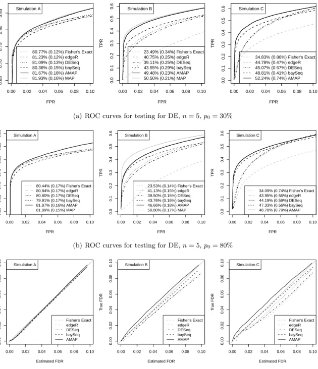
Receiver Operating Characteristic (ROC) curves that plot the true positive rate (TPR)
versus the false positive rate (FPR) are shown in Figures 2.1(a) and 2.1(b) for results with
n = 5. ROC curves for different tests when n= 2,3, and 10 are shown in Figure 2.6. These
curves are results of averaging over 50 datasets. We plotted the curves over the FPR values between 0 and 0.1 because the range of small FPR values are of the most practical importance. In addition, we calculated the area under the curve (AUC) for the same range of FPR. The average values and standard errors of the AUC from the 50 simulated datasets are reported in the figure legends. The AUC values presented in all figures are the percentages of 0.1, where 0.1 is the total area for the plotted range of FPR.
For simulations A and B, we also calculated the MAP statistics by equation (2.5) with the
true distribution of π(λ, δ) used to simulate data. Although this is not available in practice,
based on the derivation in section2.2, the MAP test should provide the highest average power,
and hence it is also included for the evaluation of other tests.
Figures2.1(a)and2.1(b)shows that the MAP test indeed generated the highest ROC curve
and largest AUC among all tests as we expected. We also find that the ROC curves of the AMAP and MAP tests are almost identical for simulation A, and are close for simulation B. The performances of Fisher’s exact test, edgeR, DESeq and baySeq are comparable for simulation A, with edgeR and DESeq being slightly better. For simulation B, Fisher’s exact test performs much worse than the others, and the baySeq method is the best among edgeR, DESeq and baySeq. In both simulations A and B, the AMAP test significantly outperforms all these tests. For simulation C, the MAP test is not included in the comparison because we do not know
the true distribution π(λ, δ). The performance of the AMAP test is superior to that of the
other tests. For small values of FPR, the improvement of average power is dramatic. When the FPR is 0.01, the TPR for the AMAP test almost doubles the TPR for edgeR and DESeq
(Figure 2.1(a)). Because this simulation setting does not depend on parametric assumptions
but is based on real RNA-seq data, the results show that the AMAP test is robust to our model assumptions and can be expected to provide better rankings of genes compared with the other tests when applied to real data.
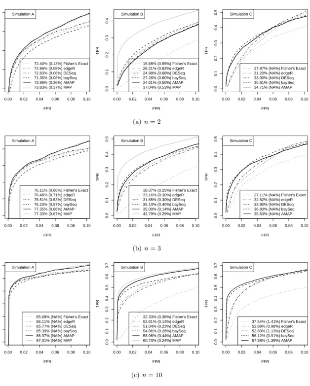
In Appendix 2.A.4, we present more simulation results with varying sample sizesn= 2,3,
and 10 (Figure2.6). For simulation A, the performance of AMAP test is indistinguishable from
the MAP test for all sample sizes, and both the MAP and AMAP tests are superior than the
other tests. For simulation B and C, the AMAP is outperformed when n= 2 (Figure 2.6(a)).
When n = 3, AMAP and baySeq have similar performance that is better than other tests
(Figure2.6(b)). Whenn= 10, AMAP is clearly better than all other tests (Figure 2.6(c)) as
shown here when n= 5 (Figure 2.1).
We also estimated the FDR for all tests using the AMAP test statistics and equation (2.6)
as described in section2.2.4. The true proportion of false positives among all declared positives
at each level of the estimated FDR was plotted in Figures2.1(c). The estimated FDR levels by
our proposed method for all these tests are almost identical to the true values for simulation A. For simulations B and C, the estimated FDR levels are very close to the true values but with
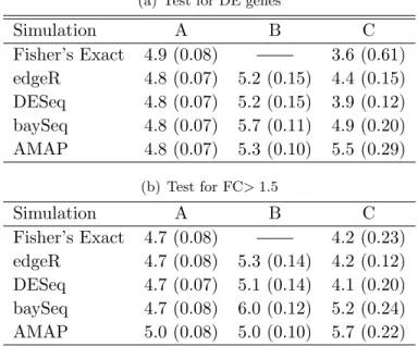
slight underestimation. Table 2.1(a) presents the average proportions of false positives (true
FDRs) and standard errors for all tests when we control the FDR level at 5% using our proposed method. The true FDRs are between 3.6% and 4.9% for simulations A and C except for one that is 5.5%, and they range from 5.2% to 5.7% for simulation B. For comparison, other widely-used FDR controlling procedures proposed by Benjamini and Hochberg (1995) and Storey and Tibshirani (2003) were also applied to the p-values produced by Fisher’s exact test, edgeR and DESeq. The two procedures were not applied to baySeq because baySeq does not provide p-values. In contrast to the good estimation of FDR using the AMAP test statistics, neither of
these two procedures controlled the FDR satisfactorily in any of the simulations (Figure 2.7).
Combining the results for the ROC curves and FDR control, we conclude that the proposed AMAP tests generate better rankings of genes in most simulation settings and provide accurate estimation for FDR, and hence provide more reliable lists of DE genes at a desired level of FDR control.
2.3.2.2 Simulation with Outliers
Li and Tibshirani (2011) showed that in real data, there exist outliers that are not well modeled with the negative binomial model. To check the effect of outliers on the performance
of the AMAP test, we modified simulation B (with n = 5 and p0 = 80%) according to the
simulation conducted in section 3.2 of Li and Tibshirani (2011). Specifically, after λgij was
simulated, we randomly sampled 1% of these λgij and setλgij ←10λgij.
Comparing the results for data with outliers (Figure2.2) with the results for data without
outliers (the middle panel of Figure 2.1(b)), the MAP test assuming no outliers clearly suffer
a lot by the introduction of outliers as the AUC drops from 50.8% to 35.4%. The AUCs of all the other tests, edgeR, DESeq, baySeq and Fisher’s exact test, are dramatically decreased too. However, the AMAP test is only modestly affected, with AUC dropping from 46.66% to 44.05%. As a consequence, the results show that AMAP test is superior than all the other
tests when there exist outliers (Figure 2.2). Again, this show that while the MAP test is only
optimal under the model assumptions, the AMAP test is pretty robust and performs well even the model assumptions are violated.
2.3.2.3 Testing for Fold-Changes
Sometimes, biologists want to detect genes whose expression change between treatment groups is large enough (MacCarthy and Smyth, 2009; Covshoff et al., 2008). A common practice
is to apply a two-step procedure. The first step is to select a list of DE genes by testingδg= 0
while controlling FDR at a certain level. The second step is to select the genes that have large
enough fold-changes (FC), such as FC>1.5, among the list of DE genes identified in the first
step. The FC can be estimated by the ratios of the mean normalized counts between the two treatments groups. However, the power of such a procedure is not well studied, and oftentimes, the FDR is not estimated for the list of genes detected by this procedure.
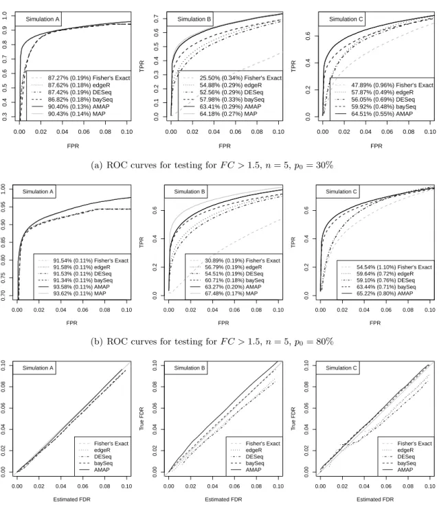
Within the framework introduced in section 2.2, we can apply the MAP test and the
AMAP test for the null hypothesisδg∈∆0 where ∆0 ={δ :|δ| ≤log(F C)}in order to detect
interesting genes with the FC exceeding a pre-determined threshold. We call this testing for FC,
which is more general than testing for DE where ∆0 ={0}. Again, the AMAP test statistics
and FDR estimation can be calculated by equation (2.5) and formula (2.6), respectively. The
ROC curves in Figures2.3(a)and 2.3(b)show that the AMAP test performs almost identically
two-step procedure using other tests, especially for the range of small FPR values that is of more
practical interest. Figure 2.3(c)shows that the estimated FDR levels by our proposed method
for all these tests are almost identical to the true values for simulation A. For simulations B and C, the estimated FDR levels are very close to the true values but with slight underestimation.
Table2.1(b)presents the average proportions of false positives (true FDRs) and standard errors
for all tests when we control the FDR level at 5% using the proposed method. The FDR is well controlled for all cases except two where the FDR control is slightly liberal (5.7% and 6%).
Note that we have used the same normalization method for the AMAP, edgeR, DESeq and baySeq tests to obtain all the above simulation results. In real data analysis, we need to
estimate the normalization factor (Sij) to adjust for varying sequencing depths and potentially
other technical effects across replicates. We compared different normalization methods in the
Appendix 2.A.6. When there are symmetric differential expression, the total count method,
the third quartile method (Bullard et al., 2010), and the median method by Anders and Huber
(2010) perform similarly for AMAP test (Figure 2.8). When the differential expression effect
is not symmetric, the total count is worse than the other two normalization methods. In both settings, the AMAP tests with all three normalization methods are superior to DESeq and edgeR test when compared with the default normalization method for associated R packages.
2.4 Real Data Analysis
In this section, we analyze a real RNA-seq dataset published by Li et al. (2010). The dataset can be downloaded from the NCBI short read archive under accession number SRA012297. In this experiment, the maize leaf transcriptome was quantified using Illumina Genome Analyzer II. The dataset includes measurements of transcript abundance of two cell types, bundle sheath and mesophyll, for the tip of maize leaf at a well-defined developmental stage. Each cell type has two biological replicates. In this article, we are interested in comparing the gene expressions between the two cell types.
We assume NB models for the expression counts observed for each gene, and we perform Fisher’s exact test, edgeR, DEseq and baySeq tests, and the AMAP test as described in section
2.3.2.1and2.3.2.3. We also estimated the FDR levels using formula (2.6) for all these tests. The
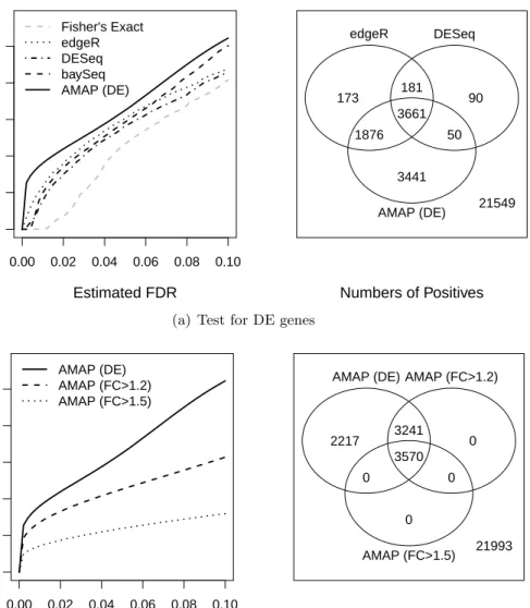
numbers of detected DE genes at different FDR levels are shown in Figure 2.4(a). Among all
testing methods, the AMAP test detected the most DE genes, or equivalently, the estimated FDR level for the AMAP test was the smallest if we declared the same number of positive genes for all applied tests. Moreover, the majority of genes detected by other methods were
also identified by the AMAP test. For example, as shown in Figure 2.4(a), when the FDR is
controlled at 1%, the AMAP test detected 5537 of the 5891 genes detected by edgeR, and in addition, 3491 genes were detected by the AMAP test but not by edgeR. Note that detecting the most DE genes is not necessarily an indicator of the best method. Follow-up experiments to confirm the extra detected genes will help evaluation of the AMAP method.
We also tested for genes that have expression fold changes exceeding a threshold, F C =1.2
or 1.5, by testing hypotheses H0 : |δg| ≤ log(F C) with the AMAP test. Not surprisingly, as
shown in Figure2.4(b), when the threshold increases, less genes are detected, and the positive
genes rejected at a higher threshold are always detected at a lower threshold.
2.5 Discussion
In this article, we provide a framework for finding the optimal test for RNA-seq data, i.e., the one that maximizes the average power while controlling the FDR. We derive the MAP tests under Poisson and NB models, respectively, and also provide the approximation of the optimal tests, AMAP tests, to be applied in practice. The simulation studies show that the proposed methods perform better than edgeR, DESeq, baySeq and Fisher’s exact test. Excluding the proposed methods, baySeq performs better than all other methods. In fact, baySeq can also be viewed as an approximated MAP test where the joint prior distribution is estimated empirically. This helps to explain the near-optimal behavior of the baySeq method.
The results of the AMAP tests are numerically indistinguishable from that of the MAP tests for the Poission model, while the difference between the AMAP and MAP tests is more obvious for the NB model. One reason for this is that there is an extra dispersion parameter in the NB model, and it is challenging to obtain a good estimate or an approximate distribution of this parameter. The estimation of the dispersion parameter for the NB model in the context of
RNA-seq data analysis has drawn attention recently (Robinson and Smyth, 2007; Anders and
Huber, 2010; Hardcastle and Kelly, 2010). In Appendix2.A.7, we compared the performance
of the AMAP tests using three different methods to estimate dispersion parameters: the quasi-likelihood (QL) approach, and the edgeR and DESeq approaches proposed by Robinson and
Smyth (2007) and Anders and Huber (2010), respectively. We found that whenn= 2, the QL
approach is slightly worse than edgeR and but slightly better than DESeq, while whenn= 3,5
and 10, QL method performs better than the other two for simulation B. For simulation C,
the QL approach is better than edgeR and DESeq for all sample sizesn= 2,3,5 and 10. The
AMAP tests with estimated dispersion parameters performs worse than the AMAP test with
true dispersion parameter and the same estimatedπ(λ, δ). This suggests that better estimation
method of the dispersion parameter will likely further improve the performance of the AMAP test.
Although the proposed method is illustrated within the context of RNA-seq data analysis, the AMAP test is also applicable to ChIP-seq data to identify genomic regions of protein
occupancy by testing the null hypothesisδg ∈(−∞,0]. Moreover, the framework shown in this
article gives a general approach to build optimal tests in multiple hypothesis testing problems.
The R package, named AMAP.Seq, is publicly available on http://www.r-project.orgfor
implementation of our methods. Users can choose either Poisson or NB distribution to model the counts and specify their own estimates of the normalization factors or dispersion parameters.
The computation takes about 45 minutes for a typical RNA-seq dataset withG= 10,000 and
n1=n2= 5 using a Windows machine with a 3.4GHz CPU and 8GB RAM.
2.6 Acknowledgement
2.7 APPENDICES
2.A.1 Proof of the Optimality of the MAP Test in Section 2.2.3to Maximize the
Average Power While Controlling the Average Type I Error Rate
In addition to the notations in section2.2, we denotefi(X) =
R
R+ R
∆if(X|λ, δ)πi(λ, δ)dδdλ
for i= 0 or 1. Since R
X fi(X)dX = 1, fi(X) defines the PDF of a distribution for X on X.
Then, the average power (2.3) is equal toRXφ(X)f1(X)dX, and the average type I error rate
(2.4) isR
Xφ(X)f0(X)dX. According to the Neyman-Pearson Lemma, the most powerful test
that maximizes R
Xφ(X)f1(X)dX for each fixed level of
R
Xφ(X)f0(X)dX has a rejection
regionC={X ∈ X :T∗(Xg) =f0(X)/f1(X)≤c} for some critical value c.
2.A.2 EM Algorithm to Estimate the MGN Distribution π(λ, δ)
In section 2.5 in the main manuscript, we approximate the joint distribution π(λ, δ) by a
K-component MGN distribution defined in equation (7). Suppose that we have determined the
number of componentsK forπ(λ, δ), orK0 forπ0(λ, δ) andK1forπ1(λ, δ) withK =K0+K1,
then the parameters in the MGN distribution are
θ={(qk, αk, βk, µk, σk) :k= 1,· · ·, K}.
Using our settings in section 2.5, all parameters except {(µk =δ0, σk= 0) :k= 1,· · ·, K0}
inθ are unknown if the normal components inπ0(λ, δ) are degenerate atδ =δ0; otherwise, all
parameters in θ are unknown. We introduce a vector Zg = (Zg1,· · ·, ZgK) for gene g, where
Zgk is one or zero according to whether (λg, δg) is from componentkof the mixture distribution
or not. Assume that the Zg’s are independent samples from a multinomial distribution that
consists ofK categories with probabilitiesq= (q1,· · ·, qK). The full data from the hierarchical
model are
(X,λ,δ,Z) ={(Xg, λg, δg,Zg) :g= 1,2,· · · , G},
where X = (X1,· · · ,XG) are observed, and (λ,δ,Z) are latent variables. Then the
non-observable variables (λ,δ,Z) and unknown hyperparameters inθcan be estimated via an EM
1. Initialization. First obtain the estimates of λg and δg from the Poisson model using
their maximum likelihood estimates (MLE). Assuming there are no degenerate normal
components inπ(λ, δ), classify the genes intoKgroups by clustering the points (logbλg,bδg)
via the K-means method. Assuming a degenerate normal distribution in π0(λ, δ), force
all bδg’s that are close to δ0, say the ones with |δbg−δ0| < 0.1, to be equal to δ0, then
randomly assign these genes into K0 groups, and cluster all other genes by their values
of (logbλg,δbg) into K1 groups. Then, in both cases, assuming bλg and bδg in group k
are independently from the gamma distribution G(λ|αk, βk) and (degenerate) normal
distributionN(δ|µk, σk), respectively, (αk, βk) and (µk, σk), if unknown, can be estimated
by their MLEs. The weight qk for component k can be initialized by the proportion of
genes in groupk.
2. E-step. With the estimated hyperparameters inθfrom the previous step, the expectations of the latent variables can be calculated. We have
E(Zgk|Xg,θ) =
qkf(Xg|αk, βk, µk, σk) P
lqlf(Xg|αl, βl, µl, σl)
,
where f(Xg|αk, βk, µk, σk) is the density function of the conditional distribution of Xg
given that (λg, δg) are from componentk of π(λ, δ):
f(Xg|αk, βk, µk, σk) =
Z Z
f(Xg|λ, δ)G(λ|αk, βk)N(δ|µk, σk)dλdδ.
Here,f(Xg|λ, δ) is the density function for the Poisson model, and it should be replaced
throughout byf(Xg|λ, δ,φbg) for the NB model after estimating the dispersion parameter
φg. Furthermore, the expectations of λg and δg are
E(λg|Xg,θ) = X k qk Z Z λf(λ, δ|Xg, αk, βk, µk, σk)dλdδ and E(δg|Xg,θ) = X k qk Z Z δf(λ, δ|Xg, αk, βk, µk, σk)dλdδ,
wheref(λ, δ|Xg, αk, βk, µk, σk) is the conditional distribution of (λg, δg) given that (λg, δg) is from component kof π(λ, δ): f(λ, δ|Xg, αk, βk, µk, σk) = f(Xg|λ, δ)G(λ|αk, βk)N(δ|µk, σk) f(Xg|αk, βk, µk, σk) .
The computation of integrals can be conducted via the Monte Carlo (MC) approach by
drawing random samples ofλfrom the distributionG(·|αk, βk) andδfrom the distribution
N(·|µk, σk).
3. M-step. With the expectation of λg, δg and Zg from the previous step, the log-likelihood
function, `(X,λ,δ,Z|θ), for the full data is
X
k X
g
Zgklog{qkf(Xg|λg, δg)G(λg|αk, βk)N(δg|µk, σk)}.
Then the estimates of unknown hyperparameters inθcan be updated by maximizing this
log-likelihood, which is easy becauseqk, (αk, βk) and (µk, σk) can be solved separately.
4. Repeat E- and M-steps until convergence. We suggest stopping the iteration when the
log-likelihood `(X,λ,δ,Z|θ) changes no more thanG/1000 from the previous iteration,
meaning that the improvement of the log-likelihood is as low as 1/1000 on average for each gene. According to our experience, the estimates become stable after the first 10 iterations.
2.A.3 Fitting the MGN Distribution to Sultan et al. (2008)’s Data
Sultan et al. (2008) analyzed the transcriptomes from a human embryonic kidney and a B cell line without biological replication. For this RNA-seq dataset, we estimated the model
pa-rameters of the MGN distribution defined in equation (7) of the main paper forK = 1,2,· · · ,10.
As shown in Figures2.5(a)-2.5(c),K = 1 provides an unsatisfactory approximation to the
dis-tribution of the estimated λg and δg, while the results fromK= 3 and K = 5 are similar and
better than K = 1. Figures 2.5(d)-2.5(e) plot the the values of AMAP statistics calculated