A Framework for Projected Clustering of High
Dimensional Data Streams
Charu C. Aggarwal
T. J. Watson Resch. Ctr.
[email protected]
Jiawei Han
∗, Jianyong Wang
†UIUC
{
hanj, wangj
}
@cs.uiuc.edu
Philip S. Yu
T. J. Watson Resch. Ctr.
[email protected]
Abstract
The data stream problem has been studied ex-tensively in recent years, because of the great ease in collection of stream data. The na-ture of stream data makes it essential to use algorithms which require only one pass over the data. Recently, single-scan, stream anal-ysis methods have been proposed in this con-text. However, a lot of stream data is high-dimensional in nature. High-high-dimensional data is inherently more complex in clustering, clas-sification, and similarity search. Recent re-search discusses methods for projected clus-tering over high-dimensional data sets. This method is however difficult to generalize to data streams because of the complexity of the method and the large volume of the data streams.
In this paper, we propose a new, high-dimensional, projected data stream clustering method, calledHPStream. The method
incor-porates afading cluster structure, and the
pro-jection based clustering methodology. It is
in-crementally updatable and is highly scalable on both the number of dimensions and the size of the data streams, and it achieves bet-ter clusbet-tering quality in comparison with the previous stream clustering methods. Our per-formance study with both real and synthetic data sets demonstrates the efficiency and ef-fectiveness of our proposed framework and im-plementation methods.
∗The second author was supported in part by the U.S.
Na-tional Science Foundation Grant IIS-03-08215 and an IBM Fac-ulty Award.
†Current Address: University of Minnesota at Twin-Cities,
Minneapolis, MN 55455, Email: [email protected]
Permission to copy without fee all or part of this material is granted provided that the copies are not made or distributed for direct commercial advantage, the VLDB copyright notice and the title of the publication and its date appear, and notice is given that copying is by permission of the Very Large Data Base Endowment. To copy otherwise, or to republish, requires a fee and/or special permission from the Endowment.
Proceedings of the 30th VLDB Conference, Toronto, Canada, 2004
1
Introduction
The problem of data streams has gained importance in recent years because of advances in hardware tech-nology. These advances have made it easy to store and record numerous transactions and activities in everyday life in an automated way. The ubiquitous presence of data streams in a number of practical do-mains has generated a lot of research in this area [8, 10, 12, 13, 17]. One of the important problems which has recently been explored in the data stream domain is that of clustering [17]. The clustering prob-lem is especially interesting for the data stream domain because of its application to data summarization and outlier detection.
The clustering problem is defined as follows: for a given set of data points, we wish to partition them into one or more groups of similar objects, where the notion
of similarity is defined by a distance function. There
have been a lot of research work devoted to scalable cluster analysis in recent years [2, 6, 14, 15, 16, 18]. In the data stream domain, the clustering problem requires a process which can continuously determine the dominant clusters in the data without being dom-inated by the previous history of the stream.
The high-dimensional case presents a special chal-lenge to clustering algorithms even in the traditional domain of static data sets. This is because of the spar-sity of the data in the dimensional case. In high-dimensional space, all pairs of points tend to be almost equidistant from one another. As a result, it is often unrealistic to define distance-based clusters in a mean-ingful way. Some recent work on high-dimensional data uses techniques forprojected clustering which can determine clusters for a specific subset of dimensions [2, 6]. In these methods, the definitions of the clusters are such that each cluster is specific to a particular group of dimensions. This alleviates the sparsity prob-lem in high-dimensional space to some extent. Even though a cluster may not be meaningfully defined on all the dimensions because of the sparsity of the data, some subset of the dimensions can always be found on which particular subsets of points form high quality and meaningful clusters. Of course, these subsets of dimensions may vary over the different clusters. Such clusters are referred to asprojected clusters [2].
The concept of a projected cluster is formally de-fined as follows. Assume thatkis the number of clus-ters to be found. In addition, the algorithm will take as input the dimensionalityl of the subspace in which each cluster is reported. The output of the algorithm will be twofold:
• A (k+ 1)-way partition {C1, ...,Ck,O}of the data,
such that the points in each partition element ex-cept the last form a cluster, whereas the points in the last partition element are theoutliers, which by definition do not cluster well.
• A possibly different set Ei of dimensions for each
clusterCi, 1≤i≤k, such that the points inCi
clus-ter well in the subspace defined by these vectors. (The vectors for the outlier set O can be assumed to be the empty set.) For each cluster Ci, the
car-dinality of the corresponding set Ei is equal to the
user-defined parameter l.
In the context of a data stream, the problem of find-ing projected clusters becomes even more challengfind-ing. This is because the additional problem of finding the
relevant set of dimensions for each cluster makes the
problem significantly more computationally intensive in the data stream environment. While the problem of clustering has recently been studied in the data stream environment [3, 8, 11], these methods are for the case of full dimensional clustering. In this paper, we will work on the significantly more difficult problem of clustering high-dimensional data stream by explor-ing projected clusterexplor-ing methods. We note that ex-isting projected clustering methods such as those dis-cussed in [2] cannot be easily generalized to the data stream problem because they typically require multi-ple passes over the data. Furthermore, the algorithms in [2] are too computationally intensive to be used for the data stream problem. In addition, data streams quickly evolve over time [4, 5] because of which it is essential to design methods which are designed to ef-fectively adjust with the progression of the stream.
In this paper, we will develop an algorithm for high-dimensional projected stream clustering by continu-ous refinement of the set of projected dimensions and data points during the progression of the stream. We will refer to this algorithm as HPStream, since it
de-scribes the High-dimensional Projected Stream clus-tering method. The updating of the set of dimensions associated with each cluster is performed in such a way that the points and dimensions associated with each cluster can effectively evolve over time. In or-der to achieve this goal, we utilize a condensed rep-resentation of the statistics of the points inside the clusters. These condensed representations are chosen in such a way that they can be updated effectively in a fast data stream. At the same time, a sufficient amount of statistics is stored so that important mea-sures about the cluster in a given projection can be quickly computed. In the next section, we will dis-cuss the fading cluster structure which is useful for such book-keeping. This structure is also capable of performing the updates in such a way that outdated
data is temporally discounted. This ensures that in an evolving data stream, the past history is gradually discounted from the computation.
In comparison with the previous literature, we have made substantial progress in the following aspects:
1. HPStreamintroduces the concept of projected
clus-tering to data streams. Since a lot of stream data
is high-dimensional in nature, it is necessary to per-form high quality high-dimensional clustering. How-ever, the previous stream clustering methods, such
asSTREAMandCluStream, cannot handle such data
well, due to their clustering of data in all the relevant dimensions. Moreover,PROCLUS, though exploring
projected clustering, cannot handle data streams due
to its requirement of multiple scans of the data.
2. HPStream explores a linear update philosophy in
projected clustering, achieving both high scalabil-ity and high clustering qualscalabil-ity. This philosophy was first proposed in BIRCH. CluStream introduces this
idea to stream clustering, however, it does not show good quality with high dimensional data. With pro-jected clustering, HPStream can reach consistently
high clustering quality due to its adaptability to the nature of real data set, where data shows its tight clustering behavior only at different subsets of di-mension combinations.
Besides the above major progress,HPStreamhas
pro-posed and explored several other innovative ideas. For example, thefading cluster structure, nicely integrates historical and current data with a user-specified or user-tunable fading factor. Also, using bit-vector for registration and dynamic update of relevant dimen-sions, and using minimal radius for clustering quality enhancement have improved the clustering efficiency and accuracy.
The remaining of the paper is organized as follows. In Section 2, we will discuss the basic concepts that are necessary for developing the algorithm. In Sec-tion 3, we will introduce the HPStream algorithm of
this paper. Section 4 reports our performance study on real and synthetic data sets. We will compare the
HPStreamalgorithm to the full dimensional CluStream
algorithm. A brief discussion of the possible extensions of this work is included in Section 5. The conclusions and summary are discussed in Section 6.
2
The Fading Cluster Structure:
Mo-tivation and Concepts
The data stream consists of a set of multi-dimensional records X1. . . Xk. . . arriving at time
stamps T1. . . Tk. . .. Each data point Xi is a
multi-dimensional record containing d dimensions, denoted by Xi = (x1i. . . xdi). Since the stream clustering
pro-cess should provide a greater level of importance to re-cent data points, we introduce the concept of afading
data structurewhich is able to adjust for the recency of
the clusters in a flexible way. It is assumed that each data point has a weight defined by a functionf(t) to the timet. The functionf(t) is also referred to as the
fading function. The value of the fading function lies in the range (0,1). It is also assumed that the fading function is a monotonic decreasing function which de-cays uniformly with time t. In particular, we choose an exponential form for the fading function. The ex-ponentially fading function is widely used in temporal applications in which it is desirable to gradually dis-count the history of past behavior. In order to formal-ize the concept of the fading function, we will define
thehalf-life of a point in the data stream.
Definition 2.1 The half life t0 of a point is defined as the time at which f(t0) = (1/2)f(0).
Conceptually, the aim of defining a half life is to define the rate of decay of the weight assigned to each data point in the stream. Correspondingly, the decay-rate
is defined as the inverse of the half life of the data stream. We denote the decay rate by λ = 1/t0. In
order for the half-life property to hold, we define the
weight of each point in the data stream by f(t) =
2−λ·t. From the perspective of the clustering process,
the weight of each data point isf(t). It is easy to see that this decay function creates a half life of 1/λ. It is also evident that by changing the value of λ, it is possible to change the rate at which the importance of the historical information in the data stream decays. The higher the value of λ, the lower the importance of the historical information compared to more recent data.
We will now define the fading cluster structure, a data structure which is designed to capture key sta-tistical characteristics of the clusters generated during the course of a data stream. The aim of the fading cluster structure is to capture a sufficient number of the underlying statistics so that it is possible to com-pute key characteristics of the underlying clusters. Definition 2.2 A fading cluster structure at time t
for a set of d-dimensional points C = {Xi1. . . Xin}
with time stampsTi1. . . Tin is defined as the(2·d+ 1)
tuple FC(C, t) = (F C2x(C, t), F C1x(C, t), W(t)). The vectorsF C2x(C, t)andF C1x(C, t)each containd en-tries. We will now explain the significance of each of these sets of entries:
1. For each dimension j, the jth entry of
F C2x(C, t) is given by the weighted sum of the
squares of the corresponding data values in that dimension. The weight of each data point is de-fined by its level of staleness since its arrival in
the data stream. Thus, F C2x(C, t) contains d
values. Thej-th entry of F C2x(C, t)is equal to Pn
k=1f(t−Tik)·(x
j
ik)
2.
2. For each dimension j, the jth entry of
F C1x(C, t) is given by the weighted sum of the
corresponding data values. The weight of each data point is defined by its level of staleness since its arrival in the data stream. Thus,F C1x(C, t)
containsdvalues. Thej-th entry of F C1x(C, t) is equal toPnk=1f(t−Tik)·(x
j
ik).
3. We also maintain a single entry W(t)
contain-ing the sum of all the weights of the data points
at time t. Thus, this entry is equal to W(t) =
Pn
k=1f(t−Tik).
The clustering structure discussed above satisfies a number of interesting properties. These properties are referred to asadditivityandtemporal multiplicity. The additivity property is defined as follows:
Observation 2.1 Let C1 and C2 be two clusters with cluster structuresFC(C1, t)andFC(C2, t)respectively.
Then, the cluster structure of C1 ∪ C2 is given by
FC(C1∪ C2, t) =FC(C1, t) +FC(C2, t).
The additivity property follows from the fact that each cluster can be expressed as a sum of its individual components. The temporal multiplicity property is defined as follows:
Observation 2.2 Consider the cluster structure at
the time FC(C, t). If no points are added to C in
the time interval (t, t +δt), then FC(C, t +δt) =
e−λδt· FC(C, t).
We note that this property holds because of the expo-nential decay of each component of the cluster struc-ture.
Since the algorithm in this paper is designed for pro-jected clustering of data streams, a set of dimensions is associated with each cluster. Therefore, with each clusterC, we associate ad-dimensional bit vectorB(C) which corresponds to the relevant set of dimensions in C. Each element in this d-dimensional vector has a 1-0 value corresponding to whether or not a given dimension is included in that cluster. This bit vector is required for the book-keeping needed in the assign-ment of incoming points to the appropriate cluster. As the algorithm progresses, this bit vector varies in order to reflect the changing set of dimensions. In the next section, we will discuss the clustering algorithm along with the various procedures which are used for cluster maintenance.
3
The
High
Dimensional
Projected
Clustering Algorithm
In this section, we will discuss how the individual clus-ters are maintained in an online fashion. The algo-rithm for high-dimensional clustering utilizes an itera-tive approach which continuously determines new clus-ter structures while re-defining the set of dimensions included in each cluster.
At the beginning of the clustering process, we run
anormalization process in order to weigh different
di-mensions correctly. This is because the clustering algo-rithm needs to pick the dimensions which are specific to each cluster by comparing the radii along different dimensions. We note that different dimensions may
AlgorithmHPStream(Data Stream Point: X, Cluster Structures:F CS,
Dimensionality Vector Sets:BS, MaxClusters: k, Dimensionality: l);
begin
{Assume thatF CScontains the relevant cluster structures denoted byF CS={F Cx(C
1, t). . .F Cx(Cr, t). . . } }
{Assume thatBScontains the relevant cluster dimensions denoted byBS={B(C1). . .B(Cr). . . }
Receive the next data pointX at current timetfrom streamDS;
BS=ComputeDimensions(F CS,l,X);
forr= 1 to|F CS|do
ds(r) =F indP rojectedDist(F Cx(C
r, t),B(Cr, X));
index= argmaxi{ds(i)};
s=F indLimitingRadius(F Cx(C
index, t,),B(Cindex));
ifds(index)> s
thensetindex=|F CS|+ 1 and add new fading cluster structureC|F CS|+1with a solitary data point toF CS;
elseaddX toF Cx(C index, t);
Remove those clusters fromF CSwhich have zero dimensions assigned to them;
if|F CS|> k
thendelete the least recently added cluster inF CS;
end;
Figure 1: Basic Algorithm for Clustering High-dimensional Data Streams
AlgorithmFindProjectedDist(F adedClusterStructure:F Cx(C
r, t), Bitvector:B(Cr, Datapoint:X);
begin
{This procedure finds Manhattan Segmental Distance along the projected dimensions}
for eachdimension with bit value of 1 inB(Cr)
find the distance betweenXand the centroid ofB(Cr); returnaverage distance along the included dimensions;
end
Figure 2: Finding the Projected Distance
AlgorithmComputeDimensions(Faded Cluster Structures:F CS, NumberofDimensions: l, Incoming Point: X);
begin
Create|F CS|(tentative) fading cluster structures by addingXto each of the existing clusters;
Compute the|F CS| ∗dradii of each of the|F CS|(tentative) clusters along each of theddimensions;
Pick the|F CS ∗l|dimensions with the least radii;
Create a bitvectorB(Cr) for each clusterCrreflecting its projected dimensions; end;
Figure 3: Computing the Projected Dimensions
AlgorithmFindLimitingRadius(Faded Cluster Structure:F Cx(C
index, t), Bitvector: B(Cindex)) begin
{Find the radiusr0of the cluster using only the dimensions contained inB(C
index);} r2 j =F C2x(C, t)j/W(t)−F C1x(C, t)j∗F C1x(C, t)j/W(t)2; R=P j∈B(C)r 2 j;
Letd0be the number of bits inB(C) with value of 1;
R=pR/d0;
return(R∗τ;)
end
refer to different scales of reference such as age, salary or other attributes which have vastly different ranges and variances. Therefore, it is not possible to com-pare the dimensions in a meaningful way using the original data. In order to be able to compare different dimensions meaningfully, we perform a normalization process. The aim is to equalize the standard devia-tion along each dimension. We use an initial sample of the data points to calculate the standard deviation
σi of each dimensioni. Subsequently, the value of
di-mension i for each data point is divided by σi. We
note that since the data stream may evolve over time, the values of σi may change as well. Therefore, the
normalization factor is recomputed on a periodic ba-sis. Specifically, this process is repeated at an interval of every N0
points. However, whenever the value of
σi changes, the corresponding fading cluster statistics
may also need to be changed. Let us assume that the standard deviation of dimension ichanges from σi to
σ0
i during a normalization phase. Then, the cluster
statistics FC(C, t) = (F C2x(C, t), F C1x(C, t), W(t))
for each cluster C needs to be correspondingly mod-ified. Specifically, the ith entry in (F C2x(C, t) needs
to be multiplied by σ2
i/σ
02
i , whereas the ith entry in
F C1x(C, t) needs to be multiplied byσ
i/σ0i.
In Figure 1, we have illustrated the basic (incre-mental) algorithm for clustering high-dimensional data streams. Thus, the incremental pseudo-code shows the steps associated with adding one point to the data stream. The input to the algorithm includes the cur-rent cluster structureFCS, and the sets of dimensions associated with each cluster. These cluster structures and sets of dimensions are dynamically updated as the algorithm progresses. The set of dimensions BS asso-ciated with each cluster includes a d-dimensional bit vector B(Ci) for each cluster structure in FCS. This
bit vector contains a 1 bit for each dimension which is included in cluster Ci. In addition, the maximum
number of clusters k and the average cluster dimen-sionalitylis used as an input parameter. The average cluster dimensionalitylrepresents the average number of dimensions used in the cluster projection.
The data stream clustering algorithm utilizes an it-erative approach by assigning data points to the clos-est cluster structure at each step of the algorithm. The closest cluster structure is determined by using a
pro-jected distance measure. For each cluster, only those
dimensions which are relevant to that cluster are uti-lized in the distance computation. At the same time, we continue to re-define the set of projected dimen-sions associated with each cluster. The re-definition of the projected dimensions aims to keep the radii of the clusters over the projected dimensions as low as possible. Thus,the clustering process requires a simul-taneous maintenance of the clusters as well as the set
of dimensions associated with each cluster.
We will now proceed to systematically describe the steps of the high-dimensional clustering algorithm. A pseudo-code of the algorithm is described in Figure 1. • The set of dimensions associated with each cluster
are updated using the procedure
ComputeDimen-sions. This procedure determines the dimensions in
such a way that the spread along the chosen dimen-sions is as small as possible. We note that many of the clusters may contain only a few points. This makes it difficult to compute the dimensions in a statistically robust way. In the extreme case, a clus-ter may contain only one point. In this degenerate case, the computation of the dimensions is not possi-ble since the radii along different dimensions cannot be distinguished. In order to deal with such degener-ate cases, we need to use the incoming data pointX
during the determination of the dimensions for each cluster. It is desirable to pick the dimensions in such a way thatX fits the selected cluster well even after the projected dimensions are selected. Specifically, the data pointX is temporarily added to each pos-sible cluster during the process of determination of dimensions. This makes significant difference to the chosen dimensions for clusters which contain very few data points. Once these selected dimensions have been chosen, the corresponding bits are stored in BS.
• The next step is the determination of the closest cluster structure to the incoming data pointX. In order to do so, we compute the distance of X to each cluster centroid using only the set of projected dimensions for the corresponding cluster. This data inBS is used as a book-keeping mechanism to deter-mine the set of projected dimensions for each cluster during the distance computation. The correspond-ing procedure is referred to as FindProjectedDist. We will discuss more details about this procedure slightly later.
• Once it is decided which cluster the data point X
should be assigned to, we determine the natural
lim-iting radius of the corresponding cluster. The
lim-iting radius is considered a natural boundary of the cluster. Data points which lie outside this natu-ral boundary are not added to the cluster. Instead such points create new clusters of their own. The procedure for determination of the limiting radius is denoted byFindLimitingRadius.
• If the incoming data point lies inside the limiting radius, it is added to the cluster. Otherwise, a new cluster needs to be constructed containing the soli-tary data point X. We note that if the new data point is noise, the newly created cluster will subse-quently have few points added to it. As explained below, this will ultimately lead to the deletion of that cluster.
• In the event that a new cluster is created, the total number of cluster structures inFCS may increase. Therefore, one cluster needs to be deleted in order to make room for the incoming cluster. In that case, the cluster structure to which the least recent up-dating was performed is deleted. Thus rule ensures
that only stale and outdated clusters are removed by the update process.
In order to determine the closest cluster to the incom-ing data point, we use the procedure for determinincom-ing the projected distance ofX from each clusterCr. The
method for finding this distance is discussed in the procedureFindProjectedDist, and is illustrated in Fig-ure 2. In order to find the projected distance, the distance along each dimension with bit value of 1 in B(Cr) is determined. The average distance along these
dimensions (also known as the Manhattan Segmental
Distance[2]) is reported as the projected distance. We
note that it is not necessary to normalize the distance measurements at this point, since the entire stream has already been normalized at this point. This distance value is computed for each cluster, and the data point
X is added to the cluster with the least distance value. The procedure for finding the limiting radius is il-lustrated in Figure 4. The motivation for finding the limiting radius is to determine the natural boundary of the clusters. Incoming data points which do not lie within this limiting radius of their closest cluster must be assigned a cluster of their own. This is because these data points do not naturally fit inside any of the existing clusters. The limiting radius is defined as a certain factorτof the average radius of the data points in the cluster. This radius can be computed using the statistics in the fading cluster structure.
We note that the fading cluster structure contains the first and second order moments of the data points inside the clusters. The average square radius along the dimensionj is given by:
r2j =F C2x(C, t)j/W(t)−F C1x(C, t)j∗F C1x(C, t)j/W(t)2.
(1) The square radius over the dimensions included in B(C) is averaged in order to find the total square ra-dius of the included dimensions. The square root of this value is the relevant radius of the cluster along the projected set of dimensions. Thus, we find R =
q P
j∈B(C)r2j/d0. Hered
0 is the number of dimensions included in that projected cluster. This value is scaled by a boundary factor τ in order to decide the final value of the limiting radius. Thus, any incoming data point which lies outside a factor τ of the average ra-dius along the projected dimensions of its closest clus-ter needs to create a new clusclus-ter containing a solitary data point.
In Figure 3, we have illustrated the process of com-putation of the projected dimensions. This is accom-plished by calculating the spread along each dimension for each cluster inFCS. Thus, a total of|FCS| ∗d val-ues are computed and ranked in increasing order. We select the|FCS| ∗l dimensions with the least radii as the projected dimensions for that cluster. The incom-ing data point X is included in each cluster for the purpose of computation of dimensions. This ensures that if the incoming data point is added to that cluster, the corresponding set of projected dimensions reflect
the included data pointX. This helps in a more stable computation of the projected dimensionality when the cluster contains a small number of data points.
We note that whenever a data point is assigned to a cluster, it needs to be added to the statistics of the corresponding cluster. For this purpose, we need to use the additive and temporal multiplicity properties. The temporal multiplicity is applied in a lazy way at specific instants when a new data point is added to a cluster. Thus, the temporal component of the cluster statistics may remain stale in many cases. However, this does not affect the execution of the overall algo-rithm. This is because the computation of other mea-sures such as finding the projected distance or com-puting the dimensions is not affected by the temporal decay factor. The first step in assigning a data point to a cluster is to update the temporal decay function for each cluster. Lett be the current time andtup be the
last update time for that cluster. Then, each item in the fading cluster structure is multiplied by the factor
e−λ·(t−tup)
. At this point, the statistics for the incom-ing data point are added to the correspondincom-ing fad-ing cluster structure statistics. The additivity prop-erty ensures that the updated cluster is represented by these statistics.
At the beginning of the data stream clustering pro-cess, it is necessary to perform an additional initializa-tion process by which the original clusters are created. For this purpose, a certain initial portion (containing
InitN umber points) is utilized. An offline process is used in order to create the initial clusters. This process is implemented as a K-means algorithm on an initial sample of the data points. First, a full dimensionalK -means algorithm is applied to the data points so as to create the initial set of clusters. Then, the
ComputeD-imensions procedure is applied in order to determine
the most relevant dimensions for each cluster. The set of dimensions associated with each cluster is used to compute a new set of assignments of data points to the corresponding centroids. We note that this new assignment is different from the full dimensional as-signments, since the set of projected dimensions are used in order to calculate the closest centroid to each data point. These new assignments are utilized to cre-ate a new set of K centers. The process of recom-puting the dimensions and the centroids is repeated iteratively until the procedure converges to a final set of clusters. These clusters are used to create the fading cluster structures at the beginning of the data stream computation.
We observe that the number of projected dimen-sionslis used as an input parameter. The
ComputeD-imensionsprocedure uses this input parameter in
pick-ing the |FCS ∗l|dimensions with the least radii. In-stead of using a fixed number of projected dimensions based on the radius rank, we can use a threshold on the radii of the different dimensions. This would al-low the number of projected dimensions to vary over the course of the execution of the data stream cluster-ing process. The use of such a threshold can often be more intuitively appealing over a wide variety of data
sets. Since the data normalization ensures that the standard deviation along each dimension is one unit, the threshold can be chosen in terms of the number of standard deviations per dimension. While there may be some variation across data sets in picking this value, this choice has better statistical interpretation.
4
Empirical Results
In this section we present our thorough experimental study in evaluating the various aspects ofHPStream
al-gorithm. All the experiments were performed on a In-tel Pentium IV processor computer with 256MB mem-ory and running on Windows XP professional. In [3], the authors proposed theCluStream algorithm, which
has shown better clustering quality than the previously designedSTREAMclustering algorithm [17]. In testing
the clustering accuracy and efficiency, we compared
our HPStream algorithm with CluStream. We
imple-mented both algorithms in Microsoft Visual C++. In the experiments,HPStreammaintained the same
number of the fading cluster structures as that of
micro-clusters used by CluStream. The algorithm
pa-rameters forCluStreamwere chosen the same as those
adopted in [3]. Unless otherwise mentioned, the pa-rameters forHPStreamwere set as follows: decay-rate
λ = 0.5, spread radius factor τ = 2, InitN umber = 2000. Both real and synthetic data sets were used in evaluatingHPStream’s clustering quality, stream
pro-cessing rate, scalability, and sensitivity.
Real data sets. Many previously proposed stream clustering algorithms [17, 3] chose the sum of square distance (or SSQ for short) to evaluate the cluster-ing quality. TheSSQat current timeTc with a given
horizon H (denoted as SSQ(Tc, H)) is computed as
follows. For each point pi, we find the centroid Cpi of its closest cluster structure, and computed(pi, Cpi), the distance between pi and Cpi. Then SSQ(Tc, H) is equal to the sum of d2(p
i, Cpi) for all the points within the previous horizonH. However, SSQis not a good measure in evaluating projected clustering be-cause full dimensional measures are not very useful for measuring the quality of a projected clustering al-gorithm. For this purpose, we will try to find some large real data sets which contain class labels for the data points, although we do not use the class labels in the clustering process. Instead of using SSQ, we will use thecluster purityto assess the clustering accuracy. As in [1], the cluster purity is defined as the average percentage of the dominant class label in each cluster. Only those subset of points which arrive within a pre-defined window of time from the current instant were used to compute the cluster purity. Our empirical re-sults showed that the qualitative rere-sults were generally not very sensitive to this choice of window orhorizon. The first real data set used was the KDD-CUP’99
Network Intrusion Detection stream data set which
has been used to evaluate the clustering accuracy for several stream clustering algorithms [17, 3]. This data set corresponds to the important problem of automatic and real-time detection of cyber attacks and consists
of a series of TCP connection records from two weeks of LAN network traffic managed by MIT Lincoln Labs. Each record can either correspond to a normal connec-tion, or an intrusion which can be classified into one of 22 types. Most of the connections in this data set
arenormal, but occasionally there could be a burst of
attacks at certain times. Also, this data set contains totally 494020 connection records, and each connec-tion record has 42 attributes. As in [17, 3], all 34 continuous attributes will be used for clustering and one outlier point has been removed.
The second real data set we tested is the
For-est CoverType data set and was obtained from
the UCI machine learning repository website (i.e., http://www.ics.uci.edu/∼mlearn). This data set con-tains totally 581012 observations and each observa-tion consists of 54 attributes, including 10 quantita-tive variables, 4 binary wilderness areas and 40 binary soil type variables. In our testing, we used all the 10 quantitative variables. There are seven forest cover type classes.
Synthetic datasets. We also generated several syn-thetic data sets to test the clustering quality, efficiency and scalability. Because we know the true cluster dis-tribution a priori, we can compare the clusters found with the true clusters and compute the cluster purity. The synthetic data set generator takes four parameters as input: the number of data pointsN, the number of natural clusters K, the number of dimensions d, and the average number of projected dimensionsl (we re-quiredl >bd
2c). The number of projected dimensions
in each cluster is uniformly distributed and drawn from [l−x, l+x], where 1≤x≤ bd
2cand (l−x)≥2. The
projected dimensions for each cluster were chosen ran-domly. The data points of each cluster are normally distributed with the mean for each cluster uniformly chosen from [0, K). The standard deviation was de-fined as √v for each projected dimension of any clus-ter, and y×√v where (y > 1) for each of the other dimensions, wherevwas always randomly chosen from [0.5, 2.5] for any dimension. In our experiments, we set parametersxandy at 2 and 3, respectively.
The data points for different clusters were generated at different times according to a pre-defined probabil-ity distribution. In order to reflect the evolution of the stream data over time, we randomly re-computed the probability of the appearance of a certain cluster periodically. We also assume the projected dimensions will evolve a little over time. In order to capture this kind of evolution, we randomly dropped one of the pro-jected dimensions in one of the clusters and replaced it by a new dimension in a (possibly different) cluster. In addition, we will use the following notations in nam-ing the synthetic data sets: ‘B’ indicates the base size, i.e., the number of data points in the data set, whereas ‘C’, ‘D’, and ‘L’ indicate the number of natural clus-ters, the dimensionality of each point, and the average number of projected dimensions, respectively. For ex-ample,B100kC10D50L30 means the data set contains in total 100K data points of 50-dimensions, belonging
to 10 different clusters, and on average, the number of projected dimensions is 30.
4.1 Clustering Evaluation
Here we present and analyze our experimental results on clustering quality (accuracy) and the efficiency of the comparing algorithms. An important discovery is that SSQ is no longer a good measure of clustering quality. Instead, cluster purity is taken as the measure of the clustering quality.
Accuracy comparison. We evaluated the clustering quality of theHPStreamalgorithm in comparison with
theCluStreamalgorithm using both real and synthetic
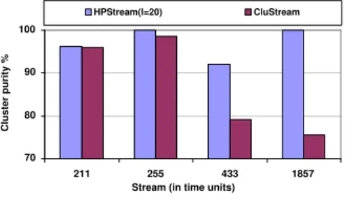
data sets. 70 80 90 100 211 255 433 1857
Stream (in time units)
C lu st er p ur ity % HPStream(l=20) CluStream
Figure 5: Quality comparison (Network Intrusion data set, horizon = 1, stream speed = 200)
70 80 90 100
1500 2500 3500 4500
Stream (in time units)
C lu st er p ur ity % HPStream(l=20) CluStream
Figure 6: Quality comparison (Network Intrusion data set, horizon = 10, stream speed = 100)
Figure 5 and Figure 6 show the clustering quality comparison results for the Network Intrusion Detec-tion data set. In the experiments CluStream used all
the 34 dimensions, while we set the average number of projected dimensions at 20 (i.e.,l= 20) forHPStream,
which means on average HPStreamused 20 projected
dimensions. In Figure 5, the stream speed is set at 200 points per time unit and horizonH = 1. We chose a se-ries of time points when there were some kind of attack connections happened. For example, at timeT = 211 there were 1 “phf” connection, 23 “portsweep” con-nections, and 176 “normal” connections during the past 1 horizon, while at time T = 1857, there were totally 79 “smurf”, 99 “teardrop”, and 22 “pod” at-tack connections for the last horizon. From Figure 5, we can see that HPStream has a very good
cluster-ing quality: its clustercluster-ing purity is always higher than 90% and better thanCluStream. For example, at time
T = 1857,HPStreamgrouped different attack
connec-tions into different clusters, while CluStream grouped
all kinds of attacks into one cluster, this is why
HP-Stream’s cluster purity is more than 20% higher than
that of CluStream. We also set the stream speed at
100 points per time unit and horizon H at 10 to test the clustering quality, Figure 6 shows the results. Ex-cept at time T = 2500, HPStreamalways has a much
higher cluster purity than CluStream. We checked the
original class labels for the connections in the last ten horizons from the current time 2500 and found all the connections belong to one attack type, “smurf”. As a result, no matter what clustering algorithms we used, they would always have a 100% cluster purity and this does not meanCluStreamcan do good job in this case.
70 75 80 85 90 95 100 160 320 640 1280 2560
Stream (in time units)
C lu st er p ur ity % HPStream(l=8) CluStream
Figure 7: Quality comparison (Forest CoverType data set, horizon=1, stream speed=200)
We also tested the clustering quality of HPStream
for another real data set, Forest CoverType. For this data set, we set the average number of projected di-mensions at 8 (i.e.,l= 8). Figure 7 and Figure 8 show the clustering quality comparison results. In Figure 7, we set the stream speed at 200 points per time unit and compute the cluster purity at different time for the last one horizon (i.e., H = 1). Figure 7 shows
that HPStream always has higher cluster purity than
CluStream, even for such a data set with a not very
high dimensionality (here d= 10). We then changed the stream speed to 100 points per time unit and hori-zon H to 10 and compare the cluster quality for the two algorithms. Figure 8 shows the similar picture:
HPStreamalways has higher cluster purity than
CluS-tream. 60 65 70 75 80 85 90 95 200 400 800 1600 3200
Stream (in time units)
C lu st er p ur ity % HPStream(l=8) CluStream
Figure 8: Quality comparison (Forest CoverType data set, horizon = 10, stream speed = 100)
60 70 80 90
100 200 300 400 500
Stream (in time units)
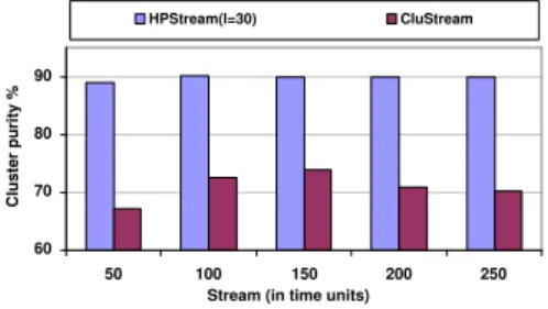
C lu st er p ur ity % HPStream(l=30) CluStream
Figure 9: Quality comparison (Synthetic data set B100kC10D50L30, horizon = 1, stream speed = 200)
60 70 80 90
50 100 150 200 250
Stream (in time units)
C lu st er p ur ity % HPStream(l=30) CluStream
Figure 10: Quality comparison (Synthetic data set B100kC10D50L30, horizon = 10, stream speed = 400)
B100kC10D50L30, to test the clustering quality.
This data set contains 100,000 points that has a total dimensionality of 50 and an average number of projected dimensions 30. The data points belong to 10 different clusters. In the experiments, we set
l at 30 for HPStream. As Figure 9 shows when we
set the stream speed at 200 points per time unit and horizon at 1, HPStream consistently has much
better clustering quality thanCluStream: On average,
the cluster purity of HPStream is about 20% higher
than that ofCluStream. We then changed the stream
speed to 400 points per time unit and used a lager horizon,H = 10, to test the clustering quality. Figure 10 shows that the cluster purity of the HPStream
algorithm is always over 15% higher than that of
CluStream.
Efficiency test. We used both theNetwork Intrusion
Detection and Forest CoverType data sets to test the
efficiency ofHPStreamagainstCluStream. Because the
CluStream algorithm needs to periodically store away
the current snapshot ofmicro-clustersunder the
Pyra-midal Time Framework, we implemented two versions
of theCluStreamalgorithm: One uses disk to maintain
the snapshots of micro-clusters, and the other stores the snapshots ofmicro-clusters in memory. The algo-rithm efficiency is measured by the stream processing rate versus progression of the stream, which is defined as the inverse of the time required to process the last 1000 points (The unit is in points/second). In the ex-periments, we fixed the stream speed at 200 points per second.
Figure 11 shows the stream processing rate for Network Intrusion data set, from which we can see
1000 10000
200 300 400 500 600 700 800 900 1000
Number of points processed per second
Stream (in time units) CluStream(memory)
HPStream CluStream(disk)
Figure 11: Stream Processing Rate (Network Intrusion data set, stream speed = 200)
10000 100000
200 300 400 500 600 700 800 900 1000
Number of points processed per second
Stream (in time units) CluStream(memory)
HPStream CluStream(disk)
Figure 12: Stream Processing Rate (Forest CoverType data set, stream speed = 200)
that HPStream is more efficient than the disk-based
CluStream algorithm and is only marginally slower
than the memory-based CluStream algorithm.
How-ever, as we know, the memory-based CluStream
al-gorithm will consume much more memory than HP-Stream. In addition, for this data set, the processing
rate of HPStream is very stable and is around 11,000
points/second, which means HPStreamcan support a
high stream speed at 10,000 points/second. Figure 12 shows the stream processing rate for theForest Cover-Type data set. Because this data set has a smaller di-mensionality than the Network Intrusion data set, all these algorithms have a higher stream processing rate. For example, both HPStream and the memory-based
CluStream algorithms have a stream processing speed
around 35,000 points/second. Similarly,HPStreamhas
a higher processing speed than the disk-based
CluS-treamalgorithm while consumes less memory than the
memory-basedCluStream algorithm.
4.2 Sensitivity Analysis
In sensitivity analysis, we show how sensitive the clus-tering quality is in relevance to the average projected dimensionality, the radius threshold, and the decay rate.
Choice of the average projected dimensional-ity l. The average projected dimensionality l plays an important role in choosing a proper set of pro-jected dimensions that are used by HPStream to do
clustering, we want to know how sensitive it is in af-fecting the clustering quality. Because we know the true average projected dimensionality in advance for synthetic data sets, we will use the synthetic data
setB100kC10D50L30 to test the clustering quality by
choosing different average projected dimensionalityl.
70 80 90 100
100 200 300 400 500 Stream (in time units)
C lu st er p ur ity % l=10 l=20 l=30 l=40 l=50
Figure 13: Choice of l (Synthetic data set B100kC10D50L30, horizon = 5, stream speed = 200)
70 80 90 100
50 100 150 200 250
Stream (in time units)
C lu st er p ur ity % l=10 l=20 l=30 l=40 l=50
Figure 14: Choice of l (Synthetic data set B100kC10D50L30, horizon = 10, stream speed = 400)
B100kC10D50L30 was generated with an average
projected dimensionality l = 30, in our experiments we used a series of different l’s, i.e., {10, 20, 30, 40, 50}, to test the clustering quality. We first fixed the stream speed at 200 points per time unit and horizon at 5. Figure 13 shows the result. As we can see, overall
l = 30 can lead to the best cluster purity, and a too small l at 10 or a too large l at 50 will generate very poor clustering quality. In addition, the cluster purity forl = 20 orl= 40 is very similar to that for l = 30, which suggests as long as we choose a value forlin the range from 20 to 40,HPStreamwill have a very good
clustering quality.
We then set the stream speed at 400 points per time unit and horizon H at 10, and did the same set of tests. Figure 14 shows the result, which is very similar to that in Figure 13. In addition, under the same settings and with the same data set, from Figure 10 we knowCluStreamnever generated a cluster purity
higher than 80%, as a result, no matter what value we choose for l from 20, 30, or 40, HPStreamalways has
much better cluster purity thanCluStream
The above experiments about the sensitivity of the average projected dimensionalityldemonstrate that as long as we choose for l a value not too deviated from the true average projected dimensionality, HPStream
will have a high clustering quality. We also did some further tests using the Network Intrusion Detection data set and foundHPStreamalways generated similar
clustering solution if we chose forla value in the range from 20 to 30.
Choice of the radius threshold. Although the average projected dimensionality l provides a very flexible and natural way for HPStream to pick the
set of well correlated dimensions for clustering high-dimensional data, however, in some cases a radius threshold may be more intuitively chosen as an al-ternative in selecting the set of projected dimen-sions. This quality-controlled parameter would allow the number of projected dimensions evolve over the stream. For example, among the 34 dimensions for Network Intrusion Detection data set, most of them have a deviation 0 for a certain type of connections. If the user has this knowledge in advance, he may choose a radius threshold which is very close to 0 in defining the set of projected dimensions.
70 80 90 100
211 255 433 1857
Stream (in time units)
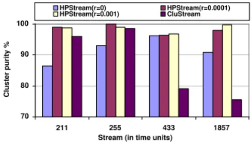
C lu st er p ur ity % HPStream(r=0) HPStream(r=0.0001) HPStream(r=0.001) CluStream
Figure 15: Quality comparison based on the radius threshold (Network Intrusion data set, horizon = 1, stream speed = 200)
Figure 15 shows the test result for the Network In-trusion data set by setting the stream speed at 200 points per time unit and horizon H at 1. In the ex-periments, we test against CluStream the clustering
quality ofHPStreamwith varying radius threshold as
an input parameter. The result shows that if we set the radius threshold at 0.001 or 0.0001,HPStream
al-ways has much better clustering quality than CluS-tream. For example, at timeT = 1857, the cluster
pu-rity of HPStream is more than 20% higher than that
of CluStream. This suggests a radius threshold in the
range [0.0001,0.001] could make HPStream generate
very good clustering solutions for the Network Intru-sion data set.
Choice of the decay rate λ. Another important parameter for HPStream is the decay rate λ, which
defines the importance of the historical data. In sec-tion 4.1, we setλat a moderate value, 0.5, with which
HPStreamshowed much better clustering quality than
CluStream. We also did several experiments to
iso-late the effect of decay rate λ by changing λ from a small value to a large one. We used the synthetic data
setB100kC10D50L30 and set the stream speed at 200
points per time unit and average projected dimension-ality l= 30 to test the cluster purity of HPStreamat
60 70 80 90 100 110 0.001 0.01 0.1 1 Cluster purity % Decay rate HPStream CluStream
Figure 16: Choice of decay rateλ(Synthetic data set B100kC10D50L30, stream speed = 200, H = 10, time units = 100, l= 30)
time T = 100 with horizon 10. Figure 16 shows the results corresponding to a series of decay rates, 0.0005, 0.005, 0.05, 0.5, 1, 2, and 4. If 0.0005≤ λ≤2, HP-Stream has a relatively stable cluster purity which is
much better than that of CluStream. However, when
we use a very high value forλlike 4,HPStream’s
qual-ity deteriorates quickly, but still is a little better than that of CluStream. We note that the choice of λ= 4
represents a pathological case in which the clusters are determined based on only a small number of recently arriving data points. In such cases, both algorithms tends to show relatively similar behavior.
4.3 Scalability Test
The scalability tests presented below show that
HP-Stream is linearly scalable with both dimensionality
and the number of clusters. We have already shown
thatHPStreamhas very stable stream processing speed
along with the progression of the stream for the two real data sets. High scalability in terms of dimension-ality and the number of clusters is also very critical to the success of a high-dimensional clustering algorithm. We generated a series of synthetic data sets to test the scalability ofHPStream. 0 20 40 60 80 100 120 140 10 20 30 40 50 60 70 80 runtime in seconds Number of dimensions B400kC20 B200kC10 B100kC5
Figure 17: Scalability with dimensionality (stream speed = 100,l= 0.8×d)
We first generated 3 data sets with varying num-ber of dimensions to test the scalability against
di-mensionality. B100kC5 contains 100K points and 5 natural clusters, B200kC10 contains 200K points and 10 clusters, and B400kC20 contains 400K points and 20 clusters. For each series of data sets, we generated 4 data sets with dimensionality d set at 10, 20, 40, and 80, respectively. The average number of projected dimensions for each data set is set at 0.8×dand the stream speed is set at 100 points per time unit. Figure 17 shows that when we varied the dimensionality from 10 to 80,HPStreamhas linear increase in runtime for
data sets with different number of points and different number of clusters. For example, for data set series B200kC10, the runtime increases from 6.579 seconds to 49.401 seconds when the dimensionality is changed from 10 to 80. 0 10 20 30 40 50 60 70 80 90 5 10 15 20 25 30 35 40 runtime in seconds Number of clusters B400kD40 B200kD20 B100kD10
Figure 18: Scalability with number of clusters (stream speed=100,l= 0.6×d)
To test the scalability against the number of nat-ural clusters, we generated another 3 series of data sets with varying number of clusters. B100kD10 con-tains 100K 10-dimensional data points, B200kD20 has 200K 20-d data points, and B400kD40 has 400K 40-d data points. For each series of data sets, we generated 4 data sets with the number of natural clusters set at 5, 10, 20, and 40, respectively. The average num-ber of projected dimensions for each data set is set at 0.6×d and the stream speed at 100 points per time unit. Figure 18 shows that the runtime of HPStream
has very good scalability in terms of the number of clusters for data sets with different number of points and dimensionality. The high scalability ofHPStream
in terms of the number of clusters stems from both the algorithm design and implementation. Among the three most costly functions inHPStreamalgorithm, the
computation ofFindLimitingRadiushas nothing to do with the number of clusters, FindProjectedDist is lin-early scalable to the the number of clusters, whereas
forComputeDimensions, we can exploit the temporal
locality to improve its efficiency: At a certain period, the points usually only belong to a small number of clusters, and only the dimensions of these clusters will be changed during the past period with the necessity to re-compute their radii.
5
Discussion
Our experiments have shown that the HPStream
framework leads to accurate and efficient high-dimensional stream clustering. This framework can be extended in many ways to assist stream data mining.
First, some methodologies, such as the cluster struc-ture and micro-clustering ideas, though designed for projected stream clustering, can be applied to pro-jected clustering of non-stream data as well. Moreover, the method worked out here for high-dimensional pro-jected stream clustering represents a general method-ology, independent of particular evaluation measures and implementation techniques. For example, one can change the distance measure from Euclidean distance to other measures, or change detailed clustering algo-rithm, such ask-means, to other methods, the general methodology should still be applicable. However, it is interesting to work out the detail implementation techniques for particular applications.
Second, one extension of the framework is to use tilted time windows to store data at different time granularity. This may take somewhat more space in cluster structure, however, it may give user more flex-ibility to dynamically assign or modify fading ratio, as well as to discover clusters at more flexibly specified windows or time periods to facilitate the discovery of cluster evolution regularity.
Finally, this study may promote the development of new streaming data mining functions, such as stream classification and similarity analysis based on dynam-ically discovered projected clusters.
6
Conclusions
We have presented a new framework, HPStream, for
high-dimensional projected clustering of data streams. It finds projected clusters in particular subsets of the dimensions by maintaining condensed representations of the clusters over time. The algorithm provides bet-ter quality clusbet-ters than full dimensional data stream clustering algorithms. We tested the algorithm on a number of real and synthetic data sets. In each case, we found that the HPStreamalgorithm was more
ef-fective than the full dimensionalCluStreamalgorithm.
High-dimensional projected clustering of data streams opens a new direction for exploration of stream data mining. With this methodology, one can treat projected clustering as a preprocessing step, which may promote more effective methods for stream classification, similarity, evolution and outlier analysis.
References
[1] C. C. Aggarwal. A Human-Computer Interactive Method for Projected Clustering. IEEE
Transac-tions on Knowledge and Data Engineering, 16(4),
448–460, 2004.
[2] C. C. Aggarwal, C. Procopiuc, J. Wolf, P. S. Yu, J.-S. Park. Fast algorithms for projected clustering.
ACM SIGMOD Conference, 1999.
[3] C. C. Aggarwal, J. Han, J. Wang, P. Yu. A Frame-work for Clustering Evolving Data Streams.VLDB
Conference, 2003.
[4] C. C. Aggarwal. An Intuitive Framework for Un-derstanding Changes in Evolving Data Streams.
ICDE Conference, 2002.
[5] C. C. Aggarwal. A Framework for Diagnosing Changes in Evolving Data Streams. ACM
SIG-MOD Conference, pp. 575–586, 2003.
[6] R. Agrawal, J. Gehrke, D. Gunopulos, P. Ragha-van. Automatic Subspace Clustering of High Di-mensional Data for Data Mining Applications.
ACM SIGMOD Conference,1998.
[7] M. Ankerst, M. Breunig, H.-P. Kriegel, J. Sander. OPTICS: Ordering Points To Identify the Cluster-ing Structure. ACM SIGMOD Conference, 1999. [8] B. Babcock, S. Babu, M. Datar, R. Motwani, J.
Widom. Models and Issues in Data Stream Sys-tems,ACM PODS Conference, 2002.
[9] C. Cortes, K. Fisher, D. Pregibon, A. Rogers, F. Smith. Hancock: A Language for Extracting Sig-natures from Data Streams. ACM SIGKDD Con-ference, 2000.
[10] P. Domingos, G. Hulten. Mining High-Speed Data Streams.ACM SIGKDD Conference, 2000. [11] F. Farnstrom, J. Lewis, C. Elkan. Scalability for
Clustering Algorithms Revisited.SIGKDD
Explo-rations, 2(1):51-57, 2000.
[12] J. Feigenbaum et al. Testing and spot-checking of data streams.ACM SODA Conference, 2000. [13] S. Guha, N. Mishra, R. Motwani, L. O’Callaghan.
Clustering Data Streams.IEEE FOCS Conference, 2000.
[14] S. Guha, R. Rastogi, K. Shim. CURE: An Effi-cient Clustering Algorithm for Large Databases.
ACM SIGMOD Conference, 1998.
[15] A. Jain, R. Dubes. Algorithms for Clustering Data, Prentice Hall,New Jersey, 1998.
[16] R. Ng, J. Han. Efficient and Effective Clustering Methods for Spatial Data Mining.Very Large Data
Bases Conference, 1994.
[17] L. O’Callaghan, N. Mishra, A. Meyerson, S. Guha, R. Motwani. Streaming-Data Algorithms For High-Quality Clustering. ICDE Conference, 2002.
[18] T. Zhang, R. Ramakrishnan, M. Livny. BIRCH: An Efficient Data Clustering Method for Very Large Databases. ACM SIGMOD Conference,