Contents lists available atScienceDirect
Journal of Multivariate Analysis
journal homepage:www.elsevier.com/locate/jmva
Nonparametric rank-based tests of bivariate extreme-value dependence
Ivan Kojadinovic
a,∗,1, Jun Yan
baLaboratoire de Mathématiques et Applications, UMR CNRS 5142, Université de Pau et des Pays de l’Adour, B.P. 1155, 64013 Pau Cedex, France bDepartment of Statistics, University of Connecticut, 215 Glenbrook Road, U-4120, Storrs, CT 06269, USA
a r t i c l e i n f o
Article history:
Received 16 February 2010 Available online 1 June 2010 AMS subject classifications: 62H15
62G32 Keywords: Contiguity
Extreme-value copulas Local power comparisons Multiplier central limit theorem Pseudo-observations
Ranks
a b s t r a c t
A new class of tests of extreme-value dependence for bivariate copulas is proposed. It is based on the process comparing the empirical copula with a natural nonparametric rank-based estimator of the unknown copula under extreme-value dependence. A multiplier technique is used to compute approximatep-values for several candidate test statistics. Extensive Monte Carlo experiments were carried out to compare the resulting procedures with the tests of extreme-value dependence recently studied in Ben Ghorbal et al. (2009) [1] and Kojadinovic and Yan (2010) [19]. The finite-sample performance study of the tests is complemented by local power calculations.
©2010 Elsevier Inc. All rights reserved.
1. Introduction
Extreme-value copulas appear in extreme-value theory as the limits of copulas of componentwise maxima in random samples [8,15,16]. This makes them natural tools for modeling the dependence between extreme observations in fields such as finance [23], insurance [7] or hydrology [27]. Their use, however, is not restricted to the statistical modeling of extremes as such copulas may prove to be appropriate dependence models for any data set exhibiting positive dependence.
Any extreme-value copula can be represented in terms of itsPickands dependence function[25,5,17,16]. For a bivariate copulaC, this representation becomes a characterization and takes the form
C
(
u, v)
=
exp log(
uv)
A log(v)
log(
uv)
,
u, v
∈
(
0,
1),
(1)whereA
: [
0,
1] → [
1/
2,
1]
, the Pickands dependence function, is convex and satisfies max(
t,
1−
t)
≤
A(
t)
≤
1 for all t∈ [
0,
1]
.Let
(
X1,
Y1), . . . , (
Xn,
Yn)
be a random sample from an unknown bivariate cumulative distribution function (c.d.f.)Hwithunknown continuous marginsFandG, and unknown copulaC. In order to reduce the number of candidate copula families that could be used as models forC, one natural step is to test whetherC belongs to the class of extreme-value copulas. Ghoudi, Khoudraji and Rivest were the first to propose a test of bivariate extreme-value dependence [15]. Their test, based on the bivariate probability integral transformation, was thoroughly revisited in [1]. A second test, based on the character-ization of extreme-value copulas as max-stable copulas, was recently proposed in [19].
The aim of this work is to derive a third class of tests of extreme-value dependence for bivariate copulas, and to compare its finite-sample performance and local limiting power with those of its two competitors mentioned above.
∗Corresponding author.
E-mail addresses:[email protected](I. Kojadinovic),[email protected](J. Yan). 1 Formerly with the Department of Statistics of the University of Auckland, New Zealand. 0047-259X/$ – see front matter©2010 Elsevier Inc. All rights reserved.
The proposed class of tests is based on the process comparing the empirical copula with another natural nonparametric estimator of the unknown copula derived under the hypothesis of extreme-value dependence. The latter estimator is constructed from a rank-based version of the Capéraà–Fougères–Genest estimator [3] of the Pickands dependence function recently studied in [14]. As the empirical process on which the proposed class of tests is based has an unwieldy limiting distribution, a multiplier approach inspired by that suggested in [26] is used to compute approximatep-values for several candidate test statistics.
The paper is organized as follows. Section2is devoted to an in-depth description of the proposed tests: the empirical process on which the tests are based is thoroughly studied and the computation of asymptotically valid approximatep -values for the test statistics is explained in detail. Section3partially reports the results of a large scale Monte Carlo study comparing the finite-sample performance of various versions of the tests with those of the tests of extreme-value depen-dence proposed in [1,19]. These experiments are complemented by asymptotic local power calculations in Section4. The last section contains methodological recommendations and concluding remarks. All the proofs are relegated to theAppendices. The following notational conventions are used in the paper. For anyx
,
y∈
R, min(
x,
y)
and max(
x,
y)
are denoted by x∧
yandx∨
y, respectively. Furthermore,`
∞(
S)
represents the space of bounded real-valued functions on the setS, whileC
(
[
a,
b]
)
represents the space of continuous real-valued functions on the real closed interval[
a,
b]
; both are equipped with the uniform metric. The arrow;denotes weak convergence while the set of bivariate extreme-value copulas, i.e., copulas characterized by(1), is denoted byE V.Note finally that all the tests studied in this work are implemented in the R package
copula
[20] available on the Comprehensive R Archive Network.2. Description of the test
The empirical process at the root of the proposed new class of tests of extreme-value dependence involves the comparison of the empirical copula with a natural nonparametric estimator of the unknown copula derived under the hypothesisH0
:
C
∈
E V. The latter estimator is obtained by replacing the unknown Pickands dependence function in characterization(1)by a consistent rank-based estimator of it recently studied in [14].
2.1. Nonparametric estimation of C
A natural nonparametric estimator of the underlying copulaC
(
u, v)
=
H{
F−1(
u),
G−1(v)
}
is the empirical copula [4]. It is usually defined as Cn(
u, v)
=
1 n nX
i=1 1(
Ui,n≤
u,
Vi,n≤
v),
u, v
∈ [
0,
1]
,
where
(
U1,n,
V1,n), . . . , (
Un,n,
Vn,n)
arepseudo-observationsfromCcomputed from the data by(
Ui,n,
Vi,n)
=
(
Fn(
Xi),
Gn(
Yi))
for alli∈ {
1, . . . ,
n}
withFnandGnbeing the rescaled empirical counterparts ofFandGrespectively defined byFn
(
x)
=
1 n+
1 nX
i=1 1(
Xi≤
x)
and Gn(
y)
=
1 n+
1 nX
i=1 1(
Yi≤
y),
x,
y∈
R.
Under the assumption thatChas continuous partial derivatives on
(
0,
1)
2, it is well known [9,6,31] that the weak limit of the empirical copula process√
n(
Cn−
C)
isC
(
u, v)
=
α(
u, v)
−
C[1](
u, v)α(
u,
1)
−
C[2](
u, v)α(
1, v),
u, v
∈ [
0,
1]
,
(2)whereC[j]denotes the partial derivative ofCwith respect to thejth argument and
α
is aC-Brownian bridge, i.e., a tight centered Gaussian process on[
0,
1]
2with covariance functionE[
α(
u, v)α(
u0, v
0)
] =
C(
u∧
u0, v
∧
v
0)
−
C(
u, v)
C(
u0, v
0)
,u
, v,
u0, v
0∈ [
0,
1]
.2.2. Nonparametric estimation of A
Genest and Segers [14] have recently studied two rank-based estimators of the Pickands dependence functionAappearing in representation(1). These two estimators are the rank-based versions of the two best-known nonparametric estimators ofA, namely the Pickands estimator [25] and the Capéraà–Fougères–Genest estimator [3]. The latter estimator was found to behave better in finite samples in several studies [14,12]. The results of the Monte Carlo experiments carried out in this work and partially reported in Section3concur with this conclusion. For this reason, we present the derivation of the proposed tests only when based on the Capéraà–Fougères–Genest estimator. The analogue expressions based on the Pickands estimator can be recoveredmutatis mutandis.
Assume thatC is an extreme-value copula and, as in the previous subsection, let
(
U1,n,
V1,n), . . . , (
Un,n,
Vn,n)
be the pseudo-observations fromCcomputed from the original data. Furthermore, letfor everyi
∈ {
1, . . . ,
n}
, and letξ
i,n(
0)
=
Si,n,
ξ
i,n(
1)
=
Ti,n,
andξ
i,n(
t)
=
Si,n 1−
t∧
Ti,n t,
for everyi
∈ {
1, . . . ,
n}
and anyt∈
(
0,
1)
. The rank-based version of the Capéraà–Fougères–Genest estimator is then defined by An(
t)
=
exp(
−
γ
−
1 n nX
i=1 logξ
i,n(
t)
)
,
t∈ [
0,
1]
,
whereγ
= −
R
∞ 0 log(
x)
e−xdx
≈
0.
577 is Euler’s constant. The previous estimator can be expressed in terms of the empirical copula as An(
t)
=
exp−
γ
+
Z
1 0 Cn(
x1−t,
xt)
−
1(
x>
e−1)
dx xlogx,
t∈ [
0,
1]
.
The limiting behavior ofAnfollows from [14, Theorem 3.2]. Provided that the true Pickands dependence functionAis twice continuously differentiable on
(
0,
1)
(which we will assume in the rest of the paper), we have that√
n{
An(
t)
−
A(
t)
}
;A(
t)
=
A(
t)
Z
1 0 C(
x1−t,
xt)
dx xlogx,
(3) inC(
[
0,
1]
)
, whereCis defined in(2).To ensure that the endpoint constraintsAn
(
0)
=
An(
1)
=
1 are satisfied, the previous estimator can be corrected as suggested in [3]. This yields the corrected versionAn,c
(
t)
=
exp{
logAn(
t)
−
(
1−
t)
logAn(
0)
−
tlogAn(
1)
}
,
t∈ [
0,
1]
,
which generally behaves better in small samples than the uncorrected one. For this reason, in the rest of the paper, we shall always work with the above corrected version. Note however thatAnandAn,cbecome indistinguishable asntends to infinity [14, Section 2.4].
2.3. Test process and test statistics
In view of the previous subsection and of representation(1), it seems sensible to define a nonparametric estimator of the unknown copula under extreme-value dependence as
CAn,c
(
u, v)
=
exp log(
uv)
An,c log(v)
log(
uv)
,
u, v
∈
(
0,
1).
A natural way of testing extreme-value dependence then consists of comparing the empirical copula Cn, which is a nonparametric estimator ofC whetherH0
:
C∈
E Vis true or not, withCAn,c. More formally, this amounts to basing tests of extreme-value dependence on the empirical processDn
=
√
n(
Cn−
CAn,c),
i.e., Dn(
u, v)
=
√
n Cn(
u, v)
−
exp log(
uv)
An,c log(v)
log(
uv)
,
u, v
∈
(
0,
1).
(4)The following result, proved inAppendix A, describes the asymptotic behavior of the test process(4)underH0.
Proposition 1. Let a
,
b∈
(
0,
1)
, a<
b, and suppose that A is twice continuously differentiable on(
0,
1)
. Then, underH0, Dn;Din`
∞(
[
a,
b]
2)
, where D(
u, v)
=
C(
u, v)
−
exp log(
uv)
A log(v)
log(
uv)
log(
uv)
A log(v)
log(
uv)
.
(5)The realsaandbin the previous proposition can be chosen arbitrarily close to 0 and 1, respectively. We will explain in Section3how they were chosen in practice.
As candidate test statistics, we restricted our attention to the two Cramér–von Mises functionals Sn
=
Z
[a,b]2Dn(
u, v)
2dudv
and Tn=
Z
[a,b]2Dn(
u, v)
2dCn(
u, v).
Kolmogorov–Smirnov statistics were not considered because, from our experience, Cramér–von Mises statistics generally lead to more powerful tests.
2.4. Multiplier central limit theorems
The use of the weak limit of the test processDnestablished inProposition 1to compute asymptoticp-values for the statisticsSnandTnappears unwieldy. We therefore resort to a multiplier approach to obtain approximatep-value forSnand Tnin the spirit of that used in [26,21]. The idea is to use multipliers to generate a large number of approximate independent realizations of the weak limitDof the test process, derive the corresponding approximate independent realizations ofSn andTn, and finally compute approximatep-values using the resulting empirical c.d.f.s.
Before stating the key result that provides an asymptotic justification to the adopted approach, let us first introduce additional notation. LetNbe a large integer and letZi(k),i
=
1, . . . ,
n,k=
1, . . . ,
N, be i.i.d. random variables with mean 0 and variance 1 independent of the data(
X1,
Y1), . . . , (
Xn,
Yn)
. For anyk∈ {
1, . . . ,
N}
, letα
(k) n(
u, v)
=
1√
n nX
i=1 Zi(k)1(
Ui,n≤
u,
Vi,n≤
v)
−
Cn(
u, v)
=
√
1 n nX
i=1(
Zi(k)− ¯
Z(k))
1(
Ui,n≤
u,
Vi,n≤
v),
u, v
∈ [
0,
1]
,
(6) whereZ¯
(k)=
n−1P
n i=1Z (k) i .In order to obtain approximate independent copies of the processDdefined in(5), it is necessary to estimate the unknown partial derivatives ofCthat appear in the expression ofC, and therefore in that ofA; see(2)and(3), respectively. A first way to proceed consists of using the generic estimators proposed in [26, page 380] (see also [19, Proposition 2]). For
(
u, v)
∈
(
0,
1)
2, these are respectively defined byCn[1]
(
u, v)
=
Cn(
u+
n −1/2, v)
−
C n(
u−
n−1/2, v)
2n−1/2,
and Cn[2](
u, v)
=
Cn(
u, v
+
n −1/2)
−
C n(
u, v
−
n−1/2)
2n−1/2.
Under extreme-value dependence, starting from characterization(1), alternative natural nonparametric estimators were proposed in [21]. For any
(
u, v)
∈
(
0,
1)
2, lettuv
=
log(v)/
log(
uv)
. The partial derivativesC[1]andC[2]can then beesti-mated, for
(
u, v)
∈
(
0,
1)
2, by CA[1n],c(
u, v)
= { ˆ
An,c(
tuv)
−
tuvA0n,c(
tuv)
}
(
uv)
An,c(tuv)−(1−tuv),
and CA[2] n,c(
u, v)
= { ˆ
An,c(
tuv)
+
(
1−
tuv)
A 0 n,c(
tuv)
}
(
uv)
An,c(tuv)−tuv,
whereAˆ
n,c=
(
An,c∧
1)
∨
I∨
(
1−
I)
,Iis the identity function, andA0n,c
(
t)
=
An,c{
(
t+
n−1/2
)
∧
1} −
An,c
{
(
t−
n−1/2)
∨
0}
2n−1/2
,
t∈
(
0,
1).
Now, for anyk
∈ {
1, . . . ,
N}
and(
u, v)
∈
(
0,
1)
2, let C(nk)(
u, v)
=
α
( k) n(
u, v)
−
C [1] n(
u, v)α
( k) n(
u,
1)
−
C [2] n(
u, v)α
( k) n(
1, v),
(7) let C(Akn),c(
u, v)
=
α
(k) n(
u, v)
−
C [1] An,c(
u, v)α
(k) n(
u,
1)
−
C [2] An,c(
u, v)α
(k) n(
1, v),
(8) let A(nk)(
t)
=
An,c(
t)
Z
1 0 C(Akn),c(
x 1−t,
xt)
dx xlogx,
(9) and let D(nk)(
u, v)
=
C( k) n(
u, v)
−
exp log(
uv)
An,c log(v)
log(
uv)
log(
uv)
A(nk) log(v)
log(
uv)
.
(10)Proposition 2. Let a
,
b∈
(
0,
1)
, a<
b, and suppose that A is twice continuously differentiable on(
0,
1)
. Then, underH0, Dn,
D(n1), . . . ,
D(nN); D
,
D(1), . . . ,
D(N)in
`
∞(
[
a,
b]
2)
⊗(N+1), whereD(1), . . . ,
D(N)are independent copies of the processDdefined in(5).As shall be discussed in Section2.6, alternative definitions of the processD(nk)can be considered depending on whether Cn(k)orC(Akn),c are used in(9)and(10). The definitions adopted above led to the tests with the best finite-sample behavior. More details will be given in Section3.
Next, for anyk
∈ {
1, . . . ,
N}
, let Sn(k)=
Z
[a,b]2D
(k)
n
(
u, v)
2dudv.
From the previous proposition and the continuous mapping theorem, we immediately have that, underH0,
Sn
,
Sn(1), . . . ,
S(nN); S
,
S(1), . . . ,
S(N) in[
0,
∞
)
⊗(N+1), whereSis the weak limit ofSn, andS(1)
, . . . ,
S(N)are independent copies ofS. This suggests computing an approximatep-value forSnas1 N N
X
k=1 1 Sn(k)≥
Sn.
Similarly, for anyk
∈ {
1, . . . ,
N}
, let Tn(k)=
Z
[a,b]2D (k) n(
u, v)
2dC n(
u, v).
An approximatep-value forTnis then computed byN−1
P
N k=11 Tn(k)≥
Tn .In order to carry out the tests, it is necessary to compute the integral appearing in the expression ofA(nk)given in(9). As shown in [21], for anyk
∈ {
1, . . . ,
N}
and anyt∈
(
0,
1)
, we haveZ
1 0 C(Akn),c(
x 1−t,
xt)
dx xlogx= −
1√
n nX
i=1(
Zi(k)− ¯
Z(k))
log Si,n 1−
t∧
Ti,n t−
√
1 n{ ˆ
An,c(
t)
−
tA 0 n,c(
t)
}
nX
i=1 Zi(k)Z
1 0 xAˆn,c(t)−(1−t) 1(
Ui,n≤
x1−t)
−
b
x 1−t(
n+
1)
c
n dx xlogx−
√
1 n{ ˆ
An,c(
t)
+
(
1−
t)
A 0 n,c(
t)
}
nX
i=1 Zi(k)Z
1 0 xAˆn,c(t)−t 1(
Vi,n≤
xt)
−
b
xt(
n+
1)
c
n dx xlogx,
where, for anyy
≥
0,b
yc
denotes the integer part ofy. Note that the two integrals appearing in the right-hand side of the previous expression are not indefinite as the integrands are zero whenxgets close to 0 or 1. They are computed numerically in our implementation.2.5. Consistency of the tests
The work of Garralda-Guillem [10] implies that extreme-value copulas are left-tail decreasing (LTD) in both arguments; see e.g. [24, Section 5.2.2]. These dependence conditions are actually satisfied by the most popular bivariate copulas with positive dependence such as the Clayton, Frank, normal,t and Plackett. IfChas a continuous density and is LTD in both arguments but is not necessarily an extreme-value copula, it was shown in [12, Proposition 2] that
√
n(
An,c−
AC)
;ACinC
(
[
0,
1]
)
, where AC(
t)
=
exp−
γ
+
Z
1 0 C(
x1−t,
xt)
−
1(
x>
e−1)
dx xlogx,
t∈ [
0,
1]
,
(11) and AC(
t)
=
AC(
t)
Z
1 0 C(
x1−t,
xt)
dx xlogx,
t∈ [
0,
1]
.
The functionACactually turns out to be well defined for any copulaCand reduces to the Pickands dependence functionA whenCis an extreme-value copula.
To study the consistency of the proposed tests, assume thatChas a continuous density and is LTD in both arguments without being an extreme-value copula. Also, let
CAC
(
u, v)
=
exp log(
uv)
AC log(v)
log(
uv)
,
u, v
∈
(
0,
1).
Then, the test processDncan be decomposed as√
n(
Cn−
CAn,c)
=
√
n(
Cn−
C)
−
√
n(
CAn,c−
CAC)
+
√
n(
C−
CAC).
Proceeding as in the proof ofProposition 1, it can be verified that√
n(
Cn−
C)
−
√
n(
CAn,c−
CAC)
converges weakly to C(
u, v)
−
exp log(
uv)
AC log(v)
log(
uv)
log(
uv)
AC log(v)
log(
uv)
in`
∞(
[
a,
b]
2)
. IfC6=
C AC, then sup(u,v)∈(0,1)2√
n
|
C(
u, v)
−
CAC(
u, v)
|
tends to infinity, which implies that any sensible statistic derived from the process√
n(
Cn−
CAn,c)
will tend to infinity.Interestingly enough, conclusions about the consistency of the studied tests can then be drawn when the functionACis convex, as stated in the following result proved inAppendix C.
Proposition 3. Assume that C has a continuous density and is LTD in both arguments without being an extreme-value copula. If the function ACis convex, then C
6=
CAC.As can be seen from [12, Figure 3], the functionACappears convex for the most frequently used bivariate copulas with positive dependence such as the Clayton, Frank, normal and Plackett. This suggests that the proposed class of tests will be consistent under a wide range of alternatives. An analytical proof of the convexity ofACfor non-extreme-value copulas that have a continuous density and that are LTD in both arguments is however still missing.
2.6. Alternative versions of the tests
Alternative versions of the tests can be obtained by replacingC(Akn),c byC(nk), or vice versa, in (9)and(10), respectively. Among the four possible definitions forD(nk), only two led to tests that were not too liberal for small sample size. The best rejection rates were obtained using the definition adopted in Section2.4. Slightly less powerful but faster tests were obtained by definingA(nk)as A(nk)
(
t)
=
An,c(
t)
Z
1 0 C(nk)(
x 1−t,
xt)
dx xlogx (12)instead of(9). Although all four possible versions are expected to be asymptotically equivalent, we were not able to prove an analogue ofProposition 2in this last case.
Unlike the version of the test described in Section2.4, the version based on the above definition ofA(nk)does not require the use of numerical integration to compute the integral appearing in its expression, and is therefore substantially faster. To see this, let
S+i,n
= −
log(
Ui,n+
n−1/2)
∧
n n+
1,
Si−,n= −
log(
Ui,n−
n−1/2)
∨
1 n+
1,
and Ti+,n= −
log(
Vi,n+
n−1/2)
∧
n n+
1,
Ti−,n= −
log(
Vi,n−
n−1/2)
∨
1 n+
1,
for everyi∈ {
1, . . . ,
n}
. Then, as shown in [21], for anyk∈ {
1, . . . ,
N}
and anyt∈
(
0,
1)
,Z
1 0 C(nk)(
x 1−t,
xt)
dx xlogx=
1√
n nX
i=1(
Zi(k)− ¯
Z(k))
"
−
log Si,n 1−
t∧
Ti,n t−
1 2√
n nX
j=1(
−
log S − j,n 1−
t∧
Tj,n t∧
Si,n 1−
t!
+
log S + j,n 1−
t∧
Tj,n t∧
Si,n 1−
t!
−
log Sj,n 1−
t∧
Tj−,n t∧
Ti,n t!
+
log Sj,n 1−
t∧
Tj+,n t∧
Ti,n t!)#
.
3. Finite-sample performance
The finite-sample performance of the tests described in the previous section was investigated in a large scale Monte Carlo experiment. As explained in Section2.6, four versions of the test based onSnand four versions of the test based onTnwere considered. The realsaandbappearing in the expressions of the statisticsSnandSn(k)were set to 1
/
mand 1−
1/
m, with m=
30. The resulting integrals were computed numerically using a grid ofm2uniformly spaced points on[
1/
m,
1−
1/
m]
2. Larger values ofmwere considered but this did not seem to improve the results. The statisticsTnandTn(k)were computed by settingaandbto 0 and 1, respectively, that is, asTn
=
1 n nX
i=1 Dn(
Ui,n,
Vi,n)
2 and Tn(k)=
1 n nX
i=1 D(nk)(
Ui,n,
Vi,n)
2,
respectively.The rejection rates of the eight tests mentioned above were compared with those of the test of extreme-value dependence described in [1] based on a variance estimator denoted
σ
ˆ
2n, and with those of the test proposed in [19] based on a statistic denotedT3,4,5,n.
To investigate the level of the tests, only the Gumbel–Hougaard (GH) copula and an asymmetric version of it were used. Indeed, one of the most surprising findings of the recent study of bivariate extreme-value copulas carried out in [12] is that the most frequently used such copulas,viz.the Gumbel–Hougaard, Galambos, Hüsler–Reiss and Student extreme-value, show striking similarities for a given degree of dependence. It therefore does not seem necessary to work with different extreme-value families. More variety in this class is obtained by using asymmetric extreme-value copulas constructed using Khoudraji’s device [18,11,22]. The asymmetric version of the Gumbel–Hougaard copula used in our study is denoted by aGH and is defined by
aGHθ,λ,κ
(
u, v)
=
u1−λv
1−κGHθ(
uλ, v
κ),
u, v
∈ [
0,
1]
, λ, κ
∈
(
0,
1]
, λ
6=
κ,
where GHθ is the c.d.f. of the Gumbel–Hougaard copula with parameter
θ
. Note that aGHθ,λ,κ is nothing else but the asymmetric logistic model introduced in [29,30]. In the experiments,θ
was set to 4, whileλ
andκ
were set to 0.4 and 0.95, respectively, so that data generated from this copula display strong asymmetries. For the Gumbel–Hougaard (GH) copula, three values ofθ
were considered, corresponding respectively to a Kendall’sτ
of 0.25, 0.5 and 0.75.To study the power of the tests, five non-extreme-value copulas were used: the Clayton (Cl), Frank (F), normal (N),t with 4 degrees of freedom (t-4) and Plackett (P). As previously, three levels of dependence, i.e.,
τ
∈ {
0.
25,
0.
5,
0.
75}
, were considered.Sample of sizesn
=
100, 200, 400 and 800 were generated. All the tests were carried out at the 5% significance level and empirical rejection rates were computed from 1000 random samples per scenario.A first finding of our extensive Monte Carlo study is that, among the four possible ways of defining the processesD(nk), only those described in Sections2.4and2.6gave tests that were not too liberal forn
=
100 and 200.A second rather accidental finding is that the use ofC
ˆ
ndefined byˆ
Cn(
u, v)
=
1 n+
1(
nX
i=1 1(
Ui,n≤
u,
Vi,n≤
v)
+
1 2)
,
u, v
∈ [
0,
1]
,
instead of Cn in the expressions of the statistics Sn and Tn (the expressions of Sn(k) and Tn(k) remaining unchanged) gave consistently less conservative and more powerful tests. Clearly, C
ˆ
n and Cn are asymptotically equivalent since sup(u,v)∈[0,1]2| ˆ
Cn(
u, v)
−
Cn(
u, v)
| ≤
1/
n. The results to be presented in the forthcoming tables are therefore those obtained whenCnis replaced byCˆ
nin the expressions ofSnandTn, i.e., in the expression ofDngiven in(4). The statistics resulting from this asymptotically negligible modification will be denoted bySˆ
nandTˆ
n, respectively.A third finding is that the tests based on the statisticsT
ˆ
nandTnwere more powerful than those based onSˆ
nandSnin all the scenarios under consideration.The rejection rates of the two best versions of the test based onT
ˆ
nare given inTables 1–3. They differ according to whether approximatep-values were computed using the alternative expressions given in Section2.6or those of Section2.4. We will refer to these two versions asTˆ
Cn andT
ˆ
nA, respectively. As can be seen fromTable 1, the testTˆ
Cn appears to be too conservative for small sample size. Its empirical levels seem to improve overall asnincreases, though the improvement seems to be slow when
τ
=
0.
75. The empirical levels ofTˆ
An, although not perfect, are globally more satisfactory for small sample size.
In terms of power, the testT
ˆ
An outperforms that based onT
ˆ
nC. As can be seen fromTable 2andTable 3, the difference between their rejection rates is substantial forn=
100 but decreases rather rapidly asnincreases. Forn=
800, the two tests are virtually equivalent as could have been expected.When compared to the tests based onT3,4,5,nand
σ
ˆ
n2, the testTˆ
nAis the most powerful when the data arise from the Frank or the Plackett copula andτ
∈ {
0.
5,
0.
75}
. Forτ
=
0.
25, it is outperformed by the test based onT3,4,5,n. For data setsTable 1
Rejection rate (in %) of the null hypothesis as observed in 1000 random samples of sizen=100, 200, 400 and 800 from the Gumbel–Hougaard copula (GH) and its asymmetric version (aGH) withθ=4 and(λ, κ)=(0.4,0.95).
Copula τ T3,4,5,n TˆnC TˆnA σˆn2 T3,4,5,n TˆnC TˆnA σˆn2 n=100 n=200 GH 0.25 3.8 2.3 3.3 4.5 4.7 3.4 3.8 5.3 0.50 6.0 3.8 4.7 4.5 4.0 3.6 3.9 4.3 0.75 2.3 1.9 3.7 4.7 3.1 2.8 3.2 5.2 aGH 5.3 4.8 5.4 7.3 6.1 5.1 5.3 5.7 n=400 n=800 GH 0.25 4.9 4.9 4.3 5.1 4.8 5.0 4.5 6.0 0.50 3.9 3.5 3.4 4.5 4.4 4.7 4.2 5.8 0.75 2.5 2.3 2.4 5.5 3.3 4.1 3.7 5.2 aGH 6.3 6.3 5.5 5.8 5.1 6.0 5.1 4.1 Table 2
Rejection rate (in %) of the null hypothesis as observed in 1000 random samples of sizen=100 and 200 from the Clayton (C), Frank (F), normal (N),twith 4 degrees of freedom (t-4), and Plackett copula (P).
Copula τ T3,4,5,n TˆnC TˆnA σˆn2 T3,4,5,n TˆnC TˆnA σˆn2 n=100 n=200 C 0.25 70.3 70.8 76.8 81.1 93.2 96.1 97.0 98.4 0.50 98.3 99.1 99.5 99.8 100.0 100.0 100.0 100.0 0.75 100.0 100.0 100.0 100.0 100.0 100.0 100.0 100.0 F 0.25 40.3 25.7 32.5 22.5 64.6 51.4 58.3 36.3 0.50 67.1 57.4 67.5 32.0 95.2 93.9 95.7 58.7 0.75 83.0 84.9 91.6 33.9 99.3 99.8 99.9 58.9 N 0.25 20.5 15.6 19.4 20.7 37.4 31.7 36.5 35.8 0.50 28.7 29.4 36.7 36.3 49.9 57.2 61.8 60.8 0.75 24.1 27.5 39.8 45.2 44.6 57.1 66.5 76.0 P 0.25 33.4 18.6 26.5 21.5 59.5 44.6 51.5 36.1 0.50 49.9 44.4 54.3 32.7 82.2 81.0 84.7 57.8 0.75 53.3 51.7 64.5 34.3 78.9 86.8 90.9 59.7 t-4 0.25 12.7 15.0 17.9 16.9 17.9 23.0 23.9 26.8 0.50 19.7 25.1 29.0 31.2 35.2 47.3 50.1 57.5 0.75 19.5 22.9 33.3 38.7 32.9 44.4 50.6 65.6 Table 3
Rejection rate (in %) of the null hypothesis as observed in 1000 random samples of sizen=400 and 800 from the Clayton (C), Frank (F), normal (N),twith 4 degrees of freedom (t-4), and Plackett copula (P).
Copula τ T3,4,5,n TˆnC Tˆ A n σˆ 2 n T3,4,5,n TˆnC Tˆ A n σˆ 2 n n=400 n=800 C 0.25 99.8 99.8 99.8 100.0 100.0 100.0 100.0 100.0 0.50 100.0 100.0 100.0 100.0 100.0 100.0 100.0 100.0 0.75 100.0 100.0 100.0 100.0 100.0 100.0 100.0 100.0 F 0.25 91.4 88.1 90.5 67.1 99.7 99.7 99.7 92.0 0.50 100.0 100.0 100.0 86.0 100.0 100.0 100.0 99.3 0.75 100.0 100.0 100.0 87.1 100.0 100.0 100.0 98.8 N 0.25 62.3 61.9 64.8 66.0 90.2 91.6 92.5 90.5 0.50 80.2 86.6 88.3 89.5 99.0 99.8 99.8 99.3 0.75 76.8 88.2 90.8 95.7 98.4 99.6 99.6 99.9 P 0.25 86.5 80.2 83.1 62.3 99.3 99.1 99.2 88.1 0.50 97.4 98.5 98.9 85.5 100.0 100.0 100.0 99.3 0.75 98.5 99.8 99.9 88.0 100.0 100.0 100.0 99.5 t-4 0.25 27.9 38.6 39.2 44.5 52.8 67.2 67.7 74.3 0.50 58.9 74.1 74.3 85.6 85.8 96.2 96.1 98.6 0.75 61.3 79.6 81.8 94.2 91.4 99.0 99.1 99.9
generated from the normal copula,T
ˆ
An is overall slightly less powerful than the test based on
σ
ˆ
n2, both tests outperforming the test based onT3,4,5,n. The test based onσ
ˆ
n2has an edge over its competitors when data arise from thetcopula with 4 degrees of freedom. As could have been expected, the difference between the four tests becomes very small whennreaches 800.4. Local power comparisons
The tests whose finite-sample performance was investigated in the previous section can also be compared in terms of their ability to detect small departures from extreme-value dependence. To that effect, we consider in this section sequences of distributions defined by Hδn
(
x,
y)
=
Qδn{
F(
x),
G(
y)
}
,
x,
y∈
R,
where Qδn(
u, v)
=
(
1−
δ
n)
C(
u, v)
+
δ
nD(
u, v),
(13)δ
n=
δ/
√
nfor some
δ
≥
0, andCandDare absolutely continuous copulas such thatC∈
E VandD6∈
E V. Furthermore, let qδbe the density associated withQδand letq˙
δ=
∂
qδ/∂δ
. Also, notice thatQ0=
CandH0=
H. To ensure that the processes√
n
(
Cn−
C)
and√
n
(
An,c−
A)
have a non-degenerate joint limiting distribution under the sequence(
Hδn)
n≥1, it is further assumed that the condition given in [32, Equation (3.10.10)] withh=
δ
q˙
0/
q0holds, i.e., thatlim n→∞
Z
(0,1)2√
nn
p
qδn(
u, v)
−
p
q0(
u, v)
o
−
δ
q˙
0(
u, v)
2√
q0(
u, v)
2 dudv
=
0.
(14)The above criterion entails that the sequence
(
Hδn)
n≥1is contiguous with respect toH. A similar setting was for instance considered in [13] and [2] for studying the local power of independence and goodness-of-fit tests, respectively.The following result, proved inAppendix D, will enable us to identify the asymptotic distribution of the test processDn defined in(4)under the sequence
(
Hδn)
n≥1.Proposition 4. Let C be an extreme-value copula whose Pickands dependence function A is twice continuously differentiable on
(
0,
1)
, and let D be an absolutely continuous copula. Then, under(
Hδn)
n≥1,√
n{
Cn(
u, v)
−
C(
u, v)
}
√
nAn,c(
t)
−
A(
t)
; C(
u, v)
+
δ
{
D(
u, v)
−
C(
u, v)
}
A(
t)
+
δ
A(
t)
{
logAD(
t)
−
logA(
t)
}
in`
∞(
[
0,
1]
2)
×
C(
[
0,
1]
)
, whereC(resp.A) is the weak limit of
√
n
(
Cn−
C)
(resp.√
n
(
An,c−
A)
) under H, and ADis defined as in (11).Note that by proceeding as in [12, Appendix C], the previous result can be extended to the situation whereCandDare absolutely continuous copulas such thatChas a continuous density and is LTD in both arguments.
Let a
,
b∈
(
0,
1)
,a<
b. Under the conditions of the previous proposition and by proceeding as in the proof ofProposition 1, we immediately obtain that, under
(
Hδn)
n≥1, the test processDnconverges weakly to Dδ(
u, v)
=
C(
u, v)
+
δ
{
D(
u, v)
−
C(
u, v)
} −
exp log(
uv)
A log(v)
log(
uv)
log(
uv)
×
A log(v)
log(
uv)
+
δ
A log(v)
log(
uv)
logAD log(v)
log(
uv)
−
logA log(v)
log(
uv)
in`
∞(
[
a,
b]
2)
.LetqT
(α)
be the asymptotic critical value of levelα
of the test statisticTn. The limiting local power function of the test based onTnis then defined asβ
T(α, δ)
=
limn→∞Pr
Tn
≥
qT(α)
|
Hδn.
It appears unfortunately impossible to obtain an analytical expression for
β
T in the setting under consideration. We therefore resort again to a multiplier approach similar to that presented in Section2.6. Letmbe a large integer and let(
X1,
Y1), . . . , (
Xm,
Ym)
be a random sample from c.d.f.C∈
E V. LetN be a large integer and letZ(k)
i ,i
=
1, . . . ,
m,k
=
1, . . . ,
N, be i.i.d. random variables with mean 0 and variance 1 independent of(
X1,
Y1), . . . , (
Xm,
Ym)
. For anyk
∈ {
1, . . . ,
N}
and any(
u, v)
∈ [
a,
b]
2, let D(δ,k)m(
u, v)
=
C( k) m(
u, v)
+
δ
{
D(
u, v)
−
C(
u, v)
} −
exp log(
uv)
A log(v)
log(
uv)
log(
uv)
×
A(mk) log(v)
log(
uv)
+
δ
A log(v)
log(
uv)
logAD log(v)
log(
uv)
−
logA log(v)
log(
uv)
,
whereC(mk)andA(mk)are defined as in(7)and(12), respectively. Furthermore, for anyk∈ {
1, . . . ,
N}
, letTδ,(km)
=
1 m mX
i=1 D(δ,k)m(
Ui,m,
Vi,m)
2.
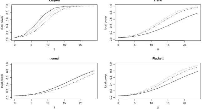
Fig. 1. Asymptotic local power functions of the tests based onσˆ2
n(solid line),T3,4,5,n(dashed line) andTn(dotted line) whenCis the Gumbel–Hougaard copula withτ=0.25 andDis either the Clayton, Frank, normal or Plackett copula withτ=0.25.
As in Section2, the statisticsTδ,(1m)
, . . . ,
Tδ,(Nm)can be thought of as approximate independent realizations ofT, whereTis the weak limit ofTnunder(
Hδn)
n≥1. It is thus natural to estimate the asymptotic critical value ofTnof levelα
as the empirical quantile ofT0(,1m), . . . ,
T0(N,m)of order 1−
α
. We will denote it byqˆ
T(α)
as we continue. The limiting local power function can then be estimated asˆ
β
T(α, δ)
=
1 N NX
k=1 1n
Tδ,(km)≥ ˆ
qT(α)
o
.
The limiting local powers to be represented in the forthcoming graphs were estimated usingm
=
2500 andN=
10 000. A similar approach was used to compute the asymptotic local power function of the test of extreme-value dependence proposed in [19] and based on the statisticT3,4,5,n. For the test based onσ
ˆ
n2, the limiting local power function was computed using the expression given in [1, Proposition 3] in whichµ
0(
0)
was estimated by Monte Carlo integration from samplesof size 500 000, and
σ (
0)
was estimated using the large-sample variance estimator defined in [1, Section 4] from 2500 observations fromC. The last step was performed using code generously provided by Johanna Nešlehová and now available in the R packagecopula
.Asymptotic local power calculations were performed in the following settings:Cwas taken to be the Gumbel–Hougaard copula with
τ
=
0.
25, 0.5 or 0.75, andDwas either the Clayton, Frank, normal or Plackett copula withτ
=
0.
25, 0.5 or 0.75. For the sake of clarity, we only report the results whenCandDhave the same degree of dependence.As can be seen fromFigs. 1–3, the results are consistent with those obtained in the simulations. Local powers increase in all settings as
τ
increases and, for a givenτ
, the greatest local powers are obtained whenDis the Clayton copula. In the latter case, the test based onσ
ˆ
2n slightly outperforms its competitors when
τ
=
0.
25 and 0.5. Whenτ
=
0.
75, all three tests are very close. The test based onσ
ˆ
n2is also more powerful then its competitors, overall, whenDis the normal copula, the difference in local power being more pronounced for higher dependence. WhenDis the Frank or the Plackett copula, the test based onTnis the most powerful and the test based onT3,4,5,nis second best.5. Concluding remarks
Among the various tests of bivariate extreme-value dependence considered in this work, no single test was found to be consistently better than the others. The test proposed in [1] based on
σ
ˆ
2nappears to be better suited for elliptical alternatives, while for the other alternatives considered in the experiments, the testsT
ˆ
An andT3,4,5,nhave the highest rejection rates. Overall, the testT
ˆ
An displays the best behavior. From a computational perspective, the test based on
σ
ˆ
n2is the fastest; it is followed by the tests based onT3,4,5,n,Tˆ
nCand finallyTˆ
nA.Based on the Monte Carlo experiments and local power comparisons presented in this work, our recommendations are as follows. We suggest the use of the testT
ˆ
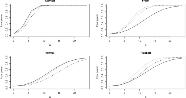
nAin the case of small samples. Whennreaches 400, a faster yet almost as powerfulFig. 2. Asymptotic local power functions of the tests based onσˆ2
n(solid line),T3,4,5,n(dashed line) andTn(dotted line) whenCis the Gumbel–Hougaard copula withτ=0.5 andDis either the Clayton, Frank, normal or Plackett copula withτ=0.5.
Fig. 3. Asymptotic local power functions of the tests based onσˆ2
n(solid line),T3,4,5,n(dashed line) andTn(dotted line) whenCis the Gumbel–Hougaard copula withτ=0.75 andDis either the Clayton, Frank, normal or Plackett copula withτ=0.75.
alternative is the testT
ˆ
nCbased on the expressions given in Section2.6. If one suspects that the dependence might be elliptical or in the case of very large samples, the test based onσ
ˆ
2n should be preferred.
Acknowledgments
The authors are very grateful to Johanna Nešlehová for providing R routines implementing the test based on
σ
ˆ
2 n, and to Mark Holmes for fruitful discussions, as always. The study of the finite-sample performance of the tests was carried out on a Beowulf cluster at the Department of Statistics, University of Connecticut, which was partially supported by NSF grant 0723557 ‘‘Scientific Computing Research Environments for the Mathematical Sciences’’ (SCREMS).Appendix A. Proof ofProposition 1
Proof. Setting
δ
=
0 in(13), we have fromProposition 4that√
n(
Cn−
C)
√
n(
An,c−
A)
; C Ain
`
∞(
[
0,
1]
2)
⊗
C(
[
0,
1]
)
. Letϑ
be the map fromC(
[
0,
1]
)
to`
∞(
[
a,
b]
2)
defined byϑ(
B)(
u, v)
=
exp log(
uv)
B log(v)
log(
uv)
,
B∈
C(
[
0,
1]
), (
u, v)
∈ [
a,
b]
2.
Now, letB
∈
C(
[
0,
1]
)
, let(
tn)
n≥1be a sequence of reals converging to 0 and let(
hn)
n≥1be a sequence of functions in C(
[
0,
1]
)
converging toh∈
C(
[
0,
1]
)
. Then, asntends to infinity and uniformly in(
u, v)
∈ [
a,
b]
2,1 tn
{
ϑ(
B+
tnhn)(
u, v)
−
ϑ(
B)(
u, v)
}
=
exp log(
uv)
B log(v)
log(
uv)
1 tn exp log(
uv)
tnhn log(v)
log(
uv)
−
1→
exp log(
uv)
B log(v)
log(
uv)
log(
uv)
h log(v)
log(
uv)
=
ϑ
B0(
h)(
u, v).
It is easy to verify that the map
ϑ
B0is continuous with respect to the topologies of uniform convergence onC(
[
0,
1]
)
and`
∞(
[
a,
b]
2)
, and linear. It follows thatϑ
is Hadamard-differentiable tangentially toC(
[
0,
1]
)
; see e.g. [32, Chapter 3.9]. From the functional version of Slutsky’s theorem, we then have that√
n{
Cn(
u, v)
−
C(
u, v)
}
√
n{
ϑ(
An,c)
−
ϑ(
A)
}
; C(
u, v)
ϑ
0 A(
A)
in
`
∞(
[
a,
b]
2)
⊗2. The continuous mapping theorem then implies that√
n{
Cn(
u, v)
−
C(
u, v)
} −
√
n exp log(
uv)
An,c log(v)
log(
uv)
−
exp log(
uv)
A log(v)
log(
uv)
converges in`
∞(
[
a,
b]
2)
to(5). UnderH0, representation(1)immediately implies that this is also the weak limit of the test processDndefined in(4).
Appendix B. Proof ofProposition 2
Proof. Let
(
Ui,
Vi)
=
(
F(
Xi),
G(
Yi))
for all i∈ {
1, . . . ,
n}
, letC¯
nbe the empirical c.d.f. computed from the unobservable random sample(
U1,
V1), . . . , (
Un,
Vn)
, and letα
n=
√
n
(
C¯
n−
C)
. Furthermore, following [14], let E= {
(
u, v)
∈ [
0,
1]
2:
0<
u∧
v <
1} =
(
0,
1]
2\ {
(
1,
1)
}
,
let
ω
∈
(
0,
1/
2)
, letqω(
t)
=
tω(
1−
t)
ω,t∈ [
0,
1]
, and letGn,ω
(
u, v)
=
α
n(
u, v)
qω(
u∧
v)
if(
u, v)
∈
E,
0 ifu=
0 orv
=
0 or(
u, v)
=
(
1,
1).
(B.1)From [14, Theorem G.1], we known that the processGn,ωconverges weakly in
`
∞(
[
0,
1]
2)
to a centered Gaussian process Gωwith continuous sample paths.Now, for anyk
∈ {
1, . . . ,
N}
and anyu, v
∈ [
0,
1]
, defineG(nk,ω)
(
u, v)
=
1√
n nX
i=1(
Zi(k)− ¯
Z(k))
1(
Ui,n≤
u,
Vi,n≤
v)
qω(
u∧
v)
=
α
(k) n(
u, v)
qω(
u∧
v)
if(
u, v)
∈
E,
0 if(
u, v)
∈ [
0,
1]
2\
E,
where
α
n(k)is defined in(6). From Lemma 2 of [21], we have that Gn,ω,
G(n1,ω), . . . ,
G(N)
n,ω
; Gω
![As can be seen from [12, Figure 3], the function A C appears convex for the most frequently used bivariate copulas with positive dependence such as the Clayton, Frank, normal and Plackett](https://thumb-us.123doks.com/thumbv2/123dok_us/11089450.2996141/6.816.60.682.746.1029/figure-function-frequently-bivariate-positive-dependence-clayton-plackett.webp)