Three Essays on Financial Economics

(1)

Three Essays on Financial Economics

Kunal Sachdeva

Submitted in partial fulfillment of the requirements for the degree of

Doctor of Philosophy under the Executive Committee of the Graduate School of Arts and Sciences

COLUMBIA UNIVERSITY 2018

(2)

(3)

ABSTRACT

Three Essays on Financial Economics Kunal Sachdeva

This dissertation presents three essays in financial economics. The essays discuss how market frictions can affect outcomes in the real economy, the returns earned by investors, and the investment decisions made by asset managers. The first essay stud-ies how the liquidity of assets can affect outcomes in the real economy. In particular, it focuses on the life settlement market to show how increased liquidity of life insurance contracts are causally linked to greater life longevity. The second essay studies how inside investments relate to managerial compensation and fund performance. The essay focuses on the decreasing returns to scale to arbitrage strategies and the profit maximizing motive of asset managers as the central friction affecting return. The final essay analyzes the role that information acquisition and communication have on the choice to be a principal, agent, or both. The results emphasize how the choice to be either a principal or an agent strictly dominate the mixed strategy of being both, in a highly generalized model.

(4)

(5)

List of Tables

1.1 Summary Statistics, Policy and Policyholder . . . 49

1.2 Summary Statistics, Baseline Covariates and Dependent Variables . . . . 50

1.3 First-Stage of 2SRI, Health Fragility Analysis . . . 51

1.4 Second-Stage of 2SRI, Health Fragility Analysis . . . 52

1.5 Settlement and Disease . . . 53

1.6 First-Stage of 2SRI, Distance to Nearest Hospital Analysis . . . 54

1.7 Second-Stage, Distance to Nearest Hospital . . . 55

1.8 Liquidity of Wealth and Longevity . . . 56

1.9 Robustness Tests . . . 57

2.1 Top 10 Hedge Fund Manager Paychecks, 2016 . . . 100

2.2 Summary Statistics: ADV Data . . . 101

2.3 Summary Statistics: Merged Data . . . 102

2.4 Related Party Information . . . 103

2.5 Inside Investment and Excess Return—Value-Weighted . . . 104

2.6 Inside Investment and Excess Return—Equal-Weighted . . . 105

2.7 Cuts by Fund Size . . . 106

(9)

2.9 Inside Investment and Fund Size . . . 107

2.10 Fund Flows and Performance . . . 108

2.11 Firm-Level Equity Ownership and Returns . . . 109

2.12 Inside Investment and Hedge Fund Fees . . . 110

3.1 Important Notation and Definitions . . . 143

1 Proportionality Tests . . . 170

(10)

List of Figures

1.1 Cashflows Associated with Life Settlement Transactions . . . 22

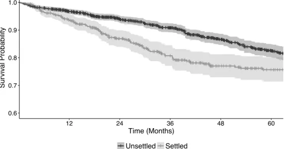
1.2 Survival Curves, Stratified on Settlement Status . . . 42

1.3 Drop in the Financial Strength Rating Through the Great Recession . . 43

1.4 Randomization Check, Regression Coeﬃcients . . . 44

1.5 Motivation for Hazard Model, Right Censoring of Mortality Events . . . 45

1.6 Plot of Life Expectancy Estimates and Age . . . 46

1.7 Geographic Diversity of Observations . . . 47

1.8 Access to the Nearest Hospital . . . 48

2.1 Anecdotal Evidence, Relating Performance to Insider Investment . . . 88

2.2 Heterogeneity of Insider Investment Across Numerous Funds . . . 89

2.3 Firm and Fund Analysis . . . 90

2.4 Sample Form ADV — Renaissance Technologies . . . 91

2.5 Bias Analysis of Merged Sample . . . 92

2.6 Distribution of Insider Investment from Merged Sample . . . 93

2.7 Flow Performance of Funds by Insider Status . . . 94

2.8 Return Predictability Funds by Insider Status . . . 95

(11)

2.10 Quantile Regression of Inside Investment on Excess Returns . . . 97

2.11 Event Study, Transition From One Fund to Multiple Funds . . . 98

2.12 Firm-Level Equity Ownership . . . 99

3.1 Sequence of events . . . 124

3.2 Example of an Interval Equilibrium . . . 144

3.3 Incentive Boundary for Truthful Communication . . . 145

1 Economic Relevance of the Financial Strength Rating . . . 167

2 Description of Data . . . 168

3 Aggregation of Life Expectancy Estimates . . . 169

4 Impairment as a Measure of Fragility . . . 175

5 Gross Return Profiles of Diﬀerent Strategies . . . 186

6 Capital and Payoﬀs . . . 187

7 Payoﬀs to Insider and Components . . . 188

(12)

(13)

Acknowledgements

I owe thanks to countless faculty members, staﬀ members, fellow students, and friends. While I am unable to list everyone here, please know that I am grateful for your help and guidance in completing this dissertation.

I owe gratitude towards my advisors, Profs. Wei Jiang, Kent Daniel, Stephen Zeldes, Xavier Giroud, and Arpit Gupta. I have been privileged to have advisors that have aﬀorded me the intellectual freedom to explore and discover my passion in research.

I am thankful to my friends, and in particular, Pablo Slutzky and Ye Li. Their friendship has been important in carrying me through my time at Columbia Univer-sity.

I am thankful to have met Jon Mendelsohn, Jason Mendelsohn, and the entire Ashar Group. Their friendship, help, and belief in my research has been important to the completion of this dissertation.

I am deeply indebted to my family for their love. To my parents, Reeta and Rajinder Sachdeva, to whom this dissertation is dedicated. To my sisters, Jasmine and Natasha Sachdeva, and their husbands, Zdenko Popovic and Rahul Brahmbhatt, for their unwavering confidence in me throughout my years in graduate school.

Lastly, I thank Stephanie Lau. Without her constant support and encouragement, this dissertation could not have been completed.

(14)

(15)

Dedicated to my beloved parents

Reeta Sachdeva and Rajinder Sachdeva

(16)

(17)

Chapter 1

Liquidity and Longevity,

Bequest Adjustments Through the Life

Settlement Market

∗

Kunal Sachdeva‡

Access to wealth is vital for our rapidly aging population. This paper studies the financial decisions of individuals nearing their end of life and examines if access to such wealth can enable longevity. I use transaction-level data from the secondary market for life insurance policies, also known as the life settlement market. In this quasi-experimental evaluation of bequest adjustments, I show that the ability to access wealth through the life settlement market leads to a significant increase in longevity. This eﬀect is stronger for people in fragile health, with severe disease diagnoses, and those with limited access to hospitals. The regional supply of primary healthcare, and the social-economic background of the policyholder does not seem to explain the longevity eﬀect. Taken together, these results appear to be related to the high-cost of care for individuals and the importance of financial liquidity for people nearing their end of life.

∗I am grateful to my dissertation committee members: Wei Jiang, Kent Daniel, Stephen Zeldes,

and Xavier Giroud for their valuable suggestions and support. I also thank Simona Abis, Tania Babina, Emily Breza, Pierre-André Chiappori, Olivier Darmouni, John Donaldson, Jason Don-aldson, Arpit Gupta, Andrew Hertzberg, Gur Huberman, Amit Khandelwal, Giorgia Piacentino, Tomasz Piskorski, Stijn Van Nieuwerburgh and the seminar participants at the Canadian Eco-nomic Association (2016), Columbia Business School, Rochester (Simon), Dartmouth (Tuck), UBC (Sauder), Ohio (Fisher), LSU (Ourso), Florida (Warrington), Toronto (Rotman), CityUHK, CUHK, NTU, NUS, Vanderbilt (Owen), and Rice (Jones) for helpful comments. A.M. Best owns the copy-right to their data and I use with permission. Finally, I am indebted to Jon Mendelsohn and Jason Mendelsohn of Ashar Group, both for their market insight support through this paper. Views ex-pressed in this paper are those of the author, and do not necessarily reflect the opinions of anyone else. All results have been reviewed to ensure that no confidential information is disclosed. Columbia University and The Chazen Institute at Columbia provided critical funding to support this research.

(18)

1.1 Introduction

The United States is facing an unprecedented challenge in funding its rapidly aging population.1 _{In order to address this need, seniors have utilized annuities, reverse}

mortgages, and the proceeds from selling personal assets to fund their consumption. Indeed, a recent study of people nearing their end of life found wealth to be an important consideration for out-of-pocket expenditures, with the average household spending $11,618 during their last year of life.2 _{Previous papers have emphasized}

that inadequate resources can aﬀect life longevity. However, there still remains the question if, and how, the accessibility of one’s wealth, especially nearing one’s end of life, can aﬀect longevity?

This paper presents a quasi-experimental evaluation of the liquidity of wealth for individuals nearing their end of life. The paper finds that the financial liquidity of one’s bequest allocation has a statistically significant and economically large eﬀect on longevity. Studying the possible mechanisms by which the accessibility of wealth relates to longevity, this paper documents that gains are accruing to individuals in fragile health, with severe disease diagnoses and limited access to healthcare. These results appear to be related to the high-cost of care for individuals and the importance of financial liquidity for people nearing their end of life. Lastly, this paper provides further evidence that shocks in the financial sector are both important and can have unintended spillover eﬀects into the real economy.

It is diﬃcult to study the eﬀects of the accessibility of wealth on longevity. In developed countries, health insurance, education about basic nutrition, and the ex-istence of social infrastructure makes the relation between wealth and longevity less

1_{From the US Census Bureau: "In 2050, the population aged 65 and over is projected to be} 83.7 million, almost double its estimated population of 43.1 million in 2012." See Ortman, Velkoﬀ, Hogan, et al. 2014.

2_{See Marshall, McGarry, and Skinner 2011, spending in the last year of life is is skewed, with} the 90th percentile equal to $29,335.

(19)

plausible. Further, assuming that a relationship does exists, there are numerous channels by which wealth influences longevity. This makes the inference of a causal relationship diﬃcult.3 _{Ideally, a randomized trial would provide the conditions to}

iso-late the eﬀects that wealth has on individual-level mortality. However, for developed countries like the United States, implementing such a trial is highly cost-prohibitive.4

This paper solves this data challenge by using a proprietary dataset that is particu-larly well suited to study the liquidity of wealth on longevity: the sale of life insurance contracts by policyholders to investors in the secondary market, also known as the life settlement market. Life settlement transactions are typically large lump-sum bequest adjustments for individuals nearing their end of life. As such, data from this market makes an ideal setting to test both if and how the accessibility of wealth enables longevity. The data used in this paper comes from a leading life settlement broker in the United States, with the data representing $4.5 billion in death benefits from 2009 to 2017.5

Naturally, the main econometric challenge in causally estimating how wealth af-fects longevity stems from the issue of reflexivity and endogenous choice, Manski 1993. In this paper’s setting, individuals who sell their policy die sooner than those who do not, as seen by the stratification in Figure 1.2. This observation could lead to the misleading inference that capital providers are contributing to these policyhold-ers’ deaths, or that they are advantageously selecting distressed policyholders in the secondary market. Even if the econometrician controls for individual level health, a longer observed life following the sale of one’s life insurance policy is not suﬃcient

3_{From one perspective, wealth enables an individual to live longer through the routine} consump-tion of healthier foods, better healthcare, and safer housing as compared to less wealthy individuals. Alternatively, an individual may have private information and know that they are likely to live longer than their average population, and thus rationally accumulates wealth to better smooth their lifetime consumption.

4_{Researchers have instead relied on quasi-experimental settings to study this relationship.} 5_{The data used in this paper is a subsample of all transactions executed by the broker. A} discussion of this can be found in Appendix 3.8.

(20)

evidence to claim that wealth contributes to longevity.6 _{Thus, understanding the}

causal contribution of how wealth aﬀects longevity has proven to be diﬃcult.

This paper addresses these identification challenges by focusing on a quasi-experimental shock through the Great Recession that reduced and often eliminated the ability of policyholders to reallocate their wealth from the future to the present: the re-pricing of counterparty risk of life insurance companies and their associated policies in the secondary market. Prior to the Great Recession, insurance companies were generally thought to be safe, long-lived institutions. However, as the Great Re-cession unfolded, this assumption was challenged, with many insurance companies’ financial strength rating downgraded to reflect the increased probability of impair-ment at the insurance-company level. Due to the uniqueness in how life insurance policies are priced, the shock to the financial strength rating reduced or eliminated the desirability of a life insurance policy from the perspective of an investor.7 _{I use this}

heterogenous shock to insurance companies’ financial strength rating to instrument for the liquidity of wealth through the secondary market.

Using a Cox proportional hazards model in a control function specification, I estimate the relationship between the accessibility of wealth to an individuals life longevity. The analysis is made between individuals who both approach a broker, where one group is able to complete a settlement while another is not. The primary dependent variable is life longevity, as measured by the number of months lived post-settlement. The main explanatory variable is observed sale, or settlement, of the policy. Due to the possible endogeneity in observing a settlement, I instrument this

6_{A longer observed life could be attributed to other channel, such as adverse selection in the} secondary market, or unobservable health diﬀerences.

7_{This is driven by two features that are unique to life insurance policies: First, the cost of} insurance for a universal life policy is negative and typically growing over time. Thus, a small reduction in the expected death-benefit can greatly reduce the valueness of a policy, resulting in a negative price. Second, the participation constraint of a policyholder is at least zero dollars. All policies have a costless abandonment option through lapsation. Because a policyholder can freely walk away from a contract by suspending all future premium payments, a negative price would not be supported in this market.

(21)

variable using the financial strength rating, or rating, of the insurance company at settlement. The null hypothesis is that policyholders who are able to sell their policy can live longer, as compared with the individuals that don’t sell their policy.

Armed with a plausibly exogenous instrument, I am able to attribute if the liquid-ity of wealth can enable longevliquid-ity. The first-stage estimate suggests that the financial strength rating of the insurance carrier positively relates to the observed sale of an insurance policy. These results are economically and statistically important, with a single level downgrade in the companies rating relating to a 5.2% decrease in marginal contribution to sell a policy. This suggests that investors are not just concerned about the longevity risk of an individual policyholder, but also the counterparty risk of an insurance company.8

From the paper’s preferred baseline specification, the second-stage estimate shows that the liquidity of wealth positively relates to longevity. Using a hazard model to es-timate longevity, the accessibility of wealth decreases baseline hazard rate by roughly

30W. Estimating the gain to longevity from standard actuarial tables, an 80 year

old, non-smoking male in sub-standard health would gain roughly nine months in life expectancy. The sign and magnitude are plausible in context of the hazards model, as the baseline sample of the study is comprised of older and sicker individuals. The av-erage age of the sample is 79 years, with a majority coming from sub-standard health background.9 _{To further validate these results, the paper implements a standard}

two-stage least squared approach and finds a similar longevity result.

Having shown that the liquidity of wealth causally relates to longevity, the pa-per conducts four separate tests to pin down the mechanism by which the gains to longevity are accruing policyholders. The paper first explores how the gains to longevity works through the health channel by considering the treatment eﬀect to

in-8_{This is further validated by consulting market participants.}

9_{To provide context, aging by just one year in this estimate increases the hazard rate by roughly}

(22)

dividuals from more fragile age-adjusted health as compared to individuals in perfect health. This test is motivated by the range and natural upper limit to life expectancy, as illustrated in Figure 1.6.

Consider Jane Doe (censored identity) who initially purchased life insurance at the age of 47 to provide security for her family. Unfortunately, she was diagnosed with cancer and decided to sell her policy at the age of 61. With the net death benefit amount of the policy over $130,000, she settled her policy for $75,000 in proceeds. In a testimonial, Jane Doe’s husband said:

“These funds will be life changing as we battle for my wife’s prolonged time with us....these funds will help ease that work in ways we haven’t begun to imagine, beyond only paying treatment expenses as we hold out for the next targeted therapy to hit the market, at some astronomical price?”

For people like Jane Doe, selling her policy in the secondary market may have enabled her to consume wealth to extend her longevity.10 _{The paper tests the}

hypoth-esis that the treatment eﬀects are accruing to individuals with more fragile health conditions by splitting the dataset on health fragility and re-examining the eﬀect of liquidity on longevity.

The results of this test suggest that the improvements to longevity are primarily driven by the fragile health subsample, with improvements of roughly 50W from

baseline hazard rates.11 _{Interpreting this result, the sign and magnitude are plausible}

in context of the hazards model, as the baseline sample is comprised of individuals that are old and with severe health conditions. When testing the converse, individuals

10_{Many other anecdotal examples illustrate the possible link between current wealth and health.} An recent example from Dr. Saltz at the American Society of Clinical Oncology Annual Meeting discusses the current per-mg costs of drugs: $28.78 for nivolumab and $157.46 for ipilimumab; pembrolizumab (Keytruda), costs $51.79/mg. "As a clinician, I want these drugs and others like them to be available for my patients. As one who worries how we will make them available and minimize disparities, I have a major problem—and that is that these drugs cost too much. ... To put that into perspective, that’s approximately 4000 times the cost of gold", Helwick 2015.

11_{Estimating the gain from standard actuarial tables, an 80 year old, non-smoking male in poor} health would gain nearly 18 months in life expectancy.

(23)

in mild to perfect health, there are no measurable gains to treatment. Instead, only well known observables such as health status, level of death benefit, and how seasoned a policy is predict longevity outcomes.

The second test considers if the treatment has heterogenous eﬀects on longevity based on an individual’s primary medical diagnoses. It is hypothesized that it is unlikely that all medical diagnoses are equally aﬀected by the treatment of wealth, and as such, gains in longevity are concentrated among certain types of ailments. Interacting settlement status with diseases, the paper finds that health improvements are primarily concentrated among individuals with severe diagnoses. This result is consistent with the previously mentioned fragility test and anecdotal evidence from discussions with several capital providers in the life settlement market.

The third test considers how the accessibility to hospitals relate to longevity.12 _It

is possible that the individual distance or time to the nearest hospital is an impor-tant, but omitted, variables that are predictive of longevity.13 _{Further, it is posited}

that policyholders may be able to use their wealth to move closer to a hospital in an eﬀort to access healthcare and aﬀect their longevity.14 _{To investigate this}

pos-sibility, the paper uses geocoded data to measure the distance and travel time to the nearest hospital for each policyholder. Using these new measures in the baseline specification the paper uncovers that there exists a positive, yet weak, relationship between distance and mortality. More interestingly, when splitting the data based on distance, the paper finds that the treatment eﬀect is more important for individuals living further from a hospital. The results provide evidence that access to wealth is plausibly important for individuals with poorer access to healthcare.

12_{This possibility was raised in a conversation with an institutional investor in life settlement} assets.

13_{In the baseline regression, county level healthcare supply does not relate to longevity. However,} the lack of a result may be driven by averaging individual distances at the county level.

14_{The paper would ideally use a panel data on housing. However, at this point, it is not able to} access this data.

(24)

The fourth test considers how the liquidity of wealth interacts with the financial background of policyholders. It is hypothesized that the benefits of selling one’s policy aﬀects policyholders diﬀerently, either based on their current financial position or their social-economic background. Ideally, an econometrician would be able to observe panel data for each policyholder. To this end, this paper is currently merging against panel data of credit and consumption. However, at the time of writing this, the merge and analysis is not complete. This paper instead uses proxies of wealth, such as the the policyholders social-economic background as inferred by the United States Census data, to measure wealth. Using the median tract level income of each policyholder in the baseline regression,15 _{the paper does not find a relationship}

between social-economic background and longevity. While this specification may be averaging the heterogeneity at the tract level, it is suggestive that the social-economic background of the policyholder isn’t a significant driver of the main results.

To complement the previous analysis, the paper conducts several robustness tests to rule out alternative explanations that have been suggested — other than liquidity — to be driving the results. As a first test, the paper includes additional covariates that have been suggested as important in the selection of policies. As a second test, the paper investigates the possibility that the longevity result is driven by the life expectancy aggregation method. As a final test, the paper conducts a placebo test to rule out the possibility that the baseline results are driven by spurious correlations. The results of the robustness tests are consistent with the baseline results in the paper.

These results improve on previous research by addressing many of its data and em-pirical limitations. First, previous research has relied on subjective health measures, which typically contain well-known biases in reported health status.16 _{In contrast,}

15_{Tract is a small geographical unit, with a population size between 1,200 and 8,000 people, and} an optimum size of 4,000 people.

(25)

this paper relies on a rich dataset of objective life expectancy estimates from special-ized underwriters which is free of biases found in subjective health measures. Second, other papers have used data from life settlement transactions from a single investor or underwriter, but this may be subject to firm level biases that limit the extendability of their results. Instead, this paper has the unique advantage of using broker-level data that is free of the inherent selection bias driven by an investor’s preferences and strategy.

While this paper emphasizes the importance that the liquidity of wealth has on longevity and the possible mechanisms for these gains, the results also come with numerous caveats that should be mentioned. First, the paper is unable to account for the possibly important inter-generational eﬀects of wealth.17 _{However, previous}

studies have suggested that such intergenerational eﬀects are negligible or small.18

Second, the sample of individuals in this paper are wealthier than the average popu-lation in the United States, which may limit the extendability of the results. Although the results are based on a selective sample, the eﬀects are postulated to be larger for individuals from poorer and more financially constrained backgrounds. Third, the paper focuses on the secondary market for life insurance policies which may limit the extendability of results. While the secondary market is relatively small, the total market size of the life insurance industry is $20.8 trillion of policies in-force,19 _{and has}

an ownership rate of 70%.20 _{These facts suggest that the paper is both extendable}

and important, especially given the rapidly aging population.

due to the substitutability of wealth and health. An example comes from smoking, where can improve mental health while being harmful to one’s health.

17_{It is posited that the potential wealth benefits to the current generation may come at the expense} of future generations welfare.

18_{See papers such as Meer, Miller, and Rosen 2003; Kim and Ruhm 2012; and Carman 2013,} which have studied the aﬀect of inheritances using PSID and HRS data.

19_{See ACLI 2016.}

20_{See LIMRA 2014 for the market size of the life insurance industry. In comparison, see Mankiw} and Zeldes 1991 for the household ownership of stocks.

(26)

In light of these caveats, this paper makes five important contributions. First, it uncovers an important friction that limits the liquidity of life insurance policies in the secondary market: the counterparty risk of insurance companies as measured by the financial stability rating. Second, the paper overcomes both data and sample selection problems of previous research, to uncover a new and important gradient by which wealth can affect health: the liquidity of wealth for individuals nearing their end of life. Third, the paper documents that gains are accruing to individuals in fragile health and with severe disease diagnoses. Fourth, the paper presents evidence against channels such as regional supply of healthcare and social-economic background to be driving the results. Fifth, this paper shows that spillover effects of financial risk of an institution can have real, and large effects on one’s longevity.

The paper proceeds as follows. Section 1.2 outlines the contribution of this paper makes to several strands of literature. Section 1.3 provides necessary institutional details, outlines the data, and methodology used in this paper. Section 1.4 outlines the censoring issue with mortality data and discusses the instrumental variable ap-proach. Section 1.5 presents causal evidence that the liquidity of wealth relates to longevity. Section 1.6 explores the possible mechanisms driving these results. Section 1.7 presents robustness tests. Section 1.8 concludes.

1.2 Contribution to Literature

This paper contributes to several strands of literature. It first contributes to the literature linking the eﬀects of wealth shocks on health outcomes.21 _{This literature}

has studied numerous channels by which wealth shocks can eﬀect health outcomes, including but not limited to, debt forgiveness (Dobbie and Song 2015), lottery

win-21_{The relationship goes both ways, with health shocks also aﬀecting economic factors: For} ex-ample, unanticipated health care expenditures and personal bankruptcies Himmelstein et al. 2005, household borrowing and expansion in number of credit cards Gupta et al. 2015, medicaid expansion and the associated reduction of individual level bankruptcy Gross and Notowidigdo 2011.

(27)

nings (Apouey and Clark 2015; Cesarini et al. 2016; Gardner and Oswald 2007; Lin-dahl 2005), job displacement (Sullivan and Von Wachter 2009), inheritance (Carman 2013; Kim and Ruhm 2012; Meer, Miller, and Rosen 2003), stock market fluctuation (Engelberg and Parsons 2016; Schwandt 2014), and housing and foreclosures (Cur-rie and Tekin 2015; Fichera and Gathergood 2016). Other studies have focused on quasi-experiments from emerging markets including, pensions (Case 2004; Jensen and Richter 2004), and economic improvements through German reunification (Frijters, Haisken-DeNew, and Shields 2004). However, to the author’s knowledge, this is the first paper in this literature studying the liquidity of wealth, for individuals nearing their end of life, and its possible eﬀects on longevity.

This paper also contributes to the literature studying the life settlement market. Papers have studied the equilibrium implications of the life settlement market (Daily, Hendel, and Lizzeri 2008; Fang and Kung 2010a; Hendel and Lizzeri 2003). Other papers have considered the welfare implications of this market (Fang and Kung 2010b; Fang and Wu 2017). The closest papers to this are Januário and Naik 2014, and Bauer, Russ, and Zhu 2014. These papers have studied the null of adverse selection in the life settlement market. In contrast, this paper proposes a possible hidden action story, where individuals can aﬀected their health through accessing their wealth. This paper also diﬀerentiates itself by overcoming selection issues driven by specific market participants.

Lastly, this paper relates to the literature studying the relationship between social economic status (SES) and longevity. It is a well known fact that individuals from better SES live longer, as shown in recent papers by Bosworth, Burtless, and Zhang 2016, and Chetty et al. 2016. This result is robust to many other settings, including but not limited to, social security data in Snyder and Evans 2006, Census and NCHS data in Lynch et al. 1998, English survey data in Adda, Banks, and Von Gaudecker 2009, and the Whitehall study of British civil servants in Marmot et al. 1991. While

(28)

this correlation persists between measures of income and longevity, there is no consen-sus of the mechanisms driving this result (Cutler, Deaton, and Lleras-Muney 2006). This paper makes a contribution to the broad literature studying SES on longevity by investigating factors such as regional supply of healthcare, distance to hospitals, and social-economic background of the policyholder’s neighborhood.

1.3 Institutional Setting and Data

There are three main challenges in causally estimating the eﬀects of wealth on an individual’s longevity. First, in a developed country, it is important to find an ap-propriate sub-population where such an eﬀect could be plausibly important and em-pirically measurable.22 _{Second, the treatment size would need to be large enough to}

be empirically measurable. Reallocating a small amount of wealth would not plau-sibly aﬀect longevity. Third, relating bequest reallocations to longevity suﬀers from the issue of reflexivity and endogenous choice, Manski 1993. Observing a positive correlation between individuals who sell their policy and ex-post longevity is equally consistent with individuals being more attentive to their health and with individuals having superior knowledge of their longevity.

This paper overcomes these three challenges by focusing on a quasi-experimental setting and novel dataset from the secondary market for life insurance policies. First, individuals who can access this market are nearing the end of their lives, have a median sample age of 79 years, and are often of sub-standard health, as shown in Table 1.1. Second, the reallocation amount is substantial, with the gross median settlement value of $235 thousand dollars, and thus plausibly large enough to matter. Third, the dataset is for the post-crisis period of 2008 and exploits a market feature

22_{This paper posits that any wealth eﬀect would most likely be important for older individuals,} nearing their end of life, and in poorer health.

(29)

that aﬀects the desirability of policies, that are plausibly exogenous to longevity, other than its eﬀect on liquidity of a policy.

The following subsection presents institutional details about the life settlement market and the data used in this paper.

Institutional Setting

Introduction to Life Settlements

Life insurance policies can be characterized as mortality-contingent contracts that pay a pre-defined benefit when the insured individual dies. Policyholders pay premiums on a periodic schedule to an insurance company and in exchange, in the event of the policyholder’s death, the insurance company pays the policyholder’s beneficiary a death benefit.23 _{This contract can be thought of as a continuation option, as}

the contract terms are determined ex-ante and typically in nominal terms, but the policyholder learns about health as they continue to pay for the policy’s coverage.24

A policyholder may decide to discontinue their coverage prior to their death.25 _A

policyholder has several options if they choose to dispose of their coverage. The first and most common option is to allow their policy to lapse by suspending payments on premiums.26 _{Alternatively, a second option, policyholders may put their policy}

back to their insurance carrier. In exchange, the policyholder receives an immediate,

23_{Premiums tend to be front loaded, with policies at origination typically resulting in a negative} NPV at any non-negative discount rate Cawley and Philipson 1999. This is done to ensure a pooling equilibrium.

24_{Life insurance policies have been characterized as a contract with one-sided commitment with} learning, Hendel and Lizzeri 2003. This is a adaptation of Harris and Holmstrom 1982.

25_{This can be driven in part by learning, where one discovers positive improvements to their health,} in eﬀect rendering the policy worthless. Alternatively, it can also be motivated by background risk such as a change in bequest motive, or even a financial constraint, where a policyholder can no longer fund the periodic premiums.

26_{Previous research has empirically shown that policyholders adjust, and often reduce, their} cov-erage throughout their life. About 4.2% of all life insurance policies lapse each year, see Gottlieb and Smetters 2014.

(30)

one-time lump-sum, cash payment also called a cash surrender value (CSV). The CSV is often a small fraction of the death benefit and is a function of past premiums paid, policy size, and underwriting classification. Importantly, it is independent of the insured’s health condition at the time of surrender and often de minimus compared to the death benefit. Taken together these options can be expressed asKt(CSV,0),

have a non-negative value and, most importantly, are independent of the insured’s health.

As a third option, and the main empirical observation in this paper, a policyholder can sell their life insurance policy to an investor through the life settlement market.27

The original policyholder would receive a one-time lump-sum payment at the time of sale, and in exchange, the capital provider would assume all future premium pay-ments. Upon death of the original policyholder, the investor would receive the death benefit associated with the policy.

Data

This section discusses major components of the dataset and reasons for inclusion in the next subsections. For brevity, much of the merging information is relegated to the Appendix.

Policy and Insured Data

The primary dataset in this paper comes from a broker in the life settlement market that acts as an intermediary between buyers and sellers.28 _{Hand checked for accuracy,}

the broker-level data is comprised of three main datasets: (i) All Observations, (ii)

27_{See Appendix 3.8 for a brief overview of the life settlement market.}

28_{The broker represents the selling policyholder in these transactions and is incentivized through} a commission schedule to obtain the best price.

(31)

Main Set, and (iii) Settled Data, and summarize in Table 1.1.29 _{Policy data include}

death benefit and level premiums to maturity, while the policyholder data include age and gender.30

Life Expectancy Estimates and Mortality

Life expectancy estimates are pivotal in valuing life insurance policies. This is because the insured’s survival probability is the main source of uncertainty.31 _{Although age}

and gender are good first-order estimates of one’s life expectancy, there can be great heterogeneity at the individual level. To increase the precision of their longevity estimates, insurers typically require individuals to release their medical history, which insurers submit to a third-party underwriter.32 _{The underwriter evaluates the medical}

history to provide an objective estimate of the individual’s survival duration. From these, the paper also calculates an age-gender adjusted measure of health fragility.33

The broker matches the sample of the insured against a third-party death database.34 _{The paper constructs the primary outcome variable used in this paper,}

29_{Although many potential sellers may contact the broker, not all policies or policyholders are} ideal for a life settlement transaction. Thus, the level of detail for each policy and policyholder varies with the level of engagement.

30_{The number of policies and policyholders are not equal, due to joint and multiple policies per} individual.

31_{While longevity is the primary source of risk, the paper acknowledges there are additional} sources of risk. This includes the uncertainty related to the change of cost of insurance (COI) of policies. Further, depending on the funding structure of the assets, there may also be interest rate and funding risk associated with these assets. These are seen as secondary concerns to longevity.

32_{These underwriters are akin to a credit underwriter like Moodys, S&P, and Fitch in the} fixed-income securities market, but instead for medical data.

33_{Using broker level data, this paper observes over 4000 third-party life expectancy with a mean} life expectancy for settled policies of 82 months. An overwhelming majority of estimates come from three leading medical underwriters, see Appendix 3.8. Adjustment are made in the analysis to account for the passage of time between the underwriting and settlement date, see Appendix 3.8.

34_{Enrichment is done to account for the re-interpretation of Section 205r of the Social} Secu-rity Act in November 2011. The Social SecuSecu-rity Death Master File (SSDMF) doesn’t disclose state death records unless these deaths were independently reported to the Social Security Administration through a “First-Party Source”. These are generally family, friends, funeral homes, coroners, hospi-tal, and so forth. More detail about mortality data considerations can be found in the Appendix, Section 3.8.

(32)

life achievement. This measures the amount of time from the last date of contact with the broker (typically the settlement date) to either: (i) their date of death, or (ii) the final date of the study, March 1 2017.

Financial Strength

To establish a measure of financial strength, the paper uses A.M. Best data for its broad coverage, long time series and informational content in its rating. This dataset tracks the insurance carriers’ financial strength rating and forms the basis of my instrument for causal estimation.35 _{The paper translates the letter grade into a linear}

scale ranging from zero to seven, with the best rating corresponding to the highest rating. The resulting dataset was linked to the policy data.

Regional Data

To control for regional-level data, the raw address data was standardized, geocoded, and merged against 11-digit FIPS code. For regional social-economic factors, tract-level FIPS codes were matched against the 2010 Decennial Census dataset to include median household income. To control for regional supply of healthcare, the data was matched against the 2016 County Health Rankings & Roadmaps at the county level. Next, both the individual’s distance and travel time to the nearest hospital were calculated.

1.4 Empirical Strategy

There are two challenges when estimating the causal contribution of wealth accessi-bility to an individual’s life longevity. The first section discusses the issue of right censoring of mortality data and the motivation for using a hazard model. The second

(33)

section outlines the identification strategy used to causally link settlement status to longevity.

Censoring of Mortality Data

The first empirical challenge is the issue of censoring. The event of interest in this paper, death, is not always observed by the end of the study period and thus is right censored. However, there is still valuable information in knowing that they’ve survived until the end of the study period. As such, an empirical strategy should incorporate this information into its estimates.

To be more precise about the empirical challenge, consider Figure 1.5, which illustrates the issue of right censoring. Panel A shows the case in which the longevity period is observed, ∆tA

2. Depending on the ex-ante life expectation, it is clear if the

individual outlived their expectation. In contrast, Panel B shows the more common case: individual surviving through the end of the study, with the longevity period of ∆tB

3 going unobserved. Again, conditional on ex-ante life expectancy estimates,

an unobserved mortality event does not necessarily imply that an individual lived shorter or longer than expected.

Hazard Model

The appropriate estimation method for the available data and question asked is a haz-ard model.36 _{With regards to the mortality events, consider} _P₍_t_{) =} _S`₍_T _≤_t₎ _and

p(t) =dP(t)/dt as the cumulative distribution function and the probability density function, respectively. Then the conditional instantaneous probability risk of mortal-ity at timet, conditional on survival to that time is given byh(t) =p(t) / (1₋P(t)).

This hazard function forms the measured variable of the main analysis.

36_{The following discussion is based on Kiefer 1988, Lancaster 1992, and chapters 17-19 of Cameron} and Trivedi 2005.

(34)

The paper’s preferred structural equation is the Cox proportional hazards model, and is generally expressed as:

hg(t, X) =h0g(t)2tT{β′X} (1.1)

It is among the most popular method due to the flexibility of its baseline hazard function. The econometrician avoids having to make arbitrary, and possibly incorrect, assumptions about the form of the baseline hazard function. The first factor,h0g(t),

is the baseline hazard function, and is left unspecified. The second factor,2tT{β′_X_}

is the shift factor, with the regressors entering linearly. Notice that if the covariate is equal to zero, the shift factor equals one, and does not contribute to the hazard rate. It is called a proportional model because estimated covariates are assumed to aﬀect the baseline hazard rate,h0g(t), across the entire domain of time. This model

can be further estimated by using stratifications g = 1, . . . , k∗. Stratification may be appropriate, as the baseline hazard function, h0g(t), may be diﬀerent for each

stratum specified in an estimation.37

Identification Strategy

The second empirical challenge is the issue of identification. This is because using the observed sale,settlement, of the policy as the main explanatory variable for longevity may be problematic due to the issue of reflexivity and endogenous choice. There are countless stories that could overstate (or understate) the relationship between settlement and longevity. For example, a policyholder may have private and superior

37_{This paper stratifies the sample into terciles based on age and health impairment and verifies the} appropriateness of this assumption by examining the product-moment correlation between the scaled Schoenfeld residuals. The results of these tests are found in Appendix 3.8. Note, the assumption of proportionality should also be tested to ensure appropriateness of the model. This can be done by looking at the product-moment correlation between the scaled Schoenfeld residuals and the time for each regressor.

(35)

information about their health and thus would upward bias an estimate.38 _Conversely,

investors may have a superior ability to infer longevity from medical data and are advantageously selecting policyholders. These and other many possible stories pre-vent the econometrician from making causal statements from a simple correlation. Further, these stories make it unclear in which direction a bias, if any, would exists.

The paper overcomes this challenge by proposing an instrumental variable ap-proach and, in particular, uses the heterogenous shock to the rating of insurance carriers as an instrument for the settlement of an insurance policy. An insurance company’s financial strength rating aﬀects the desirability of a policy as this, in part, aﬀects the counterparty risk of the policy and thus its valueness. Using an instru-ment for settleinstru-ment status allows me to make causal inferences based on the extensive margin of one’s ability to access their wealth.

The following subsections details the instrument, mechanisms by which it oper-ates, the exclusion restriction, and empirical considerations.

Insurance Companies Through the Great Recession

Prior to the Great Recession, insurance companies were thought to be safe, long-lived institutions. However, at the onset of the Great Recession, insurance companies were shown to be systematically important to the financial and real economy, Koijen and Yogo 2016b. Further, the recession challenged the conventional wisdom that the in-surance industry was simply maturity-matching between their assets with liabilities, Chodorow-Reich, Ghent, and Haddad 2016. While the near failure of AIG was well covered in the popular media, it was not the only insurance company that faced fi-nancial distress. As pointed out in Koijen and Yogo 2016a, insurers like AIG was challenged both by their default swaps and security lending, McDonald and Paul-son 2015; Peirce 2014. Several insurance companies applied and received assistance

(36)

Troubled Asset Relief Program (TARP), while others were rejected, or withdrew their application for TARP. Other firms took corporate actions such as cutting dividends or issued equity.

In the event that an insurance company went bankrupt, the underlying policies would be partially guaranteed by state-level co-insurance programs.39 _{While there are}

explicit and implicit guarantees for the policies underwritten by insurance companies, the limits on coverage can materially impact their expected value. These limits are established at the state level, with most states consistently setting limits in line with the NAIC Model Act, provide coverage up to $300,000 in life insurance death benefits.40 _{While this is su}_ﬃ_{cient for policies with a low face value, it would imply}

a possibly large drop in value for any policy of value greater than $300 thousand in death benefit.

Non-Positive Pricing of Insurance Contracts

The increased risk in the insurance industry had real implications for the associated policies that were underwritten by these institutions. The issue can be seen in the equation describing the intrinsic value of a long position in an insurance policy:

E[Vmarket] = ! T ! t=1 ⎧ ⎪ ⎪ ⎪ ⎪ ⎨ ⎪ ⎪ ⎪ ⎪ ⎩ S`(Deatht) F (1 +r)t − t & s=1 {1₋S`(Deaths)} ' () * Survival P robability Pt (1 +r)t ⎫ ⎪ ⎪ ⎪ ⎪ ⎬ ⎪ ⎪ ⎪ ⎪ ⎭ (1.2)

39_{This parallels the federally-mandated insurance for the potential failure of banking (FDIC) and} investing (SIPC), but at the state level and for insurance companies. If an insurance company fails, it is taken over by all other insurance companies at the state level, who honor the claims or transfer them to financially stable insurance institutions. If this is not possible, the failed insurance carrier is taken over by the insurance department of the regulating state.

40_{Note, there are limits for overfunded policies. Often, the limit is up to $100,000 in cash surrender} or withdrawal values for life insurance policies. For more information, see https://www.nolhga.com/.

(37)

where S`(Deaths) is the instantaneous probability of death, t and T. represent

time, and the mortality date of an individual, respectively. TheF is the death benefit to the beneficiary upon the insured’s death. Pt is the minimum premium required for

a given period, and there is no uncertainty in the cashflows.

Given the cashflow structure of equation (1.2), it is often the case that there does not exist a positive expected price for a life insurance policy (See Hendel and Lizzeri 2003).41 _{This uniqueness is driven by two features that are unique to life insurance}

policies: (1) front-loaded premiums and (2) a costless abandonment option.

The front-loaded premiums allows an insurance contract to have negative values for a long position. Unlike a normal financial asset such as a coupon bond, insurance policies must pay premiums until maturity. If, however, there is a reduction in the expected death benefit of an insurance policy, the valueness can be greatly reduced or eliminated, resulting in a negative expected price.

The costless abandonment option prevents negative prices from being supported in the secondary market. Lacking commitment, policyholders can walk away from a contract by suspending all future premium payments. Therefore life insurance policies in the secondary market must have a positive expected price at settlement. Thus, shocks to the financial strength rating can reduce or entirely eliminate the desirability of a life insurance policy from the perspective of an investor.

These two facts together creates a naturally occurring separation between valuable and valueless policies. This is illustrated in Figure 1.1.

Instrumental Variable Analysis

The paper uses this plausibly exogenous shock to the insurance carrier’s financial stability rating as an instrument to estimate the causal contribution of liquidity on

41_{Nearly all life insurance policies are front loaded, Gottlieb and Smetters 2014, and as such, not} all life insurance contracts have positive price. Further this statement is not claiming that the value of the insurance policy is negative for a policyholder, as in fact, it can provide a hedge to the loss of human capital and may be utility improving.

(38)

Alex

Low Risk Company

E[Vn] Pn+1Pn+2 PT!−1

F Bob

High Risk Company

E[Vn] Pn+1Pn+2 PT!−1 F

(A) Policy and Policyholder’s, Pre-crisis

Alex

Low Risk Company

F×πHigh Bob

High Risk Company

E[Vn] Pn+1Pn+2 PT!−1 F×πLow

(B) Counterparty Risk Aﬀects Expected Value

Alex

Low Risk Company

E[Vn] E[Vn] Pn+1Pn+2 PT!−1 F×πHigh excluded Bob

High Risk Company

E[Vn]

E[Vn] Pn+1Pn+2 PT!−1 F×πLow

(C) Diﬀerence in Market Access

Alex

Low Risk Company

E[Vn]

Pn+1Pn+2 PT!−1

F Bob

High Risk Company

E[Vn]

F

(D) Null Hypothesis of Longevity

Figure 1.1: Cashflows Associated with Life Settlement Transactions

This figure illustrates the quasi-experiment and the null hypothesis of this paper. For exposition, the policyholders on the left- and right-hand-side of the figure are named Alex and Bob, respectively, and are identical among all dimensions except for the company they used for their insurance contract. Panel A shows the similarity of the two policyholders prior to the Great Recession. Panel B shows the diﬀerence in expected value of the death benefit for Alex and Bob. Alex’s insurance company has a lower counterparty risk, as compared to Bob’s insurance company. As a result, Alex’s death benefit has a higher expected value versus Bob’s. Panel C shows both how Alex’s insurance policy has a positive expected value, and thus can be sold in the secondary market. In contrast, Bob attempts to sell his policy, but is unable to. Panel D illustrates the null hypothesis of the paper. Alex was able to move his wealth to the present, as compared to Bob, and thus will outlive his identical counterpart.

(39)

longevity. However, in order for the rating to be a good instrument, it must satisfy several conditions that are discussed below.

First, the instrument must statistically drive the endogenous variable of interest. In this paper’s setting, the rating of the insurance company must relate to the liquidity of the policy in the secondary market. Empirically, the decision if a policy settles correlates with the rating of the underlying insurance carrier. This is confirmed by first-stage regressions in Table 1.3. Anecdotally, according to both brokers and investors, this is also part of the consideration when purchasing a policy.

Second, the exclusion restriction must be satisfied. Here the exclusion restriction is that the carrier rating aﬀects the policyholder’s wealth, but only through their ability to access the secondary market, and through no other way. While this cannot be directly tested, I conduct randomized correlation tests as shown in Figure 1.4 to provide further suggestive evidence that the rating is correlated to the policyholder’s longevity, but only through aﬀecting the ability to sell an insurance policy in the secondary market.

Third, the instrumental variable must be economically important. The paper confirms this by examining historical impairment rates of insurance carriers. As illustrated in Figure 1, the ex-ante rating of a carrier is highly related to the gross impairment level of insurance carriers over time. This means that the current rating of an insurance company is meaningful when measuring the future risk of an insurance company.

Outside of these three considerations, there are very limited stories why the finan-cial stability rating would not be an ideal instrument. One possible concern would be that policyholders who are planning to sell their insurance seek carriers that are bet-ter rated. However, this story is limited by the fact that policyholders must hold their policies for a minimum of two to five years, depending on their state of insurance, and thus eliminates any prior knowledge channel. I also control for the historical rating

(40)

of the policy, either at the time of origination or for pre-crisis levels. Further, prior to the Great Recession, insurance companies and their associated policies were assumed to carry little to no default risk. Investors in life insurance assets were primarily con-cerned with the expected maturity date of the policy. However, following the Great Recession, the riskiness of insurance company was also an important consideration.42

1.5 Results

Main Specification, Control Function

The paper’s preferred specification uses a control function approach as proposed by Hausman 1978, and specifically a two-stage residual inclusion (2SRI) method devel-oped by Terza, Basu, and Rathouz 2008.43 _{The structural equation is a hazard model}

in which the duration and event variables of interest are life achievement and death. The key explanatory variable is the sale, or settlement status, of a policy, which is captured by a dummy variable. Because observing thesettlement of a policy may be an endogenous explanatory variable, it is instrumented for with the financial stability rating, or rating, of the underlying insurance company.

The following describes the general approach: the first-stage estimates the variable of interest, settlement, by instrumenting for it with therating of a carrier.44 _{Next, as}

an intermediate step, I use the estimated first-stage regression to calculategeneralized residuals from this model. Finally, in the second-stage, I include both the original

settlement observations and the generalized residual in the structural model. This departs from the standard two-stage least squared method where only the estimated

42_{Koijen and Yogo 2016b, Table 6 documents companies applying for TARP, or taking corporate} action.

43_{I resort to a 2SRI approach used in medical research, similar to a method used in Chen et al.} 2013.

(41)

variable from the first-stage is included in the structural equation. In this alternative specification, the generalized residual can be thought of as a nuisance parameter, that absorbs the unobserved variation in the structural equation.

The next subsections discuss the first-stage and the second-stage regressions. First-Stage Regression, Control Function

Using an instrument for reallocating wealth in the life settlement market, the first-stage regression uses a probit model with the outcome variable of Settledi,j,t, the settlement status of a policy. The first-stage is defined as:

S`(Settledi,j,t= 1) =Φ(µ+β′Individuali,t+θ′P olicyj,t+γRatingj,t) (1.3)

i,j, andtcorrespond to policy-policyholder, insurance carriers, and time, respec-tively. The outcome variable Settledi,j,t is a dummy variable that takes the value of

one if a policyholder sells a policy, and zero otherwise. The right-hand-side functionΦ

is the cumulative normal distribution function. The controls include individual-level, policy-level, and regional characteristics.

Equation 1.3 is instrumented using the financial strength rating, Ratingj,t, at the time of settlement. This variable is constructed by converting a letter rating into a numerical scale ranging from zero to seven. The scale is linear, with larger numbers indicating greater financial strength. The exogeneity assumption is that the change in financial rating aﬀects a policyholder’s health only through their ability to access the secondary market. I argue that only the ability to sell one’s life insurance policy, not the financial rating of their insurance carrier, aﬀects an individual’s health

(42)

to the main sample. The instrument, Ratingj,t, is an important predictor of the

settlement of a policy. A single unit change in the rating results in a 5.2% change in marginal contribution to observing a settlement. Column (1) has other important covariates that also predict the settlement status of a policy. Policies that come from policyholders that are older and in fragile health have a greater probability of having value, and thus have greater market demand. Conversely, policy characteristics such as the size of the death benefit does not drive the likelihood of the policy settling. Second-Stage Regression, Control Function

The paper uses a hazard model that estimates the contribution of observables on the longevity of policyholders. The second-stage structural equation is defined as:

hg(t|X, P) =h0g(t)2tT(ωSettledi,j,t+β′Individuali,t+θ′P olicyj,t+γηˆi,j,t) (1.4)

i,j, andtcorrespond to policy-policyholder, insurance carriers, and time, respec-tively. The g subscript denotes stratification, done on age and health impairment terciles. The vector Individuali,t is for each policyholder-time observation and

in-cluding age, health impairment, and gender. The ηˆi,j,t is the generalized residual

from the first-stage regression. Table 1.4 presents the estimates of Equation 1.4. The results in this table are presented as coeﬃcient estimates.45

The main result of this paper can be seen in Column (1) of Table 1.4. The variable of interest, Settled, corresponds to the settlement status of the policy and is suggestive that the liquidity of wealth is important for longevity. This result is both economically and statistically significant. In contrast, the un-instrumented

45_{As a reminder,}_β _{corresponds to estimated coeﬃcient, while the hazard ratio}_HR₌_2tT₍_x_β₎_. Thus, when β >0, HR > 1, and will multiplicatively increase with the baseline rate h0(t). The

(43)

estimate in column (2) of Table 1.4 suggests that selling one’s policy has no statistical contribution to longevity.

Careful consideration is needed when interpreting the estimates of Table 1.4. First, the Settledcoeﬃcient, ₋0.379, must be interpreted through a hazard ratio. As such,

the estimate corresponds roughly to a 30% increase in the baseline hazard rate.46

Second, the estimated contribution to longevity is made with respect to the baseline hazard rate,h0g(t). In this paper’s sample, this correspond to old and health impaired

policyholders. To put this into context, the regression also estimates that a aging a single year relates to a 5% increase in the baseline hazard rate. Taken together, these results seem both large, plausible, and point to the importance of the liquidity of wealth nearing one’s end of life.

There are additional relationships that should be highlighted in Column (1) of Table 1.4. The most important observable when estimating longevity is the health impairment, or fragility, of the individual. This economically makes sense as it is based on objective measures of health and is a direct determinate of longevity. Empir-ically, the second most important policyholder characteristic is their age, where aging a single year increases the baseline hazard rate by 5%. The size of the death benefit strongly relates to longevity, with each million in coverage reducing the baseline haz-ard rate by nearly 15%. This confirms the broad consensus in research that wealthier individuals unconditionally have greater longevity.47 _{Surprisingly, how old the policy}

is as measured by the time from origination is a strong predictor of longevity. This result was one of the most robust results of the empirical analysis. Speaking to a large asset manager of life settlement assets, this eﬀect was anecdotally confirmed. It is postulated that this eﬀect is coming from concerns about asymmetric information, and the original motivation for purchasing a life insurance policy.

46_{As a reminder}_HR₌_2tT₍_x_β₎_{, and thus -0.349 reduces the baseline hazard rate by ~30%.} 47_{This is not, however, making a causal statement between wealth and longevity.}

(44)

The generalized residual coeﬃcient also serves as an augmented regression test, with its significance supporting the possibility of endogenous eﬀects in the model specification. The resulting control function specification allows for estimation of endogeneity in the settlement decision to settle one’s policy. Column (1) of Table 1.4 suggests that there is a small degree of endogeneity that is controlled for in the control function specification.

Taking these results together, they provide, to the paper’s knowledge, the first evidence relating the liquidity of one’s assets to the life longevity. This result is im-portant when considering the unprecedented challenge to fund a rapidly aging popu-lation. Unlike many other financial assets, insurance products have broad ownership in the United States. In the context of the household balance sheet, this provides a real and important source of wealth that can be used to possibly fund life and enable longevity.

Two-Stage Least Squared, Alternative Specification

The previous section showed that accessibility to wealth is positively related to an individual’s longevity. The main structural equation was a hazard model and was chosen, in part, because the mortality events were right censored. For causal estima-tion, I resorted to a control function specificaestima-tion, specifically, a two-stage residual inclusion (2SRI) method due to concerns about consistency of the estimate. However, this approach presents a trade-oﬀbetween the benefits of including information from all observations in my estimation, versus rendering the results with simplicity and clarity.

As an alternative approach, the paper considers a linear estimation method where the main dependent variable is life achievement, as measured by the number of months a policyholder has survived past the date of settlement. While the proposed estimation and results are more straightforward, there are numerous drawbacks. Even

(45)

in light of these concerns, the results are of interest due to the clarity in the approach and are often accepted in applied microeconomic research.

This section proceeds by estimating the causal link that the accessibility of wealth has on enabling longevity using a standard two-staged least squared (2SLS) approach with fixed eﬀects to confirm indeed that settling a policy is positively related to longevity. The first-stage regression estimatesSettled, the propensity to sell a policy, and uses the carrier’s financial rating as an instrument. The second-stage regression estimates the contribution of observable factors on the longevity of policyholders in months. The regressions control for policy and policyholder characteristics, and include a fixed eﬀect for the pre-crisis rating of the insurance carrier. The results confirm the analysis from the previous section, individuals who can access their wealth tend to live longer, even after controlling for health, policy, and social-economic characteristics.

2SLS, First-Stage Regression The first-stage regression is given by:

Settledi,j,t =a+b1′Individuali,t+b2′P olicyj,t+b3′Ratingj,t+δt0 +ei,j,t (1.5)

i, j, and t similarly correspond to individual, carrier, and time, respectively. The equation controls for policy- and policyholder-level observations including health, death benefit, and how seasoned a policy is. The regression uses fixed eﬀects for the pre-crisis rating to control for possible diﬀerences in insurance companies pre-crisis. The settlement status of the policy-policyholder, Settledi,j,t, is instrumented using the financial strength rating,Ratingj,t, of the insurance carrier.

(46)

2SLS, Second-Stage Regression The second-stage regression is given by:

Longevityi,j,t =β1′Individuali,t+β2′P olicyj,t+β3′Settled! i,j,t+δt0 +εi,j,t (1.6) The equations subscript, controls, and fixed eﬀects are similar to the first-stage regression. The second-stage regression includes the predicted settlement status,

!

Settled from Equation 1.5. The dependent variable, Longevity measures the time duration (in months) from either settlement date or last day of record for each ob-servation.

2SLS, Reduced-Form Regression

A reduced-form analysis is also estimated and is given by:

Longevityi,j,t =β1′Individuali,t +β2′P olicyj,t+β3′Ratingj,t+δt0 +εi,j,t (1.7)

The equations subscript, controls, and fixed eﬀects are similar to the first-stage regression. A reduced-form approach, the predicted settlement status, Settled! , is

replaced with the first-stage instrument Rating. 2SLS, Results

The results of the 2SLS approach is summarized in Table 1.8. The analysis of this table confirms the previous analysis of Section 1.5. That is, the accessibility of wealth positively relates to longevity, as suggested by the large and positive relationship in