1
Dynamic allocation of computational resources for deep learning-enabled cellular image analysis with Kubernetes Dylan Bannon1, Erick Moen2, Morgan Schwartz2, Enrico Borba1, Sunny Cui1, Kevin Huang1, Isabella Camplisson2,
Nora Koe1, Daniel Kyme1, Takamasa Kudo3, Brian Chang2, Edward Pao2, Erik Osterman4, William Graf2, David Van
Valen2, †
1. Division of Engineering and Applied Science, California Institute of Technology 2. Division of Biology and Bioengineering, California Institute of Technology 3. Department of Chemical and Systems Biology, Stanford University 4. Cloud Posse, LLC
†: Corresponding author – [email protected]
Abstract
Deep learning is transforming the ability of life scientists to extract information from images. These techniques have better accuracy than conventional approaches and enable previously impossible analyses. As the capability of deep learning methods expands, they are increasingly being applied to large imaging datasets. The computational demands of deep learning present a significant barrier to large-scale image analysis. To meet this challenge, we have developed DeepCell 2.0, a platform for deploying deep learning models on large imaging datasets (>105
-megapixel images) in the cloud. This software enables the turnkey deployment of a Kubernetes cluster on all commonly used operating systems. By using a microservice architecture, our platform matches computational operations with their hardware requirements to reduce operating costs. Further, it scales computational resources to meet demand, drastically reducing the time necessary for analysis of large datasets. A thorough analysis of costs demonstrates that cloud computing is economically competitive for this application. By treating hardware infrastructure as software, this work foreshadows a new generation of software packages for biology in which computational resources are a dynamically allocated resource.
Introduction
Recent advances in imaging—both in optics and in fluorescent probes—are transforming the study of living matter. It is now possible to study cellular function on length scales that span from single molecules1 to whole
organisms2 with imaging. Concurrent with these advances have come drastic improvements in our ability to
computationally extract information from images. Chief among these new tools is deep learning, a set of machine learning tools that can learn effective representation from data in a supervised or unsupervised manner. These methods are more accurate than prior approaches3 and can automate the image classification and image
segmentation tasks that have formed the bedrock of single-cell analysis3. Their ability to extract latent information
from images has also enabled previously unforeseen analyses of cellular function and behavior. Recent applications include interpreting imaging-based screens4 (image classification), quantifying the behavior of
individual immune cells in the tumor microenvironment5,6 (image segmentation), improving the resolution of
images7 (extracting latent information), and predicting fluorescence images directly from bright field images8
(extracting latent information).
As the capabilities of deep learning grow, these models are increasingly being used throughout the life sciences on imaging datasets both small and large. This new reality presents several challenges. Deep learning is a data- and compute-intensive method; new applications often require new training datasets, while developing new deep learning models requires specialized hardware. As these challenges are being met, the remaining challenges increasingly revolve around deployment and scale. Timely inference of deep learning models requires hardware acceleration via graphical processing units (GPUs). However, complete analysis pipelines require both deep learning and conventional computer-vision operations. This constraint means that the single-workstation model for analysis is inefficient. Further, modern imaging experiments can produce large (>105-megapixel images)
datasets; the turnaround time for analysis is increasingly becoming a bottleneck for imaging-based discovery. To meet this challenge, we have developed DeepCell 2.0, a cloud computing platform for deploying deep learning models on imaging datasets. While the target application of this software is single-cell analysis of large live-cell imaging6 and cell atlas datasets5, it represents a fundamental shift from how software for biological data analysis is
traditionally written. Rather than viewing hardware as a fixed resource, we view it instead as a resource that can be allocated dynamically. In this paradigm, the computational resources requested can scale with the dataset size
2
so that the analysis time remains small even for large datasets. The tradeoff for this feature is that the marginal cost of compute resources is no longer fixed, as is the case for on-premise computing. Although scaling computing power with demand while minimizing cost is a relatively new constraint for scientific software, it is a common problem for cloud-native web platforms that experience large amounts of web traffic. By drawing an equivalence between web traffic and units of data, it becomes possible to repurpose the technology that underlies scalable web platforms and harness it to accelerate data analysis.
While the advances described here borrow heavily from recent trends in cloud-native software development, adaptations are necessary to tailor the software to the needs of life scientists9. The most important of these
adaptations is decentralization. Control of the underlying hardware for most cloud-native software is centralized; one organization manages software deployment while users interact with the software through web browsers. While this model can significantly enhance the user experience when applied to data analysis, as has been the case with BLAST10 and similar bioinformatics software, there are limitations. For example, analysis of large datasets by
single users can impair responsiveness for other users. Further, this model requires users to share their data with the managing organization, raising issues of data ownership and privacy. These concerns become even more pressing in a world where data are becoming increasingly intertwined with software11. Much like modern
blockchain technologies12, DeepCell 2.0 circumvents these issues by enabling decentralized control. On-premise
computing is the classic model for decentralized control of hardware, but it lacks the scalability of cloud computing. Here, we obtain the best of both worlds by treating the hardware configuration itself as software. This abstraction, which is enabled by the Kubernetes engine, allows users to configure and manage their own software deployments and retain control of their data. The tradeoff for this feature is that users must pay their own hardware costs. As described below, this cost is manageable.
Software architecture
We developed DeepCell 2.0 to operate on Google Cloud using the Google Kubernetes Engine (GKE); a full description of the software architecture is shown in Figure 1a. Here we highlight some of the features of our work that are enabled by or are unique to deep learning and cloud computing.
Containerization. To create stability and scalability, we have separated our software into separate modules: the
kiosk configures and initiates the cloud deployment13, the autoscaler scales compute resources14, the front end is
our web-based user interface15, redis is a database that manages incoming data16, the redis consumer shuttles data
to the appropriate task and performs conventional data-processing operations17, the training module trains new
models with training data18, and TensorFlow-serving processes data with deep learning models19. Each of these
modules live within a Docker container. We followed the design principle of one process per container to enhance security and resilience while accelerating the development lifecycle.
Cluster and container orchestration through Kubernetes. DeepCell 2.0 uses the Kubernetes engine and its associated package manager, Helm, to manage both compute resources and deployment of the containers that comprise DeepCell 2.0. Kubernetes performs several key functions: it organizes containers into functional units called pods (in our architecture most pods consist of one container), it requisitions compute nodes (both with and without GPUs) from the cloud, it assigns the appropriate pods to each node, it scales the number of nodes to meet demand, and it allows for internal communication between containers within the deployment. This architecture marshals significantly more compute resources for large analysis tasks than is possible from a single machine image.
Infrastructure as code. Cloud computing requires users to specify the configuration of the compute resources
requested from the cloud. Details of this configuration for each compute node include CPU type, memory size, and the presence of a hardware accelerator. The ability to simultaneously requisition different types of nodes provides the opportunity to efficiently match hardware resources with the compute task. While cloud-computing platforms provide a user interface for configuring and managing a deployment, we have opted to use an infrastructure as code paradigm for dynamically configuring the compute resources requisitioned from the cloud20. In this paradigm,
the configurations of each type of compute node are stored in yaml files. Users can change details about the deployment (e.g. what GPU type to use) through a graphical user interface; these changes are reflected in the updated yaml files. The yaml files are read by the Kubernetes engine to determine the types of compute nodes that
3
are available for the cloud deployment. Infrastructure as code also allows us to share all aspects of DeepCell 2.0— both the source code and the requisite hardware—with end users.
Pre-emptible instances. To decrease the cost of analyzing large datasets, we configured DeepCell 2.0 to request pre-emptible GPU instances. While pre-pre-emptible instances can be interrupted, they are 4 times cheaper than regular instances and are suitable for large inference tasks.
Resource allocation. Complete computer-vision solutions for cellular image analysis typically require a hybrid of conventional and deep learning methods to achieve a production-ready solution6,21–23. We have chosen to separate
the conventional and deep learning operations so that they run on different nodes, which allows us to use hardware acceleration for deep learning while ensuring conventional operations are only run on less expensive hardware.
Horizontal pod autoscaling. DeepCell 2.0 utilizes horizontal pod autoscaling to scale the Kubernetes cluster to meet analysis demand. We based our scaling policy on the utilization of our most expensive resource, GPU nodes. This policy requisitions additional GPU nodes to decrease their collective utilization while, at the same time, increasing the number of consumers to drive the utilization of existing GPU nodes. The full policy is described in the Supplemental Information.
Logging and Monitoring. DeepCell 2.0 uses Prometheus24 to monitor cluster performance metrics and the ELK
stack25 (Elasticsearch, Logstash, and Kibana) to enable logging throughout the Kubernetes cluster. Robust logging
facilitates development, while metric collection provides the real-time data needed for horizontal pod autoscaling. Additionally, these metrics enable extensive benchmarking of cluster performance and cost.
Inter-service communication with gRPC. Because large amounts of imaging data are shuttled between services during analysis tasks, communication between services needs to be efficient. While REST APIs are common communication mechanisms26 that present data in a human readable format, the need for interpretability can
reduce the efficiency of data transfer. Because DeepCell 2.0 was designed to maximize data throughput, we use gRPC27 as an alternative means of communicating between services.
Continuous integration/continuous deployment. We use Travis CI28 to implement continuous
integration/continuous deployment. This tool allows changes to the code base to be reflected in a deployment provided that the modifications pass existing unit tests. This strategy enables developers to rapidly implement new features and to deploy novel workflows in DeepCell 2.0.
Algorithmic modularization. One advantage of deep learning is the ability to package algorithmic functionality into deployable units. Deep learning models with distinct functionalities, such as extracting latent information or performing image segmentation, can be treated as distinct computational modules. The presence of these models within the same ecosystem allows for novel analysis workflows that involve chaining different models together (Figure 1b). New algorithms can be added to the ecosystem by exporting the underlying deep learning model to a cloud bucket. The scalability inherent in DeepCell 2.0 allows for deployment of these workflows on large imaging datasets.
User interface. We have created a simple drag-and-drop user interface from React29, Babel30, and Webpack31, which
enables users to process data through a web browser. Trained models are stored in a cloud bucket where they can be accessed for inference. Processed data can be downloaded for further analysis in programs like Fiji32 or
interacted with in Jupyter notebooks. Alternatively, users can submit data to the Kubernetes cluster directly using Python code.
Benchmarking
The three factors that predominantly control analysis speed are data transfer rates, model inference speed, and cluster size. With infinite compute resources, the analysis speed will be bottlenecked by how quickly data can be moved into the cloud; a 100 Gbps (12,500 MB/s) ethernet connection translates to 12,500 images per second (assuming each image contains 1 million pixels and has 8-bit precision). This rate decreases for slower connections
4
but is markedly faster than the inference speed offered by a single GPU (~6 megapixel-scale images per second on NVIDIA V100 GPUs). The large image sizes (>1 megapixel) common in biology preclude extensive batching during inference due to memory constraints. Model inference speed can be effectively increased by increasing the number of GPUs performing inference. The relationship between data transfer, model inference, and cluster size is described further in the Supplemental Information.
To test DeepCell 2.0’s performance, we carried out an extensive set of benchmarking studies (Figure 2); the full dataset is included in the Supplemental Information. To perform benchmarking, we created a benchmarking pod that generated zip files containing 100 images and submitted them for processing at a set rate. By changing this rate, we simulated different upload speeds. Our image-analysis routine consisted of performing single-cell segmentation using a deep watershed approach22,23, which requires both deep learning and conventional
processing steps and reveals the relative impact of different computational operations on inference speed and cost. While we benchmarked scalability using the deep watershed approach, we note that this software can (and has) been adapted to deploy a variety of deep learning methods, including RetinaNet33 and Mask-RCNN34, on biological
imaging data. During benchmarking, we varied the maximum number of images processed (10K, 100K, 1M) and the maximum number of GPUs (1, 4, and 8). We also tracked the amount and type of each computational resource in service, the amount of time required to perform each step, and the total cost incurred during deployment.
Overall, this benchmarking demonstrated that cloud computing enables rapid and cost-effective large-scale cellular image analysis with deep learning (Figure 2). For upload speeds common at academic institutions (~250 Mbps), datasets consisting of 105 1-megapixel images can be analyzed with a typical deep learning model in ~90 min for
~USD$10 with a 4-GPU cluster. This cost is dominated by the price of GPU computing, which we anticipate will decrease with time as specialized inference hardware becomes available in the cloud. Surprisingly, we found a financial advantage for recruiting several GPUs to work on large tasks; this advantage arises because increased speed decreases the time that non-GPU resources are online. With larger clusters (>8 GPUs), one can analyze datasets of >106 megapixel-scale images on the timescale of hours.
Discussion
Just as deep learning is transforming the analysis of biological data, advances in methods for cloud-native software development have the potential to transform the relationship between compute and software in biological data analysis. The degree of abstraction enabled by these advances is changing not just what software can do, but what scientists consider to be software. The rise of deep learning has meant that developing training data and machine learning code are now both essential components of software development. Similarly, Kubernetes enables one to treat computational infrastructure as software. Here, we exploit this abstraction to dynamically allocate computational resources, thereby scale compute resources to the size of the data analysis task. This strategy controls costs while driving rapid analysis of large datasets. Further, by treating compute as software, we can share the entire software stack—both software and hardware—with end users, leading to decentralized control of compute while ensuring access to state-of-the-art deep learning models. Critically, training data must remain open, not siloed. Overall, DeepCell 2.0 establishes that any novel deep learning method can be deployed on large imaging datasets in a scalable fashion. While we anticipate that this work will significantly empower large-scale image analysis, we believe that the paradigm of treating compute as both a dynamic resource and as software will find widespread use throughout the life and physical sciences.
Data and Source code
All data that were used to generate the figures in this paper are available at http://www.deepcell.org/data and at http://github.com/vanvalenlab/deepcell-tf under the deepcell.datasets module. A persistent deployment of the software described here can be accessed at http://www.deepcell.org. All source code is under a modified Apache license and is available at http://www.github.com/vanvalenlab. Detailed instructions are available at http://deepcell.readthedocs.io/.
5
Acknowledgments
We thank our colleagues, including Anima Anandkumar, Michael Angelo, Justin Bois, Ian Brown, Andrea Butkovic, Long Cai, Markus Covert, Michael Elowitz, Jeremy Freeman, Christopher Frick, Lea Geontoro, KC Huang, Greg Johnson, Leeat Keren, Daniel Litovitz, Derek Macklin, Shivam Patel, Arjun Raj, Nicolas Pelaez Restrepo, Cole Pavelchek, and Sheel Shah for helpful discussions and contributing data. We gratefully acknowledge support from the Paul Allen Family Foundation and the Allen Discovery Center at Stanford University, Google Research Cloud, Figure 8’s AI for Everyone award, and a subaward from NIH U24CA224309-01.
Author Contributions
DB, WG, and DVV conceived the project; DB, WG, EO, and DVV designed the software architecture; DB, EO, and WG wrote the core components of the software; DB, EM, MS, EB, SC, KH, AH, BC, EO, WG, and DVV contributed to the code base; TK and EP collected data for annotation; EM, IC, NK, and DK annotated training data and wrote documentation; DB, EM, WG and DVV wrote the paper; DVV supervised the project.
Competing interests
The authors have filed a provisional patent for the described work; the software described here is available under a modified Apache license and is free for non-commercial uses.
6
References
1. Liu, H. et al. Visualizing long-term single-molecule dynamics in vivo by stochastic protein labeling. Proc. Natl.
Acad. Sci. U. S. A. 115, 343–348 (2018).
2. McDole, K. et al. In Toto Imaging and Reconstruction of Post-Implantation Mouse Development at the Single-Cell Level. Single-Cell 175, 1–18 (2018).
3. Moen, E. et al. Deep learning for cellular image analysis. Nat. Methods 1 (2019). doi:10.1038/s41592-019-0403-1
4. Kraus, O. Z. et al. Automated analysis of high‐content microscopy data with deep learning. Mol. Syst. Biol. 13, 924 (2017).
5. Keren, L. et al. A Structured Tumor-Immune Microenvironment in Triple Negative Breast Cancer Revealed by Multiplexed Ion Beam Imaging. Cell 174, 1373-1387.e19 (2018).
6. Van Valen, D. A. et al. Deep Learning Automates the Quantitative Analysis of Individual Cells in Live-Cell Imaging Experiments. PLOS Comput. Biol. 12, e1005177 (2016).
7. Weigert, M. et al. Content-Aware Image Restoration: Pushing the Limits of Fluorescence Microscopy. (2018). 8. Ounkomol, C., Seshamani, S., Maleckar, M. M., Collman, F. & Johnson, G. R. Label-free prediction of
three-dimensional fluorescence images from transmitted-light microscopy. Nat. Methods 1 (2018). doi:10.1038/s41592-018-0111-2
9. Bernstein, D. Containers and Cloud: From LXC to Docker to Kubernetes. IEEE Cloud Comput. 1, 81–84 (2014). 10. Altschul, S. F. et al. Gapped BLAST and PSI-BLAST: a new generation of protein database search programs.
Nucleic Acids Res. 25, 3389–3402 (1997).
11. Karpathy, A. Software 2.0. Andrej Karpathy (2017). Available at: https://medium.com/@karpathy/software-2-0-a64152b37c35. (Accessed: 25th September 2018)
12. Nakamoto, S. Bitcoin: A peer-to-peer electronic cash system. (2008).
13. vanvalenlab/kiosk. (vanvalenlab, 2019).
14. vanvalenlab/kiosk-autoscaler. (vanvalenlab, 2019).
15. vanvalenlab/kiosk-frontend. (vanvalenlab, 2019).
16. Redis. Available at: https://redis.io/. (Accessed: 6th September 2019)
17. vanvalenlab/kiosk-redis-consumer. (vanvalenlab, 2019).
18. vanvalenlab/kiosk-training. (vanvalenlab, 2019).
19. vanvalenlab/kiosk-tf-serving. (vanvalenlab, 2019).
20. Morris, K. Infrastructure as Code: Managing Servers in the Cloud. (O’Reilly Media, Inc., 2016). 21. Walt, S. van der et al. scikit-image: image processing in Python. PeerJ 2, e453 (2014).
22. Bai, M. & Urtasun, R. Deep Watershed Transform for Instance Segmentation. in 2017 IEEE Conference on Computer Vision and Pattern Recognition (CVPR) 2858–2866 (2017). doi:10.1109/CVPR.2017.305 23. Wang, W. et al. Learn to segment single cells with deep distance estimator and deep cell detector. (2018). 24. Prometheus. GitHub Available at: https://github.com/prometheus. (Accessed: 13th September 2019) 25. elastic. GitHub Available at: https://github.com/elastic. (Accessed: 13th September 2019)
26. Tarkowska, A. et al. Eleven quick tips to build a usable REST API for life sciences. PLOS Comput. Biol. 14, e1006542 (2018).
27. grpc / grpc.io. Available at: https://grpc.io/. (Accessed: 11th January 2019)
28. travis-ci/travis-ci. (Travis CI, 2019).
29. facebook/react. (Facebook, 2019).
30. babel/babel. (Babel, 2019).
31. webpack. GitHub Available at: https://github.com/webpack. (Accessed: 13th September 2019)
32. Schindelin, J. et al. Fiji: an open-source platform for biological-image analysis. Nat. Methods 9, 676–682 (2012). 33. Lin, T., Goyal, P., Girshick, R., He, K. & Dollar, P. Focal Loss for Dense Object Detection. in 2017 IEEE
International Conference on Computer Vision (ICCV) 2999–3007 (2018). doi:10.1109/ICCV.2017.324 34. He, K., Gkioxari, G., Dollar, P. & Girshick, R. Mask R-CNN. in 2017 IEEE International Conference on Computer
Vision (ICCV) 2980–2988 (IEEE, 2018). doi:10.1109/ICCV.2017.322
35. Shah, S., Lubeck, E., Zhou, W. & Cai, L. In Situ Transcription Profiling of Single Cells Reveals Spatial Organization of Cells in the Mouse Hippocampus. Neuron 92, 342–357 (2016).
36. Facchetti, G., Knapp, B., Flor-Parra, I., Chang, F. & Howard, M. Reprogramming Cdr2-Dependent Geometry-Based Cell Size Control in Fission Yeast. Curr. Biol. 29, 350-358.e4 (2019).
7
37. Van Valen, D. A. et al. Deep Learning Automates the Quantitative Analysis of Individual Cells in Live-Cell Imaging Experiments. PLOS Comput. Biol. 12, e1005177 (2016).
38. Fu, C.-Y., Shvets, M. & Berg, A. C. RetinaMask: Learning to predict masks improves state-of-the-art single-shot detection for free. ArXiv190103353 Cs (2019).
39. Ren, S., He, K., Girshick, R. & Sun, J. Faster R-CNN: Towards Real-Time Object Detection with Region Proposal Networks. in Advances in Neural Information Processing Systems 28 (eds. Cortes, C., Lawrence, N. D., Lee, D. D., Sugiyama, M. & Garnett, R.) 91–99 (Curran Associates, Inc., 2015).
8
Figures
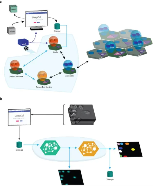
Figure 1: Cloud computing enables large-scale cellular image analysis with deep learning. (a) The software architecture of DeepCell 2.0. Blue lines signify flow of data while black lines signify flow of compute resources. Users begin by starting the kiosk container and specifying the parameters (user credentials, GPU type, etc.) of the cloud deployment. These parameters are used by Kubernetes to construct the cloud deployment and to assign pods (collections of containers) to their appropriate node. Some nodes can host multiple pods if appropriate. Trained models are stored in a cloud bucket and are available for inference. Uploaded data are placed in a cloud bucket, triggering the creation of an entry into a Redis queue. A data consumer communicates with the database and manages the analysis of a single data item. This communication includes submitting data to a deep learning model server and applying conventional computer-vision operations. Distinct data consumers can be written for specific workflows. Processed data are downloaded for further analysis. A custom autoscaling module monitors the Redis database to trigger 0-to-1 scaling of GPU nodes and TensorFlow serving. Once active, Kubernetes’ innate horizontal pod autoscaling capability monitors GPU utilization and dynamically adjusts the number of compute nodes and active pods to meet the data-analysis demand. (b) By hosting models on a centralized model server, DeepCell 2.0 allows for novel analysis workflows that require chaining multiple models. Here, we used a model that predicts images of cell nuclei from brightfield images and fed the output to a model that performs nuclear segmentation. This workflow removes the need for a fluorescent nuclear marker in live-cell imaging experiments, while the software infrastructure allows for scalable deployment on large imaging datasets.
9
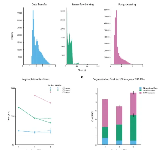
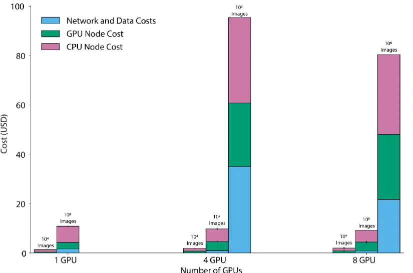
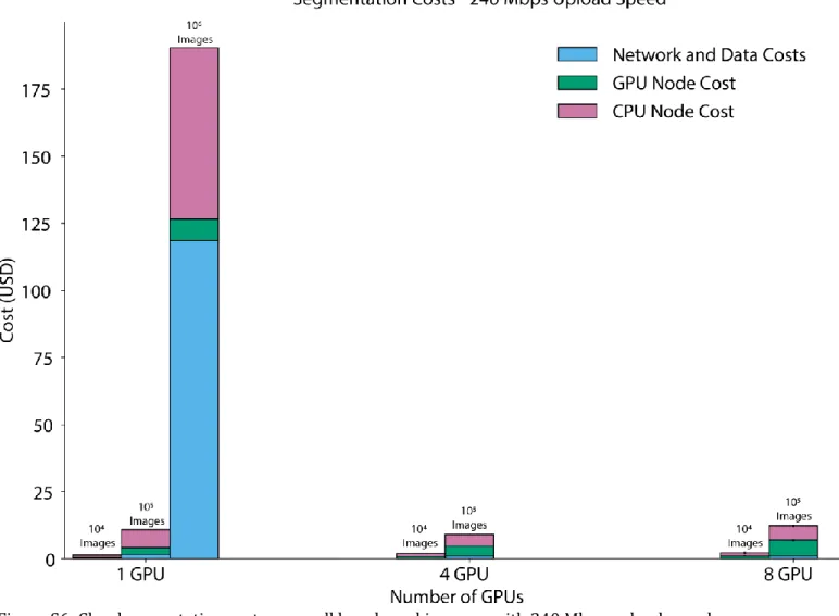
Figure 2: Benchmarking of DeepCell 2.0. (a) Contributions of data transfer, TensorFlow-serving latency, and post processing to the total runtime for individual images. These histograms denote the time required for each process during benchmarking for a 4GPU cluster with a 240 Mbps upload speed. For our tested model, latency from TensorFlow serving dominates the total processing time. Oscillations with a period of ~20 s arise from restarts. Despite considerable response time per-image, the high throughput of TensorFlow serving enables large-scale image analysis. (b) Total processing time for large imaging datasets. By scaling the cluster size dynamically to meet the data analysis demand, DeepCell 2.0 significantly reduces the time necessary to process large imaging datasets. Datasets consisting of 106 megapixel-scale images can be processed in several hours. An analysis of the tradeoff
between cluster size and upload speed appears in the Supplemental Information. Error bars in (b) and (c) represent the standard deviation. (c) Cost as a function of cluster size. While the cost of GPU nodes is considerable, it is mitigated by using pre-emptible instances for GPU inference. We see negligible differences in cost between small and large clusters to analyze large imaging datasets. Details of our benchmarking calculations appear in the Supplemental Information.
10
Supplemental Information
Cell lines and culturing. We used the mammalian cell lines NIH-3T3, HeLa-S3, HEK 293, and RAW 264.7 to collect training data for nuclear segmentation and the cell lines NIH-3T3 and RAW 264.7 to collect training data for augmented microscopy. All cell lines were acquired from ATCC. The cells have not been authenticated and were not tested for mycoplasma contamination.
Mammalian cells were cultured in Dulbecco’s modified Eagle’s medium (DMEM, Invitrogen or Caisson) supplemented with 2 mM L-glutamine (Gibco), 100 U/mL penicillin, 100 μg/mL streptomycin (Gibco or Caisson), and either 10% fetal bovine serum (Omega Scientific or Thermo Fisher; HeLa-S3 cells) or 10% calf serum (Colorado Serum Company; NIH-3T3 cells). Cells were incubated at 37 °C in a humidified 5% CO2 atmosphere.
When 70-80% confluent, cells were passaged and seeded onto fibronectin-coated, glass-bottom, 96-well plates (Thermo Fisher) at 10,000-20,000 cells/well. Seeded cells were incubated for 1-2 h to allow cells to adhere to the bottom of the well before imaging.
Collection of training data. For fluorescence nuclear imaging, mammalian cells were seeded onto fibronectin
(Sigma, 10 g/mL) -coated glass bottom 96-well plates (Nunc) and allowed to attach overnight. Medium was removed and replaced with imaging medium (FluoroBrite DMEM (Invitrogen) supplemented with 10 mM Hepes pH 7.4, 1% fetal bovine serum, 2 mM L-glutamine) at least 1 h before imaging. Cells without a genetically encoded nuclear marker were incubated with 50 ng/mL Hoechst 33342 (Sigma) before imaging. Cells were imaged with either a Nikon Ti-E or Nikon Ti2 fluorescence microscope with environmental control (37 °C, 5% CO2) and
controlled by Micro-Manager or Nikon Elements. Images were acquired with a 20x objective (40x for RAW 264.7 cells) and either an Andor Neo 5.5 CMOS camera with 2x2 binning or a Photometrics Prime 95B CMOS camera with 2x2 binning. All data were scaled so that pixels had the same physical dimension prior to training.
For our augmented microscopy training dataset, which consisted of brightfield and fluorescence nuclear images, cells were imaged on a Nikon Eclipse Ti-2 fluorescence microscope with environmental control (37 °C, 5% CO2) at
20x and 40x for NIH-3T3 and RAW264.7 cells, respectively. Nuclei were labeled with Hoescht 33342. Each dataset was generated by collecting a fluorescence image in the focal plane as well as a z-stack of phase images (0.25 µm slices, ±7.5 µm from focal center). Images were collected on a Photometrics Prime 95B CMOS camera with no binning.
Autoscaling policy. We developed novel scaling policies for the redis consumer and TensorFlow (TF)-serving pods. The TF-serving pod processes images with deep learning models, while the data-consumer pod feeds data into TF serving. The scaling of these two pods is linked, as the data-consumer pods drive utilization of the TF-serving pods. We observed that while data-consumer pods can bottleneck inference speed, having too many data-consumer pods present at once results in an effective “denial of service” attack on the TF-serving pods.
To optimally scale both pods, we use autoscaling policies that are based on GPU utilization and work demand. Because of the distributed nature of our task, we use horizontal pod autoscaling (more nodes) to scale our cluster as opposed to vertical pod autoscaling (bigger nodes). Our metrics, available through Prometheus, provide the information necessary for scaling. Horizontal pod autoscaling in Kubernetes works by defining a metric and a target for a given pod. If the metric, measured over a given time period, is larger than the target, then the pod is scaled up; if it is smaller, then it is scaled down. The target number of pods is given by 𝑁𝑝𝑜𝑑𝑠= 𝑁𝑐𝑢𝑟𝑟𝑒𝑛𝑡 𝑝𝑜𝑑𝑠
𝑚𝑒𝑡𝑟𝑖𝑐 𝑡𝑎𝑟𝑔𝑒𝑡. Typical metrics are based on resource utilization: if utilization is too high (metric > target), then the pod needs to be larger. If it is too low (metric < target), then the pod needs to smaller. For the TF-serving pod, we set our metric to be GPU utilization, which ranges from 0% to 100%, and the target to be 70%. For the data-consumer pod, we set our metric to be 𝑚𝑒𝑡𝑟𝑖𝑐 = { 0 𝑖𝑓 𝑇𝐹 𝑠𝑒𝑟𝑣𝑖𝑛𝑔 𝑝𝑜𝑑𝑠 = 0 𝑚𝑖𝑛 (100−𝐺𝑃𝑈 𝑢𝑡𝑖𝑙𝑖𝑧𝑎𝑡𝑖𝑜𝑛 100 , #𝑝𝑟𝑒𝑑𝑖𝑐𝑡 𝑘𝑒𝑦𝑠 #𝑟𝑒𝑑𝑖𝑠 𝑐𝑜𝑛𝑠𝑢𝑚𝑒𝑟 𝑝𝑜𝑑𝑠) 𝑖𝑓 #𝑟𝑒𝑑𝑖𝑠 𝑐𝑜𝑛𝑠𝑢𝑚𝑒𝑟 𝑝𝑜𝑑𝑠 #𝑇𝐹 𝑠𝑒𝑟𝑣𝑖𝑛𝑔 𝑝𝑜𝑑𝑠 < 150 𝑒𝑙𝑠𝑒 0.135 .
11
The target for this metric is set to be 0.15 for several reasons. First, the goal of this scaling policy is to create enough data consumers to efficiently drive the TF-serving pod; tying scaling criteria to the GPU utilization effectively achieves this goal. Second, because we have consumers of different types, care must be taken to ensure that scaling is also sensitive to the amount of work, in order to ensure that new processing tasks are assigned consumers. The work metric measures how much work has built up in the queue; if the amount of work to do is high, then the scaling policy overrides the GPU utilization-based metric to scale up the pod.
Model architecture and training. The code for every model is available at https://www.github.com/deepcell-tf
under the deepcell.model_zoo module. We used feature-nets extensively in this work for benchmarking. Feature-nets are a deep learning model architecture for general-purpose image segmentation. We previously used various feature-nets for nuclear segmentation in 2D cell culture images6, 3D confocal images of brain tissue35, and 2D
multiplexed ion beam imaging datasets5. This architecture has also been applied to single-cell segmentation of
bacteria6 and yeast36. The key feature of this architecture is its ability to treat the deep learning model’s receptive
field—the length scale over which it pays attention—as a tunable variable. Our prior work revealed that deep learning models work best when the receptive field size is matched to the feature size of a given dataset37. This
intuition has been valid for both feature-nets and object detection-based approaches like Mask-RCNN (data not shown). Given the diversity in cellular morphologies across the domains of life, we believe that feature-nets are a good starting point for cell biologists seeking to apply deep learning to new datasets.
We trained three models for this work. The first model was a feature-net for 2D image segmentation using a deep watershed approach with a 41-pixel receptive field for benchmarking. This model was trained in a fully convolutional fashion using stochastic gradient descent with momentum of 0.9, a learning rate of 0.01, weight decay of 10-6, and an L2 regularization strength of 10-5 for 5 epochs on a NVIDIA V100 graphics card. A dataset
consisting of ~300,000 cell nuclei annotations was used for training.
For nuclear segmentation of brightfield images, we trained two models. The first of these models transforms brightfield images into nuclear images. We used a modified 3D feature-net with a 41-pixel receptive field where dilated max pooling layers are replaced with 2D convolutional layers with kernel size 2 and an equivalent dilation rate. This model was trained in a fully convolutional fashion for using stochastic gradient descent with momentum with a learning rate of 0.01, momentum of 0.9, weight decay of 10-6, and an L2 regularization strength of 10-5 for 5
epochs on a NVIDIA V100 graphics card. A dataset consisting of matched brightfield image stacks and fluorescent nuclear images was used for training.
The second model for brightfield images was a modified RetinaMask38 model for nuclear segmentation.
RetinaMask generates instance masks in a fashion similar to Mask-RCNN but uses single-shot detection like RetinaNet33 rather than feature proposals39 to identify objects. We used a ResNet50 backbone and the P2, P3, and
P4 feature pyramid layers for object detection. We also used custom anchor sizes of 8, 16, and 32 pixels for each of these layers. This model was trained using the Adam optimization algorithm40 with a learning rate of 10-5, clipnorm
of 0.001, batch size of 4, and L2 regularization strength of 10-5 for 16 epochs on a NVIDIA V100 graphics card. A
dataset consisting of ~300,000 cell nuclei annotations was used for training.
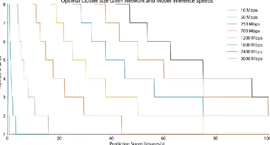
Relationship between data transfer rates, inference speeds, and cluster size. Data transfer poses a fundamental limit to how quickly data can be analyzed. A cluster that is operating efficiently processes data at the same rate that the data enter. Given a data transfer speed d and a single model with an inference speed of s, this leads to the equation
𝑑 = 𝑁𝐺𝑃𝑈𝑠,
where NGPU, the number of GPUs in the cluster, is effectively the cluster size. A plot of this optimal cluster size as a
12
Figure S1: Optimal cluster size as a function of model inference speed and data upload speeds.
Benchmarking details. For benchmarking, data were gathered using the kiosk-benchmarking repo
(github.com/vanvalenlab/kiosk-benchmarking). All runs of 10,000 or 100,000 images were done in triplicate. Runs of 1,000,000 images were run a single time. All data in Figure 2a of the main text were derived from timestamps taken from redis-consumer pods within the cluster. Data Transfer Times from Figure 2a of the main text were calculated by doubling the sum of the time it took a redis-consumer pod to download a raw image from the storage bucket and then upload the resulting image to the storage bucket. This calculation may mildly underestimate the total time a given image spends in transit in the cluster, since the image must go through several transfer steps:
1) Upload to storage bucket as part of a zip file.
2) Download of zip file from storage bucket by zip-consumer pod.
3) Upload of individual raw image to storage bucket from zip-consumer pod. 4) Download of individual raw image from storage bucket by redis-consumer pod. 5) Upload of individual predicted image to storage bucket from redis-consumer pod. 6) Download of individual predicted image from storage bucket to zip-consumer pod. 7) Upload of zipped batch of predicted images to storage bucket from zip-consumer pod. 8) Download of zipped batch of predicted images from storage bucket by client.
Our methodology accounts reasonably for steps 3-6, but not steps 1-2 and 7-8. TF Serving Response Times in Figure 2a of the main text were the amount of time redis-consumer pods had to wait for a response from TF-serving pods. Postprocessing Times in Figure 2a of the main text were the amount of time that a redis-consumer pod was occupied carrying out post-processing computations on the results received from TF-serving pods. In Figure 2b of the main text, Number of GPUs refers to the maximum number of GPUs available to a cluster, whether the cluster ever scaled up to the point where that number of GPUs was being utilized simultaneously. NVIDIA Tesla-V100 GPUs were used in all benchmarking runs. In Figure 2c of the main text, costs were computed following methodology documented in the vanvalenlab/kiosk-benchmarking repository.
13
Benchmarking data. All data from our benchmarking are shown below. Each run was performed in triplicate, except for the 1M image runs, which were performed once.
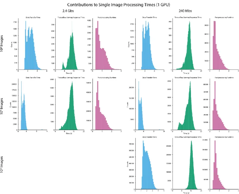
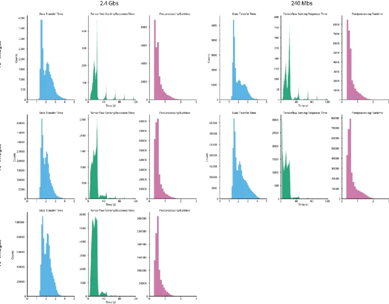
Figure S2: Contributions of data transfer time, Tensorflow serving response time, and post processing time to the time required to process a single image. Data for clusters with 1 GPU are shown.
14
Figure S3: Contributions of data transfer time, Tensorflow serving response time, and post processing time to the time required to process a single image. Data for clusters with a maximum of 4 GPUs are shown.
15
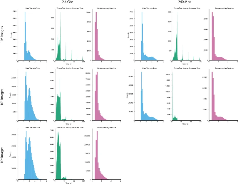
Figure S4: Contributions of data transfer time, Tensorflow serving response time, and post processing time to the time required to process a single image. Data for clusters with a maximum of 8 GPUs are shown.
16
17