Distributional Changes in the Gender Wage Gap

RUHR

ECONOMIC PAPERS

Distributional Changes

in the Gender Wage Gap

Imprint

Ruhr Economic Papers

Published by

Ruhr-Universität Bochum (RUB), Department of Economics Universitätsstr. 150, 44801 Bochum, Germany

Technische Universität Dortmund, Department of Economic and Social Sciences Vogelpothsweg 87, 44227 Dortmund, Germany

Universität Duisburg-Essen, Department of Economics Universitätsstr. 12, 45117 Essen, Germany

Rheinisch-Westfälisches Institut für Wirtschaftsforschung (RWI) Hohenzollernstr. 1-3, 45128 Essen, Germany

Editors

Prof. Dr. Thomas K. Bauer

RUB, Department of Economics, Empirical Economics Phone: +49 (0) 234/3 22 83 41, e-mail: thomas.bauer@rub.de Prof. Dr. Wolfgang Leininger

Technische Universität Dortmund, Department of Economic and Social Sciences Economics – Microeconomics

Phone: +49 (0) 231/7 55-3297, email: W.Leininger@wiso.uni-dortmund.de Prof. Dr. Volker Clausen

University of Duisburg-Essen, Department of Economics International Economics

Phone: +49 (0) 201/1 83 -3655, e-mail: vclausen@vwl.uni-due.de Prof. Dr. Christoph M. Schmidt

RWI, Phone: +49 (0) 201/81 49 -227, e-mail: christoph.schmidt@rwi-essen.de

Editorial Offi ce

Joachim Schmidt

RWI, Phone: +49 (0) 201/81 49 -292, e-mail: joachim.schmidt@rwi-essen.de

Ruhr Economic Papers #220

Responsible Editor: Christoph M. Schmidt

All rights reserved. Bochum, Dortmund, Duisburg, Essen, Germany, 2010 ISSN 1864-4872 (online) – ISBN 978-3-86788-252-1

Ruhr Economic Papers #220

Distributional Changes

in the Gender Wage Gap

Bibliografi sche Informationen

der Deutschen Nationalbibliothek

Die Deutsche Bibliothek verzeichnet diese Publikation in der deutschen National-bibliografi e; detaillierte National-bibliografi sche Daten sind im Internet über:

http://dnb.d-nb.de abrufb ar.

Sonja Kassenböhmer and Mathias Sinning1

Distributional Changes in the Gender

Wage Gap

Abstract

This paper analyzes changes in wage diff erentials between white men and white women over the period 1993–2006 across the entire wage distribution using Panel Study of Income Dynamics (PSID) data. We decompose distributional changes in the gender wage gap to assess the contribution of observed characteristics measuring individual productivity. We fi nd that the gender wage gap narrowed by more than 13 percent at the lowest decile and by less than 4 percent at the highest decile. The decomposition results indicate that changes in the gender wage gap are mainly attributable to changes in educational attainment at the top of the wage distribution, while a sizeable part of the changes is due to work history changes at the bottom. Our fi ndings suggest that the educational success of women could reduce the gender wage gap at the bottom of the distribution both before and during the 1990s but did not trigger a strong decline at the top of the distribution until today.

JEL Classifi cation: C21, J16, J31

Keywords: Gender wage gap; decomposition analysis; unconditional quantile regression November 2010

1 Sonja Kassenböhmer, RWI; Mathias Sinning, Australian National University, RWI and IZA. – Deborah Cobb-Clark, Tue Gørgens, John Haisken-DeNew, Christoph Rothe and participants of the 2010 meeting of the European Society for Population Economics (ESPE) and the joint 2010 meeting of the Society of Labor Economics (SOLE) and the European Association of Labour Economists (EALE) provided valuable comments and suggestions on earlier drafts of this paper. – All correspondence to Mathias Sinning, Research School of Economics (RSE), HW Arndt Building

1

Introduction

After decades of relative constancy, the gender wage gap in the U.S. has fallen steadily since the late 1970s. The decline in the gender wage gap during the 1980s was typ-ically explained by increases in educational attainment among younger women and increases in labor market experience among older women (Wellington, 1993; O’Neill and Polachek, 1993; Blau and Kahn, 1997; Pissarides et al., 2005). In contrast, re-searchers were often unable to attribute the slower wage convergence during the 1990s to factors that were observed in the data (O’Neill, 2003; Blau and Kahn, 2006).1

While the economic literature has focused predominantly on the gender wage gap at the mean, several recent studies have examined wage disparities across the entire wage distribution (García et al., 2001; Albrecht et al., 2003; Blau and Kahn, 2006; Gupta et al., 2006; Arulampalam et al., 2007; Antonczyk et al., 2010).2_{Interestingly,} very little is known about the factors that are responsible for changes in the gender wage gap across the wage distribution although the factors that explain the gender wage gap are not necessarily responsible for changes in this gap and the factors that are relevant at the bottom of the wage distribution may be irrelevant at the top.

Empirical studies have typically employed decomposition methods to investigate the extent to which wage determinants affect the gender wage gap. Departing from the standard decomposition method of Blinder (1973) and Oaxaca (1973), a number of decomposition methods for wage distributions have been proposed (such as Juhn et al., 1993; DiNardo et al., 1996; Gosling et al., 2000; Melly, 2005; Machado and Mata, 2005; Rothe, 2010a). However, the decomposition results of distributional 1_{As a result, recent studies have started to investigate the relevance of typically} unobserved non-cognitive factors, such as behavioral or personality traits (Bowles et al., 2001; Judge et al., 2001; Manning and Swaffield, 2005; Kuhn and Weinberger, 2005; Heckman et al., 2006; Waddell, 2006; Fortin, 2008; Borghans et al., 2008). The estimated relationship between non-cognitive factors and outcomes varies consider-ably across studies.

2_{On balance, these studies have produced rather mixed results. Arulampalam et} al. (2007), for example, find substantial heterogeneity in the gender wage gap across wage distributions of several European countries.

measures obtained by these methods are not comparable to those of the standard Blinder-Oaxaca decomposition of the mean wage differential. In fact, none of these methods produces consistent results when changes in the gender wage gap over time are being studied, while the results of a Blinder-Oaxaca decomposition of changes in the gender wage gap between two points in time are consistent with those of a decomposition of gender differences in wage growth over this period (given the use of a common reference vector as defined by Oaxaca and Ransom, 1994).

This paper contributes to the economic literature by investigating changes in the gender wage gap across the entire distribution. We apply a newly-developed Blinder-Oaxaca type decomposition for unconditional quantile regression models (Firpo et al., 2007a,b, 2009) to decompose wage differentials across the wage distribution. This method allows us to decompose the wage differential for any quantile in the same way means are decomposed using the standard Blinder-Oaxaca decomposition. The approach also permits a partition of the overall components of the decomposition equation into the contribution of individual characteristics or groups of character-istics. In our empirical analysis, we pay particular attention to the relevance of measures of individual productivity, such as education and labor market experience. We utilize data from the 1994 and 2007 waves of the Panel Study of Income Dy-namics (PSID), which is the only nationally representative data source in the U.S. that contains information on actual labor market experience and other relevant work history information. Several studies have shown that the work history is a very im-portant factor in explaining changes in the gender wage gap (O’Neill and Polachek, 1993; Blau and Kahn, 2006).

To investigate the contribution of individual (groups of) characteristics, we de-compose the gender wage gap in 1993 and 2006. Our approach is similar to that of Wellington (1993) who decomposes changes in the gender wage gap at the mean. We further perform separate decompositions of changes in wage levels over the pe-riod 1993-2006 for male and female workers. Finally, we present the decomposition results of changes in the gender wage gap which are identical to the decomposition

results of gender differences in wage growth. We are particularly interested in ad-dressing the following questions: To what extent did the gender wage gap decline over the period 1993-2006? Did the gender wage gap decline because observed char-acteristics changed in favor of women or because the returns to these charchar-acteristics changed over time? How do the results vary across the wage distribution? These are important questions given the slowing convergence in the gender wage gap and the evidence for variations in the gap across the wage distribution (Blau and Kahn, 2006).

Our findings indicate that the gender wage gap narrowed by more than 13 percent at the lowest decile and by less than 4 percent at the highest decile of the wage distribution between 1993 and 2006. On average, the gap decreased by about 7 percent. The results of the decomposition analysis indicate that the decline in the gender wage gap at the upper tail of the distribution may be attributed entirely to changes in educational attainment in favor of female workers. At the same time, a sizeable part of the decline at the lower tail of the distribution is due to work history changes. These findings point to substantial heterogeneity with regard to the decline in the gender wage gap across the distribution and the relevance of the factors that are responsible for this decline. Due to the relatively small part of changes in the gap at the bottom of the distribution that is explained by education, it seems likely that the educational success of women did contribute to a reduction in the gender wage gap at the lower end of the distribution since the 1970s. Our findings also suggest that this success could not trigger a strong decline at the top of the distribution until today.

The remainder of the paper is organized as follows. Section 2 includes a descrip-tion of the data and provides a descriptive analysis of wage distribudescrip-tions and wage determinants. The empirical strategy is explained in Section 3. Section 4 discusses the empirical findings of the decomposition analysis. Section 5 concludes.

2

Data and Descriptive Analysis

2.1

Data

Our empirical analysis employs data from the Panel Study of Income Dynamics (PSID), a nationally representative longitudinal study of almost 9,000 U.S. families which started in 1968. Our analysis focuses on the years 1994 and 2007 because wages were surveyed consistently over this period. These two survey years allow us to analyse average hourly earnings of male and female workers in 1993 and 2006.3_The inflation calculator of the Bureau of Labor Statistics is used to calculate average real earnings in 1993 dollars. We focus on the PSID Core sample and employ the sampling weights provided in the PSID files.4_{We restrict our sample to white male and female} full-time employed workers who are either head or wife of their household. We define full-time employed workers as persons who are not self-employed and who reported to work at least 1,500 hours during the year. However, we also use an extended sample including persons who work less than 1,500 hours to address selection issues. We further restrict the sample to individuals aged 25 to 62 years to avoid selection problems with young adults who are heads or wives of their own households and to exclude older persons who retire early. Moreover, members of the armed forces are removed from our sample.

The set of explanatory variables used in our analysis can be divided into four categories: 1) educational attainment, 2) work history, 3) union membership and 4) region of the country. We use indicator variables of the highest level of formal ed-ucation as explanatory variables. Specifically, the PSID provides information about the following levels of formal education: 1) 8th grade and below, 2) 9th to 11th grade, 3_{Following Blau and Kahn (2006), we will refer to the earnings dates (1993 and} 2006) throughout the paper but consider explanatory variables that were measured at the survey date (1994 and 2007).

4_{The PSID Core sample is a combination of the Survey Research Center (SRC)} sample and the Survey of Economic Opportunity (SEO) sample. Gouskova et al. (2008) provide a more detailed description of the PSID sample design and composi-tion.

3) 12th grade (high school), 4) 12 grades plus nonacademic training, 5) college but no degree, 6) college BA but no advanced degree, 7) college and advanced or pro-fessional degree. We further utilize the detailed information on work experience and tenure to generate a set of work history variables. Specifically, we consider quadratic functions of the number of years of work experience, the number of years worked full-time since age 18 and tenure with the current employer.5_{The number of years} of full-time employment is included to account for the possibility that part-time em-ployment has no significant effect on wage growth. In addition, we control for the total number of years with the current employer, which typically explains a sizeable part of the gender wage gap (see, e.g., Fortin, 2008). We further include an indicator variable for union membership into our model to control for the possibility that vari-ations in union membership have affected changes in the gender wage gap. Finally, regional division indicators were included to control for regional wage differentials and regional variations in wage dynamics.6

Since women may be disproportionately concentrated in relatively low-paying jobs, we follow Wellington (1993) and do not include occupation indicators in our model. Instead, our analysis focuses on the contribution of productivity differences to the wage differential. As a result, the part of the wage differential attributable to occupational segregation is interpreted as contributing to the “unexplained” part of the gap which may be due to omitted variables or discrimination.

2.2

Distributional Changes

Table 1 presents the wages of male and female workers in 1993 and 2006 across the respective wage distribution. The numbers reveal that the 6.8 percent increase in 5_{Data on work experience of persons surveyed in 1993 was not brought forward} to the 1994 PSID file. For that reason, work experience information from 1993 data was used for heads and wives who were surveyed in both years.

6_{Specifically, we employ the nine regional divisions used by the U.S. Census} Bu-reau (New England, Mid-Atlantic, East North Central, West North Central, South Atlantic, East South Central, West North Central, Mountain, Pacific).

real wages for male workers between 1993 and 2006 is mainly the result of the strong wage increase of 14.3 percent at the highest decile of the male wage distribution. Real wages of male workers have even declined at the median and the bottom of the distribution. Over the same period, average real wages of female workers have increased by 8.7 percent. In contrast to the changes in wage distributions of male workers, wages of female workers have increased substantially across the entire distri-bution. These increases were particularly strong at the 30th and the 90th percentile of the female wage distribution.

As a result of these changes, the female-male wage ratio presented in the last two columns of Table 1 increased considerably at the lower tail of the distribution, while the increase at the upper tail of the distribution was rather moderate. Specifically, while the wage ratio surged from 65.1 percent in 1993 to 72.7 percent in 2006 at the lowest decile, it only increased from 72.6 percent in 1993 to 72.9 percent in 2006 at the highest decile. On average, the wage ratio increased from 71.3 percent in 1993 to 72.6 percent in 2006. These numbers suggest that average changes in the gender wage gap between 1993 and 2006 were rather moderate, while the gap narrowed considerably at the bottom of the distribution, highlighting the importance of a distributional analysis of the changes in the gender wage gap.7

2.3

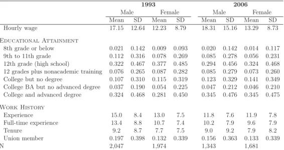
Comparison of Explanatory Variables by Gender

The means and standard deviations of male and female workers in 1993 and 2006 are presented in Table 2. The numbers provide evidence for a strong increase in the 7_{Our wage patterns are in line with those of Blau and Kahn (2004) who show that} their findings based on PSID data are consistent with Current Population Survey (CPS) data. Differences between wage patterns of Blau and Kahn (2004, 2006) and our study are due to both the choice of different survey years and different sample restrictions. In particular, when comparing different age restrictions, we find that we observe a much larger gap at the bottom of the wage distribution than Blau and Kahn (2004, 2006) because we restrict our sample to 25-62 rather than 18-65 year old workers. Since our empirical analysis focuses on temporal changes rather than levels, a detailed comparison of wage levels with similar studies is beyond the scope of the paper.

share of female workers with an advanced university degree from 28.1 percent in 1993 to 34.5 percent in 2006. While female workers were less likely than male workers to hold an advanced university degree in 1993, the share of female workers with such a degree was as high as the share of male workers in 2006. As a consequence, the overall share of female workers who went to college (with or without having a degree) in 2006 was higher than the respective share of male workers.

The numbers of the work history variables indicate that a substantial decline in work experience has taken place for both male and female workers. While the average number of years of work experience dropped from 15.0 in 1993 to 11.8 in 2006 among male workers, the average experience of female workers decreased from 13.0 years in 1993 to 11.9 years in 2006. Correspondingly, the number of years of full-time experience declined by 3.2 years among male workers and by 1.1 years among female workers. While the labor market experience of workers declined over time, the average number of years with the current employer has remained relatively constant. Specifically, job tenure decreased from 9.2 years in 1993 to 9.0 years in 2006 among male workers and increased from 7.7 years in 1993 to 7.9 years in 2006 among female workers. Due to the substantial decline in the average labor market experience among male workers, the overall changes in work history characteristics could be in favor of female workers. Moreover, the numbers show a convergence in union membership between male and female workers, although the differences observed in 2006 remain sizeable. Specifically, while the share of union members in the group of male workers dropped from 19.7 percent in 1993 to 15.6 percent in 2006, union membership increased moderately from 13.2 percent in 1993 to 13.3 percent in 2007 among female workers.

In sum, these numbers provide evidence for considerable changes in character-istics that describe the productivity of male and female workers. Although most variables seem to have changed in favor of female workers, we do not know whether the observed decline in the gender wage gap (Table 1) may be attributed to changes in characteristics or whether changes in returns to the characteristics were

respon-sible for the narrowing of the gender wage gap. The following sub-section presents the estimates of the returns to the characteristics.

2.4

Returns to Productivity Characteristics by Gender

Table 3 includes the OLS estimates of a regression of log wages on the set of regressors discussed above. Specifically, our model includes indicator variables for the highest level of formal education (we use workers with a formal education of grade 8 or below as a reference group), quadratic functions of work history characteristics (i.e. the number of years of actual work experience, the number of years of full-time work experience and tenure) and an indicator variable for union membership. In addition, our model includes state fixed-effects. Tables A1-A4 of the Appendix include the corresponding estimates of the unconditional quantile regression model.

The estimates in Table 3 show highly significant effects of educational attainment on wages of both male and female workers. The returns to education differ somewhat between male and female workers and have slightly increased over time. Our findings further suggest that job tenure is an important wage determinant, while the actual labor market experience of both male and female workers seems to be less relevant. While union membership increased the wage rate of male workers in 1993, the corre-sponding effect is not significant in 2006. In contrast, union membership effects are not significant at conventional levels for female workers in both years. Overall, these findings point to some heterogeneity in the effects of productivity characteristics on wages of male and female workers in both years.

3

Empirical Strategy

3.1

Decomposition of the Mean Wage Differential

Our empirical analysis departs from the standard Blinder-Oaxaca decomposition. Specifically, we consider the wage differential between two groupsd = (0,1). We

observe the (log) wageYidand a set of characteristicsXidfor each workeriin groupd and assume that the conditional expectation ofYdgivenXdis linear so that

E[Yid|Xid] = Xidβd, d= 0,1. (1)

To isolate the part of the raw wage differential (R) between the two groups at-tributable to differences in observed characteristics or “endowments” from the part due to differences in coefficients, the decomposition proposed by Blinder (1973) and Oaxaca (1973) and generalized by Oaxaca and Ransom (1994) can be written as follows: R = E(Y₁)−E(Y₀) =E(X₁)β₁−E(X₀)β₀ (2) = [E(X₁)−E(X₀)]β∗ endowments +E(X₁)(β₁−β∗) +E(X₀)(β∗−β₀) coefficients ,

where the reference vectorβ∗is given by the linear combination

β∗ = Ωβ₁+ (I−Ω)β₀.

The first term on the right-hand side of equation (2) is interpreted as the part of the raw gap that may be explained by different observed characteristics, while the two remaining terms are attributable to different coefficients between the two groups.

3.2

Decomposition of Wage Distributions

The Blinder-Oaxaca decomposition relies on an important property: Due to the law of iterated expectations, a linear model for the conditional expectation implies that

EX[E(Yd|Xd)] =E(Yd) =E(Xd)βd.Parametric extensions of the Blinder-Oaxaca decomposition to entire wage distributions have typically employed conditional quan-tile regressions (Koenker and Basset, 1978) to decompose the wage gap at a given quantile ofY. However, the interpretation of these methods is complicated by the fact that conditional quantiles do not average up to their unconditional

counter-parts. Against this background, Firpo et al. (2007b, 2009) propose an uncondi-tional quantile regression based on a recentered influence function (RIF). Specifi-cally, they consider the influence function (IF) for a quantileqτ which is equal to

(τ−₁{Y ≤qτ})/fY(qτ),wherefY(·)is the marginal density function ofY. Given the recentered influence function RIF(Y;qτ) =qτ+IF(Y;qτ), they define the uncon-ditional quantile regression model as the conuncon-ditional expectation of the RIF(Y;qτ) givenX: E[RIF(Y;qτ)|X].Firpo et al. (2007a) show that a Blinder-Oaxaca type decomposition based on RIF-regression estimates can be approximated for any dis-tributional statistic, including quantiles. In particular, under the strong assumption that E[RIF(Y;qτ)|X]is linear in X, the (predicted) wage differential at theτth quantile,R(τ), may be decomposed as follows:

R(τ) = E(X₁)β₁(τ)−E(X₀)β₀(τ) (3) = [E(X₁)−E(X₀)]β∗(τ) endowments +E(X₁)(β₁(τ)−β∗(τ)) +E(X₀)(β∗(τ)−β₀(τ)) coefficients , with β(τ)∗ = Ω(τ)β₁(τ) + (I−Ω(τ))β₀(τ),

whereβ₁(τ) and β₀(τ)are the parameters of the unconditional quantile regression model at theτth quantile. Due to the linearity assumption, the proposed extension of the Blinder-Oaxaca decomposition based on unconditional quantile regression es-timates is straightforward.8_{For that reason, we may limit our following discussion} to the standard Blinder-Oaxaca decomposition of mean wage differentials.

8_{Note that the assumption of a linear RIF-regression function used to define the} decomposition is not unproblematic. As argued in Rothe (2010b), it implies that the respective feature of the outcome distribution depends on the marginal distribution of the covariates only through their mean. We consider the RIF-regression estimates as weights that allow us to perform a unique decomposition analysis.

3.3

Choice of the Counterfactual Parameter Vector

Considerable work in the literature has been on the particular choice of the weight-ing matrixΩand the resulting reference vector. While the decomposition equations originally proposed by Blinder (1973) and Oaxaca (1973) were based on the assump-tion that differences in coefficients may be attributed exclusively to the disadvantage of the group with the lower outcome (i.e. β∗= β₁) or the advantage of the group with the higher outcome (i.e. β∗=β₀), economists have argued that an undervalu-ation of one group implies an overvaluundervalu-ation of the other. Reimers (1983) therefore proposes to calculate the reference vector by using the average coefficients over both groups, i.e.ΩR_{= 0.5I. Cotton (1988) chooses the weighting matrixΩ}C_{=sI, where}

sdenotes the sample share of the group with the higher outcome. Finally, Neumark (1988) proposes the estimation of a pooled model over both groups, i.e.

Yi = αN+Xiβ N_+εN

i i= 1, ..., N. (4)

The strategy proposed by Neumark (1988) has become a widely adopted alternative to the decomposition equation originally proposed by Blinder (1973) and Oaxaca (1973). However, recent studies have shown that this strategy systematically over-states the explained part of an overall gap because the estimated parameter vector

βN _{suffers from omitted variable bias caused by the missing group-specific} inter-cept (Fortin, 2008; Jann, 2008; Elder et al., 2010).9 _{They propose to estimate the} reference vector through a pooled linear regression model of the form

Yi = αP+βdPdi+Xiβ P_+εP

i i= 1, ..., N. (5)

In the following, we will employ an extension of this strategy that allows us to decompose changes in wage differentials over time.

9_{Elder et al. (2010) note that Neumark (1988) starts from the assumption that} the set of observable characteristics is sufficiently rich to remove all productivity differences between the two groups of interest. It is unlikely that this assumption holds for many other applications.

3.4

Estimation of Changes in Wage Differentials

In our empirical analysis, we decompose wages of male and female workers in 1993 and 2006, i.e. we consider four sub-samples rather than two. Specifically, we define

di1= 1if individualiis a male worker anddi1= 0if individualiis a female worker. Similarly, we definedi2= 1if individualiis observed in 2006 anddi2= 0otherwise. A natural choice of the reference vector for this extension is the coefficient vectorβX of the following pooled regression model:

Yi = α+βd1di1+βd2di2+βd12di1di2+XiβX+εi i= 1, ..., N, (6) whereN is the total number of observations of the pooled model including the four sub-samples (i.e. male and female workers in 1993 and 2006). We may estimate the parameter vectorβ∗byβX to decompose the gender wage gap at two points in time. Specifically, we may decompose the wage differential between male (m) and female (f) workers at timet= (1993,2006)as follows:

(Ymt−Yf t) = Δt=Et+Ct, (7)

whereEt = (Xmt−Xf t)βXandCt = Xmt(βX−βmt) +Xf t(βf t−βX).Similarly, we may decompose the wage growth between 1993 and 2006 within one of the two groupsg= (m, f):

(Yg2006−Yg1993) = Δg=Eg+Cg, (8) withEg= (Xg2006−Xg1993)βX andCg=X

g2006(βX−βg2006) +Xg1993(βg1993−βX). Given equations (7) and (8), we can derive the following decomposition of changes in the gender wage gap over time, which is equivalent to a decomposition of gender

differences in wage growth, i.e. Δ2006−Δ1993 = (E2006−E1993) + (C2006−C1993) (9) = Δm−Δf = (Em−Ef) + (Cm−Cf), with(E₂₀₀₆−E₁₉₉₃) = (Em−Ef)and(C2006−C1993) = (Cm−Cf).

3.5

Detailed Decomposition and Grouping

To understand the source of the gender wage gap, we decompose the wage differ-ential into components describing the contribution of individual characteristics or groups of characteristics. Such a detailed decomposition of the wage differential requires the consideration of several methodological issues. First, it is well known that the arbitrary scaling of continuous variables may affect the components of the gap attributable to different coefficients (Jones, 1983; Jones and Kelley, 1984; Cain, 1986). For that reason, we consider the part of the gap due to different coefficients as unexplained without performing a detailed decomposition of this component.

Second, we group most of the variables included in our model to facilitate an interpretation of the results. Specifically, we consider four groups of characteristics: 1) “Education” (i.e. indicator variables of the highest level of formal education), 2) “Work History” (i.e. variables describing the individual work history), 3) “Union membership” (measured by an indicator variable), and 4) “Region” (i.e. indicator variables of the regional division of residence). Jann (2008) provides a detailed de-scription of the calculation of standard errors for all components of the decomposition equation.

Third, the detailed decomposition for categorical regressors depends on the choice of the reference category that is omitted from the regression model due to collinearity (Oaxaca and Ransom, 1999; Horrace and Oaxaca, 2001; Gardeazabal and Ugidos, 2004; Yun, 2005). Gardeazabal and Ugidos (2004) and Yun (2005) propose

normal-izations of the coefficients of categorical variables to avoid having omitted reference groups. However, these normalizations may complicate the interpretation of the de-composition results, which still depend on the choice of reference groups (Gelbach, 2002; Fortin et al., 2010). In our empirical analysis, we consider the lowest level of education (8th grade or below), the group of non-union workers and the region Pacific (Alaska, Washington, Oregon, California, Hawaii) as reference groups. Due to the grouping of variables, the choice of alternative reference groups does not affect our results qualitatively.

3.6

Correction for Selection Bias

As described above, we may extend the results derived for the conventional Blinder-Oaxaca decomposition to any quantile by performing a Blinder-Blinder-Oaxaca type decom-position of unconditional quantile regression estimates. In addition, we will also employ an extension of the standard decomposition to Heckman selection models (see Neuman and Oaxaca, 2004) to correct for selectivity bias at the mean. The marital status and the number of children will be used as exclusion restrictions to model participation in full-time employment. The following sub-section presents the decomposition results for the OLS model, the Heckman selection model and the unconditional quantile regression model. While the results of the conventional Blinder-Oaxaca decomposition and the unconditional quantile regression decompo-sition is presented according to equations (7), (8) and (9), the decompodecompo-sition of the Heckman selection model is limited to equations (7) and (8).10

4

Results

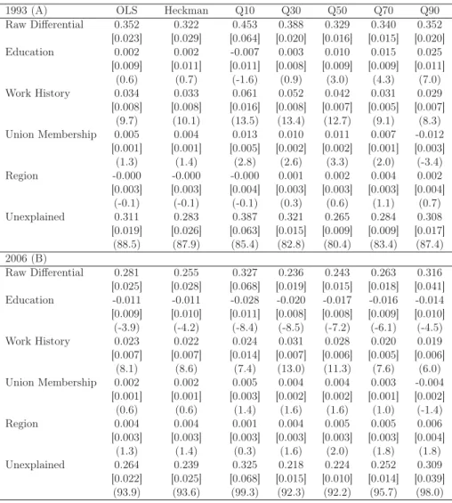
Table 4 includes the decomposition results for the wage differential between male and female workers in 1993 (A) and 2006 (B). The estimates in the upper panel 10_{Since the selection bias correction term is a non-linear function, we cannot use} estimates of the selection model to decompose changes in the gender wage gap.

(Panel A) of Table 4 show an average wage gap of 0.352 log points (42.2 percent).11 That gap dropped to 0.281 log points (32.4 percent) in 2006 (Panel B).

Comparing the decomposition results of the OLS model to those of the Heckman selection model suggests that selection into full-time employment does not affect the decomposition results substantially. This finding is in line with the estimates of the selection model presented in Tables A5 and A6 of the appendix, which indicate that selection into full-time employment is relevant but does not seem to affect the coefficients of the wage equation by a large amount. In fact, the test statistics of an adjusted Wald test reveal that the differences between the coefficients presented in Table 3 and Table A5 are not statistically significant.12 _{For that reason, it seems} likely that our decomposition results are unbiased, even if we do not correct for selection bias.

While the average gender wage gap declined considerably between 1993 and 2006, the change was much smaller at the top of the distribution. Specifically, the gap at the 0.9-quantile declined from 0.352 log points (42.2 percent) in 1993 to 0.316 log points (37.2 percent) in 2006. In contrast, the wage differential was much larger at the bottom of the distribution and narrowed substantially between 1993 and 2006. Specifically, the gap at the 0.1-quantile decreased from 0.453 log points (57.3 percent) in 1993 to 0.327 log points (38.7 percent) in 2006. Overall, these numbers point to substantial heterogeneity in the gender wage gap across the wage distribution. Our findings are in line with the results of Blau and Kahn (2006) because they suggest that a relatively large gender wage gap persists at the top of the distribution, providing evidence in favor of the existence of a glass ceiling. At the same time, we find that the gap at the bottom of the wage distribution is even larger, which is consistent with sticky floors (Arulampalam et al., 2007).13

11_{A gap of 0.352 log points corresponds to a wage differential of(exp(0.352)−1)×}

100 = 42.2percent.

12_{The tests were performed using seemingly unrelated regression estimates. The} test results are available from the authors upon request.

13_{As discussed earlier, our restriction to the sample of 25-62 rather than 18-65 year} old workers appears to be the main reason why we observe a much larger gap at the

The decomposition results in Table 4 indicate that we may attribute a sizeable part of the wage differential between male and female workers to a different work history. Specifically, the part of the average wage gap attributable to different work history characteristics (such as work experience and tenure) is 9.7 percent in 1993 and 8.1 percent in 2006. In contrast, only 0.6 percent of the gap may be attributed to educational disparities in 1993. The part of the gap due to education is even negative in 2006, reflecting that – given the higher levels of education among female work-ers (see Table 2) – we would actually expect a wage advantage for female workwork-ers. Interestingly, only 1-2 percent of the average wage gap may be explained by dif-ferent union membership patterns and regional variations. Since our model focuses predominantly on characteristics describing the individual productivity, a number of relevant (observable and unobservable) factors are not considered in our model. As a result, about 90 percent of the average gender wage gap remains unexplained.

While the results of the standard Blinder-Oaxaca decomposition indicates that a sizeable part of the average gender wage gap may be explained by different work history characteristics, the results of the unconditional quantile regression decompo-sition suggest that the contribution of the different components varies considerably across the wage distribution. Specifically, different work history characteristics ex-plain 13.5 percent of the wage gap at the 0.1-quantile and 8.3 percent at the 0.9-quantile in 1993, highlighting the relevance of work experience and tenure at the lower tail of the wage distribution (although the pattern looks slightly different in 2006, a similar trend may be observed). In 1993, differences in educational attain-ment have a contribution of−1.6 percent at the 0.1-quantile and 7.0 percent at the 0.9-quantile, suggesting that differences in educational attainment are more relevant at the upper tail and less relevant at the lower tail of the wage distribution. This pat-tern changes completely in 2006, where the contribution of the education component is negative across the entire distribution.

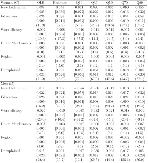
Table 5 includes the estimates of the OLS and unconditional quantile regression bottom of the wage distribution than Blau and Kahn (2004, 2006).

decomposition of changes in wage rates of female and male workers between 1993 and 2006. The numbers suggest that real wages of female workers have increased by 0.071 log points (7.4 percent) at the bottom and by 0.155 log points (16.8 percent) at the top of the distribution. On average, wages of female workers have increased by 0.088 log points (9.2 percent). A large part (41.3 percent) of the wage growth of female workers was due to increases in educational attainment, while changes in work history characteristics worked against that wage growth. The numbers of the unconditional quantile regression decompositions reveal that the contribution of these factors varies considerably across the distribution. While changes in educational attainment explain between 37.4 percent at the 0.9-quantile and 70.6 percent at the median, the contribution of changes in work history characteristics varies from−37.3 percent at the 0.1-quantile to 0.4 percent at the 0.9-quantile. As a result of these variations, less than half of the wage growth of female workers remains unexplained at the median of the distribution, while almost 80 percent of the wage growth remains unexplained at the lower tail of the distribution.

Real wages of male workers increased at the top of the distribution but did not change or even declined moderately lower down the distribution. In contrast to fe-male workers, average wages of fe-male workers did not increase significantly between 1993 to 2006. When looking at the 0.9-quantile of male workers, where a signifi-cant wage growth may be observed, we find that a sizeable part of this growth is explained by increases in educational attainment and union membership. Finally, the decomposition of the selection model suggests that the inclusion of a selection bias correction term only affects the raw differential and the unexplained part of the decomposition equation, while the observed characteristics are mostly unaffected.

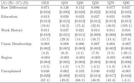
Table 6 includes the decomposition results of changes in the gender wage gap over time (i.e. the differences between Panel A and Panel B of Table 4) which are equal to the decomposition results of gender differences in wage growth (i.e. the differences between Panel C and Panel D of Table 5). On average, the gender wage gap narrowed by 0.071 log points (7.4 percent) between 1993 and 2006, while changes

reached from 0.126 log points (13.4 percent) at the 0.1-quantile to 0.037 log points (3.8 percent) at the 0.9-quantile. The part of the mean differential due to variations in educational attainment is 18.6 percent. Variations in work history characteristics explain 15.7 percent of the gap and another 4.2 percent are attributable to varia-tions in union membership. While variavaria-tions in educational attainment account for only 16.2 percent at the lowest decile, this share increases across the wage distribu-tion to 105.1 percent at the highest decile, suggesting that variadistribu-tions in educadistribu-tional attainment are the major reason for the (relatively small) decline in the gender wage gap at the upper tail of the distribution but do not explain much of the strong decline in the gap at the lower tail of the distribution. Instead, variations in work history characteristics are mainly responsible for narrowing the gender wage gap at the low-est decile. Specifically, 29.3 percent of the changes in the gender wage gap are caused by changes in work history characteristics at the lowest decile. The corresponding share at the highest decile is 27.4 percent.

These results point to substantial heterogeneity with regard to the decline in the gender wage gap across the distribution and the relevance of the factors that are responsible for this decline. While the gender wage gap narrowed by more than 13 percent at the lowest decile, it declined by less than 4 percent at the highest decile. Interestingly, changes in educational attainment did not contribute much to the strong decline in the gender wage gap at the lower tail of the distribution. Instead, variations in work history characteristics were more relevant for this decline. Finally, due to the absence of a number of relevant factors, a large part of the changes in the gender wage gap (up to 70 percent) remains unexplained.

5

Conclusions

Very little is known about the factors that are responsible for distributional changes in the gender wage gap although the factors that explain the gender wage gap do not necessarily affect changes over time and the factors that are responsible for the

decline in the gender wage gap may be different across the wage distribution. This paper investigates changes in the gender wage gap between white men and white women across the wage distribution using Panel Study of Income Dynamics (PSID) data. We take advantage of a newly-developed Blinder-Oaxaca type decomposition for unconditional quantile regression models (Firpo et al., 2007b, 2009) to decompose wage differentials across the entire distribution. We show that this approach allows a consistent decomposition of both changes in the gender wage gap and gender differentials in wage growth across the distribution.

We find that the gender wage gap narrowed by more than 13 percent at the lowest wage decile and by less 4 percent at the highest decile of the wage distribution between 1993 and 2006. The results of the decomposition analysis indicate that the decline in the gender wage gap at the upper tail of the distribution may be attributed entirely to changes in educational attainment in favor of female workers. At the same time, a sizeable part of the decline at the lower tail of the distribution is due to work history changes. On balance, these results point to substantial heterogeneity with regard to the decline in the gender wage gap across the distribution and the relevance of the factors that are responsible for this decline. Moreover, due to the relatively small part of changes in the gap at the bottom of the distribution that is explained by education, it seems likely that the educational success of women did contribute to a reduction in the gender wage gap at the lower end of the distribution since the 1970s. Our findings also suggest that this success could not trigger a strong decline at the top of the distribution until today.

Figures and Tables

Table 1: Wages of Male and Female Workers, 1993 and 2006

Male Female Wage Ratio

1993 2006 Change (%) 1993 2006 Change (%) 1993 2006 Mean 17.15 18.31 6.8 12.23 13.29 8.7 0.713 0.726 Quantile: Q10 6.99 6.70 -4.2 4.55 4.87 7.0 0.651 0.727 Q30 11.06 10.65 -3.7 7.69 8.46 10.0 0.696 0.795 Q50 14.66 14.42 -1.6 10.73 11.33 5.6 0.732 0.786 Q70 19.23 20.00 4.0 14.18 15.26 7.6 0.737 0.763 Q90 28.85 32.97 14.3 20.94 24.04 14.8 0.726 0.729 N 2,047 1,974 1,343 1,681

Table 2: Means and Standard Deviations by Year and Gender

1993 2006

Male Female Male Female Mean SD Mean SD Mean SD Mean SD Hourly wage 17.15 12.64 12.23 8.79 18.31 15.16 13.29 8.73 Educational Attainment

8th grade or below 0.021 0.142 0.009 0.093 0.020 0.142 0.014 0.117 9th to 11th grade 0.112 0.316 0.078 0.269 0.085 0.278 0.056 0.231 12th grade (high school) 0.322 0.467 0.377 0.485 0.294 0.456 0.324 0.468 12 grades plus nonacademic training 0.076 0.265 0.087 0.282 0.085 0.279 0.073 0.260 College but no degree 0.107 0.310 0.115 0.319 0.123 0.329 0.141 0.349 College BA but no advanced degree 0.037 0.190 0.054 0.225 0.047 0.212 0.046 0.210 College and advanced degree 0.324 0.468 0.281 0.450 0.345 0.476 0.345 0.475 Work History Experience 15.0 8.4 13.0 7.5 11.8 7.6 11.9 7.8 Full-time experience 13.4 8.8 10.7 7.4 10.2 7.9 9.6 7.9 Tenure 9.2 8.7 7.7 7.5 9.0 9.2 7.9 8.2 Union member 0.197 0.398 0.132 0.339 0.156 0.363 0.133 0.339 N 2,047 1,974 1,343 1,681

Table 3: OLS Estimates by Gender and Year

Men Women

1993 2006 1993 2006 9th to 11th grade 0.310** 0.490*** 0.133 0.482**

(0.09) (0.11) (0.16) (0.15) 12th grade (high school) 0.485*** 0.605*** 0.472** 0.663***

(0.09) (0.10) (0.15) (0.14) 12 grades plus nonacademic training 0.572*** 0.712*** 0.555*** 0.745***

(0.10) (0.11) (0.16) (0.15) College but no degree 0.649*** 0.853*** 0.714*** 0.816***

(0.09) (0.11) (0.16) (0.14) College BA but no advanced degree 0.705*** 0.971*** 0.840*** 0.951***

(0.10) (0.12) (0.16) (0.15) College and advanced degree 0.972*** 1.197*** 0.983*** 1.159***

(0.09) (0.11) (0.15) (0.14) Experience 0.011 -0.004 0.006 0.009 (0.02) (0.02) (0.01) (0.01) Experience2/100 -0.005 -0.039 -0.049 -0.076 (0.04) (0.06) (0.04) (0.05) Full-time work experience since age 18 0.002 -0.003 0.016 0.011 (0.01) (0.01) (0.01) (0.01) Full-time work experience since age 182/100 -0.011 0.043 -0.006 0.018 (0.04) (0.06) (0.04) (0.04) Tenure 0.047*** 0.038*** 0.061*** 0.043*** (0.00) (0.01) (0.01) (0.00) Tenure2/100 -0.112*** -0.068*** -0.133*** -0.082*** (0.02) (0.02) (0.02) (0.01) Union member 0.095** 0.068* 0.067 0.042 (0.03) (0.03) (0.05) (0.04) Constant 1.658*** 1.752*** 1.273*** 1.264*** (0.11) (0.12) (0.17) (0.15) R2 0.325 0.307 0.375 0.306 N 2,047 1,974 1,343 1,681

NOTE.–The regression model further includes region indicators. Robust standard errors in parentheses.∗p <0.10,∗∗p <0.05,∗∗∗p <0.01.

Table 4: OLS, Heckman and Unconditional Quantile Regression Decomposition of the Gender Wage Gap, 1993 and 2006

1993 (A) OLS Heckman Q10 Q30 Q50 Q70 Q90 Raw Differential 0.352 0.322 0.453 0.388 0.329 0.340 0.352 [0.023] [0.029] [0.064] [0.020] [0.016] [0.015] [0.020] Education 0.002 0.002 -0.007 0.003 0.010 0.015 0.025 [0.009] [0.011] [0.011] [0.008] [0.009] [0.009] [0.011] (0.6) (0.7) (-1.6) (0.9) (3.0) (4.3) (7.0) Work History 0.034 0.033 0.061 0.052 0.042 0.031 0.029 [0.008] [0.008] [0.016] [0.008] [0.007] [0.005] [0.007] (9.7) (10.1) (13.5) (13.4) (12.7) (9.1) (8.3) Union Membership 0.005 0.004 0.013 0.010 0.011 0.007 -0.012 [0.001] [0.001] [0.005] [0.002] [0.002] [0.001] [0.003] (1.3) (1.4) (2.8) (2.6) (3.3) (2.0) (-3.4) Region -0.000 -0.000 -0.000 0.001 0.002 0.004 0.002 [0.003] [0.003] [0.004] [0.003] [0.003] [0.003] [0.004] (-0.1) (-0.1) (-0.1) (0.3) (0.6) (1.1) (0.7) Unexplained 0.311 0.283 0.387 0.321 0.265 0.284 0.308 [0.019] [0.026] [0.063] [0.015] [0.009] [0.009] [0.017] (88.5) (87.9) (85.4) (82.8) (80.4) (83.4) (87.4) 2006 (B) Raw Differential 0.281 0.255 0.327 0.236 0.243 0.263 0.316 [0.025] [0.028] [0.068] [0.019] [0.015] [0.018] [0.041] Education -0.011 -0.011 -0.028 -0.020 -0.017 -0.016 -0.014 [0.009] [0.010] [0.011] [0.008] [0.008] [0.009] [0.010] (-3.9) (-4.2) (-8.4) (-8.5) (-7.2) (-6.1) (-4.5) Work History 0.023 0.022 0.024 0.031 0.028 0.020 0.019 [0.007] [0.007] [0.014] [0.007] [0.006] [0.005] [0.006] (8.1) (8.6) (7.4) (13.0) (11.3) (7.6) (6.0) Union Membership 0.002 0.002 0.005 0.004 0.004 0.003 -0.004 [0.001] [0.001] [0.003] [0.002] [0.002] [0.001] [0.002] (0.6) (0.6) (1.4) (1.6) (1.6) (1.0) (-1.4) Region 0.004 0.004 0.001 0.004 0.005 0.005 0.006 [0.003] [0.003] [0.003] [0.003] [0.003] [0.003] [0.004] (1.3) (1.4) (0.3) (1.6) (2.0) (1.8) (1.8) Unexplained 0.264 0.239 0.325 0.218 0.224 0.252 0.309 [0.022] [0.025] [0.068] [0.015] [0.010] [0.014] [0.039] (93.9) (93.6) (99.3) (92.3) (92.2) (95.7) (98.0) NOTE.–Percentage of total variation explained in parentheses. Analytic standard errors in brackets. Number of observations: 1993: 2,047 men and 1,343 women; 2006: 1,974 men and 1,681 women.

Table 5: OLS, Heckman and Unconditional Quantile Regression Decomposition of Wage Growth between 1993 and 2006, Women and Men

Women (C) OLS Heckman Q10 Q30 Q50 Q70 Q90 Raw Differential 0.088 0.046 0.071 0.096 0.067 0.090 0.155 [0.025] [0.030] [0.077] [0.022] [0.017] [0.016] [0.032] Education 0.036 0.036 0.041 0.042 0.047 0.051 0.058 [0.009] [0.011] [0.012] [0.009] [0.009] [0.010] [0.011] (41.3) (77.9) (57.2) (43.7) (70.6) (57.1) (37.4) Work History -0.009 -0.008 -0.026 -0.011 -0.010 -0.007 0.001 [0.007] [0.008] [0.015] [0.008] [0.007] [0.005] [0.006] (-10.3) (-17.3) (-37.3) (-11.2) (-14.5) (-8.0) (0.4) Union Membership 0.000 0.000 0.001 0.000 0.000 0.000 -0.000 [0.001] [0.001] [0.002] [0.002] [0.002] [0.001] [0.002] (0.0) (0.1) (0.7) (0.4) (0.6) (0.3) (-0.3) Region -0.003 -0.003 0.002 -0.000 -0.003 -0.003 -0.007 [0.003] [0.003] [0.005] [0.003] [0.003] [0.003] [0.005] (-2.9) (-5.6) (2.1) (-0.2) (-4.4) (-3.0) (-4.6) Unexplained 0.063 0.021 0.055 0.064 0.032 0.048 0.104 [0.021] [0.026] [0.076] [0.017] [0.011] [0.011] [0.029] (71.9) (45.0) (77.2) (67.3) (47.6) (53.7) (67.1) Men (D) Raw Differential 0.017 0.005 -0.055 -0.056 -0.019 0.013 0.118 [0.022] [0.024] [0.053] [0.016] [0.014] [0.017] [0.032] Education 0.023 0.023 0.020 0.019 0.020 0.021 0.019 [0.009] [0.010] [0.011] [0.008] [0.008] [0.009] [0.010] (26.2) (49.3) (28.4) (19.4) (29.7) (22.9) (12.4) Work History -0.020 -0.019 -0.063 -0.032 -0.024 -0.018 -0.009 [0.007] [0.008] [0.018] [0.007] [0.006] [0.005] [0.007] (-23.0) (-40.4) (-89.2) (-33.6) (-35.8) (-20.4) (-6.1) Union Membership -0.003 -0.003 -0.007 -0.006 -0.006 -0.004 0.007 [0.001] [0.001] [0.003] [0.002] [0.002] [0.001] [0.002] (-3.3) (-6.0) (-10.5) (-6.1) (-9.4) (-4.4) (4.5) Region 0.001 0.001 0.003 0.002 0.000 -0.002 -0.004 [0.003] [0.003] [0.004] [0.003] [0.003] [0.003] [0.004] (1.6) (2.9) (4.0) (2.5) (0.1) (-2.0) (-2.4) Unexplained 0.015 0.002 -0.007 -0.039 -0.008 0.017 0.105 [0.020] [0.021] [0.055] [0.012] [0.009] [0.013] [0.029] (92.4) (39.7) (13.1) (69.5) (44.4) (126.1) (89.0) NOTE.–See notes to Table 4.

Table 6: OLS and Unconditional Quantile Regression Decomposition of Changes in the Gender Wage Gap

(A)-(B)=(C)-(D) OLS Q10 Q30 Q50 Q70 Q90 Raw Differential 0.071 0.126 0.152 0.086 0.077 0.037 [0.034] [0.093] [0.028] [0.022] [0.024] [0.045] Education 0.013 0.020 0.023 0.027 0.031 0.039 [0.013] [0.015] [0.012] [0.012] [0.013] [0.015] (18.6) (16.2) (15.4) (32.0) (40.0) (105.1) Work History 0.011 0.037 0.021 0.014 0.011 0.010 [0.010] [0.021] [0.011] [0.009] [0.008] [0.009] (15.7) (29.3) (14.1) (16.7) (14.4) (27.4) Union Membership 0.003 0.008 0.006 0.007 0.004 -0.007 [0.002] [0.005] [0.003] [0.003] [0.002] [0.004] (4.2) (6.3) (4.1) (7.9) (5.5) (-20.1) Region -0.004 -0.001 -0.003 -0.003 -0.001 -0.003 [0.004] [0.005] [0.004] [0.004] [0.004] [0.006] (-5.5) (-1.0) (-1.7) (-3.5) (-1.3) (-9.3) Unexplained 0.048 0.062 0.103 0.040 0.032 -0.001 [0.029] [0.093] [0.021] [0.014] [0.017] [0.043] (67.1) (49.2) (68.1) (46.9) (41.4) (-3.1) NOTE.–See notes to Table 4.

References

Albrecht, J, Björklund, A., Vroman, S, 2003. Is There a Glass Ceiling in Sweden?,Journal of Labor Economics21, 145-178.

Antonczyk, D, Fitzenberger, B, Sommerfeld, K, 2010. Rising Wage Inequality, the Decline of Collective Bargaining, and the Gender Wage Gap, IZA Discussion Paper No. 4911.

Arulampalam, W, Booth, AL, Bryan, ML, 2007. Is There a Glass Ceiling over Europe? Exploring the Gender Pay Gap across the Wages Distribution, Industrial and Labor Relations Review 60, 163-186.

Blau, FD, Kahn, LM, 2006. The U.S. Gender Pay Gap in the 1990s: Slowing Convergence,

Industrial and Labor Relations Review 60, 45-66.

Blau, FD, Kahn, LM, 2004. The U.S. Gender Pay Gap in the 1990s: Slowing Convergence, NBER Working Paper No. 10853.

Blau, FD, Kahn, LM, 1997. Swimming Upstream: Trends in the Gender Wage Differential in the 1980s,Journal of Labor Economics15, 1-42.

Blinder, A.S., 1973. Wage Discrimination: Reduced Form and Structural Estimates,Journal of Human Resources8, 436-455.

Borghans, L, Duckworth, AL, Heckman, JJ, ter Weel, B, 2008. The Economics and Psy-chology of Personality Traits,The Journal of Human Resources43, 972-1059.

Bowles, S, Gintis, H, Osborne, M, 2001. The Determinants of Earnings: A Behavioral Approach,Journal of Economic Literature39, 1137-1176.

Cain, GG, 1986. The Economic Analysis of Labor Market Discrimination: A Survey. In: O. Ashenfelter and R. Layard (eds.):Handbook of Labor Economics, Vol. 1, Elsevier Science Publishers BV, pp. 693-785.

Cotton, J, 1988. On the Decomposition of Wage Differentials,The Review of Economics and Statistics70, 236-243.

DiNardo, J, Fortin, NM, Lemieux, T, 1996. Labor Market Institutions and the Distribution of Wages, 1973-1992: A Semiparametric Approach,Econometrica64, 1001-1044.

Elder, TE, Goddeeris, JH, Haider, SJ, 2010. Unexplained Gaps and Oaxaca-Blinder De-compositions,Labour Economics 17, 284-290.

Firpo, S, Fortin, NM, Lemieux, T, 2009. Unconditional Quantile Regressions,Econometrica

77, 953-973.

Firpo, S, Fortin, NM, Lemieux, T, 2007a. Decomposing Wage Distributions using Recen-tered Influence Function Regressions. Working Paper, Department of Economics, Uni-versity of British Columbia.

Firpo, S, Fortin, NM, Lemieux, T, 2007b. Unconditional Quantile Regressions. NBER Tech-nical Working Paper No. 339.

Fortin, NM, 2008. The Gender Wage Gap among Young Adults in the United States: The Importance of Money versus People,The Journal of Human Resources43, 884-918.

Fortin, NM, Lemieux, T, Firpo, S, 2010. Decomposition Methods in Economics. In: Ashen-felter, O, Card, D (eds.): Handbook of Labor Economics, Vol. 4a, Elsevier Science Pub-lishers BV, forthcoming.

Gardeazabal, J, Ugidos, A, 2004. More on Identification in Detailed Wage Decompositions,

The Review of Economics and Statistics86, 1034-1036.

García, J, Hernández, PJ, López-Nicolás, A, 2001. How Wide is the Gap? An Investigation of Gender Wage Differences Using Quantile Regressions,Empirical Economics 26, 149-167.

Gelbach, JB, 2002. Identified Heterogeneity in Detailed Wage Decompositions. Unpublished Working Paper.

Gosling, A, Machin, S, Meghir, C, 2000. The Changing Distribution of Male Wages in the U.K.,Review of Economic Studies67, 635-666.

Gupta, ND, Oaxaca, RL, Smith, N, 2006. Swimming Upstream, Floating Downstream: Comparing Women’s Relative Wage Progress in the United States and Denmark,Journal Industrial and Labor Relations Review 59, 243-266.

Heckman, J, Strixrud, J, Urzua, S, 2006. The Effects of Cognitive and Noncognitive Abilities on Labor Market Outcomes and Social Behavior,Journal of Labor Economics24, 411-482.

Horrace, WC, Oaxaca, RL, 2001. Inter-Industry Wage Differentials and the Gender Wage Gap: An Identification Problem,Industial and Labor Relations Review 54, 611-618.

Jann, B, 2008. The Blinder-Oaxaca Decomposition for Linear Regression Models,The Stata Journal8, 453-479.

Jones, FL, 1983. On Decomposing the Wage Gap: A Critical Comment on Blinder’s Method,The Journal of Human Resources18, 126-130.

Jones, FL, Kelley, J, 1984. Decomposing Differences Between Groups. A Cautionary Note on Measuring Discrimination,Sociological Methods and Research12, 323-343.

Judge, TA, Tippie, HB, Bono, JH, 2001. Relationship of Core evaluations Traits - Self-esteem, Generalized Self-efficacy, Locus of Control, and Emotional Stability - with Job Satisfaction and Job Performance: A Meta-Analysis,Journal of Applied Psychology 86, 80-92.

Juhn, C, Murphy, KM, Pierce, B, 1993. Wage Inequality and the Rise in Returns to Skill,

Journal of Political Economy101, 410-442.

Kuhn, P, Weinberger, C, 2005. Leadership Skills and Wages,Journal of Labor Economics

Machado, JAF, Mata, J, 2005. Counterfactual Decomposition of Changes in Wage Distri-butions using Quantile Regression,Journal of Applied Econometrics20, 445-465.

Manning, A, Swaffield, J, 2005. The Gender Gap in Early-Career Wage Growth, CEP Discussion Paper No. 700.

Melly, B, 2005. Decomposition of Differences in Distribution Using Quantile Regression,

Labour Economics 12, 577-590.

Neuman, S, Oaxaca, RL, 2004. Wage Decomposition with Selectivity-Corrected Wage Equa-tions: A Methodological Note,Journal of Economic Inequality 2, 3-10.

Neumark, D, 1988. Employers’ Discriminatory Behavior and the Estimation of Wage Dis-crimination,The Journal of Human Resources23, 279-295.

Oaxaca, RL, 1973. Male-Female Wage Differentials in Urban Labor Markets,International Economic Review 14, 693-709.

Oaxaca, RL, Ransom, M, 1994. On Discrimination and the Decomposition of Wage Differ-entials,Journal of Econometrics 61, 5-21.

Oaxaca, RL, Ransom, M, 1999. Identification in Detailed Wage Decompositions,The Re-view of Economics and Statistics81, 154-157.

O’Neill, JA, 2003. The Gender Gap in Wages, circa 2000,American Economic Review -AEA Papers and Proceedings93, 309-314.

O’Neill, J, Polachek, S, 1993. Why the Gender Gap in Wages Narrowed in the 1980s,

Journal of Labor Economics11, 25-33.

Pissarides, C, Garibaldi, P, Olivetti, C, Petrongolo, B, Wasmer, E, 2005. The Evoluation of the Gender Wage Gap in the U.S. In: T. Boeri, D. del Boca and C. Pissarides (eds.):

Women at Work - An Economic Perspective. Oxford University Press, pp. 66-67.

Reimers, CW, 1983. Labor Market Discrimination Against Hispanic and Black Men,The Review of Economics and Statistics65, 570-579.

Rothe, C, 2010a. Nonparametric Estimation of Distributional Policy Effects, Journal of Econometrics 155, 56-70.

Rothe, C, 2010b. Decomposing Counterfactual Distributions, Toulouse School of Eco-nomics, mimeo.

Waddell, GR, 2005. Labor Market Consequences of Poor Attitude and Low Self-Esteem in Youth,Economic Inquiry 44, 69-97.

Wellington, AJ, 1993. Changes in the Male/Female Wage Gap, 1976-85,The Journal of Human Resources28, 383-411.

Yun, M-S, 2005. A Simple Solution to the Indentification Problem in Detailed Wage De-compositions,Economic Inquiry43, 766-772.

Appendix

Table A1: Unconditional Quantile Regression Estimates – Male Workers, 1993 Q10 Q30 Q50 Q70 Q90 9th to 11th grade 0.948** 0.458** 0.286*** 0.126 0.141**

(0.349) (0.141) (0.084) (0.085) (0.053) 12th grade (high school) 1.148*** 0.627*** 0.407*** 0.246** 0.236***

(0.343) (0.134) (0.080) (0.086) (0.066) 12 grades plus nonacademic training 1.166** 0.788*** 0.505*** 0.326*** 0.298***

(0.357) (0.145) (0.092) (0.097) (0.084) College but no degree 1.394*** 0.843*** 0.599*** 0.424*** 0.281***

(0.343) (0.139) (0.087) (0.094) (0.074) College BA but no advanced degree 1.423*** 0.877*** 0.678*** 0.498*** 0.351** (0.345) (0.152) (0.111) (0.120) (0.112) College and advanced degree 1.486*** 1.067*** 0.902*** 0.795*** 0.840***

(0.342) (0.134) (0.081) (0.089) (0.085) Experience 0.032 0.024 0.020 -0.011 -0.038

(0.032) (0.020) (0.015) (0.016) (0.023) Experience2/100 -0.108 -0.067 -0.015 0.062 0.190* (0.090) (0.057) (0.041) (0.050) (0.083) Full-time work experience since age 18 -0.016 -0.005 -0.008 0.017 0.046* (0.026) (0.017) (0.013) (0.014) (0.020) Full-time work experience since age 182/100 0.082 0.029 -0.002 -0.067 -0.184* (0.078) (0.052) (0.039) (0.047) (0.078) Tenure 0.066*** 0.061*** 0.041*** 0.032*** 0.026** (0.009) (0.006) (0.005) (0.005) (0.008) Tenure2/100 -0.163*** -0.144*** -0.090*** -0.061** -0.064 (0.032) (0.021) (0.018) (0.020) (0.033) Union member 0.230*** 0.172*** 0.186*** 0.037 -0.124* (0.049) (0.045) (0.041) (0.043) (0.050) Constant 0.234 1.216*** 1.777*** 2.282*** 2.692*** (0.361) (0.154) (0.102) (0.108) (0.111) R2 0.136 0.237 0.276 0.226 0.153 N 2047 2047 2047 2047 2047

NOTE.–The regression model further includes region indicators. Robust standard errors in parentheses.∗p <0.10,∗∗p <0.05,∗∗∗p <0.01.

Table A2: Unconditional Quantile Regression Estimates – Male Workers, 2006 Q10 Q30 Q50 Q70 Q90 9th to 11th grade 1.460*** 0.491*** 0.300*** 0.110* 0.063

(0.368) (0.130) (0.076) (0.055) (0.063) 12th grade (high school) 1.543*** 0.696*** 0.458*** 0.213*** 0.061

(0.351) (0.117) (0.065) (0.051) (0.058) 12 grades plus nonacademic training 1.557*** 0.737*** 0.560*** 0.433*** 0.300** (0.365) (0.129) (0.084) (0.083) (0.105) College but no degree 1.752*** 0.949*** 0.751*** 0.517*** 0.249** (0.354) (0.121) (0.076) (0.075) (0.080) College BA but no advanced degree 1.965*** 1.010*** 0.917*** 0.696*** 0.298* (0.354) (0.132) (0.093) (0.111) (0.122) College and advanced degree 1.926*** 1.136*** 1.014*** 1.000*** 0.837***

(0.348) (0.117) (0.068) (0.068) (0.098) Experience -0.010 0.004 -0.009 -0.008 -0.034

(0.032) (0.018) (0.017) (0.021) (0.033) Experience2/100 -0.045 -0.088 -0.015 -0.008 0.085

(0.115) (0.071) (0.068) (0.076) (0.123) Full-time work experience since age 18 0.006 -0.009 -0.004 -0.001 0.010

(0.026) (0.015) (0.015) (0.018) (0.030) Full-time work experience since age 182/100 0.037 0.089 0.042 0.015 -0.026

(0.101) (0.063) (0.061) (0.071) (0.117) Tenure 0.057*** 0.046*** 0.032*** 0.024*** 0.009 (0.011) (0.006) (0.006) (0.007) (0.009) Tenure2/100 -0.126*** -0.093*** -0.049** -0.019 0.021 (0.032) (0.019) (0.019) (0.023) (0.030) Union member 0.174* 0.202*** 0.187*** 0.055 -0.226*** (0.069) (0.044) (0.046) (0.056) (0.063) Constant 0.008 1.378*** 1.941*** 2.467*** 3.310*** (0.358) (0.131) (0.090) (0.088) (0.117) R2 0.111 0.214 0.233 0.241 0.138 N 1974 1974 1974 1974 1974

Table A3:Unconditional Quantile Regression Estimates – Female Workers, 1993 Q10 Q30 Q50 Q70 Q90 9th to 11th grade 0.403 0.588*** 0.162 -0.121 -0.109

(0.718) (0.133) (0.092) (0.069) (0.058) 12th grade (high school) 1.321 1.045*** 0.368*** 0.031 -0.090* (0.689) (0.107) (0.078) (0.061) (0.045) 12 grades plus nonacademic training 1.218 1.141*** 0.450*** 0.128 -0.081

(0.698) (0.129) (0.098) (0.080) (0.054) College but no degree 1.550* 1.256*** 0.582*** 0.269** 0.140

(0.693) (0.118) (0.095) (0.082) (0.075) College BA but no advanced degree 1.493* 1.366*** 0.890*** 0.499*** 0.163

(0.691) (0.126) (0.113) (0.126) (0.119) College and advanced degree 1.509* 1.481*** 0.936*** 0.647*** 0.510***

(0.687) (0.104) (0.080) (0.073) (0.076) Experience 0.053 0.018 -0.006 -0.010 -0.028

(0.034) (0.021) (0.017) (0.015) (0.018) Experience2/100 -0.198 -0.103 -0.044 0.003 0.080

(0.122) (0.061) (0.050) (0.048) (0.062) Full-time work experience since age 18 -0.019 0.008 0.032* 0.044** 0.047** (0.029) (0.020) (0.016) (0.014) (0.015) Full-time work experience since age 182/100 0.138 0.055 -0.026 -0.118* -0.148**

(0.119) (0.066) (0.054) (0.051) (0.057) Tenure 0.131*** 0.076*** 0.060*** 0.033*** 0.002 (0.018) (0.010) (0.007) (0.007) (0.009) Tenure2/100 -0.390*** -0.193*** -0.135*** -0.032 0.059 (0.071) (0.041) (0.026) (0.027) (0.043) Union member 0.097 0.094 0.054 0.059 0.020 (0.084) (0.068) (0.062) (0.065) (0.086) Constant -0.749 0.349* 1.517*** 2.161*** 2.833*** (0.723) (0.144) (0.110) (0.098) (0.099) R2 0.166 0.243 0.292 0.297 0.188 N 1343 1343 1343 1343 1343

Table A4:Unconditional Quantile Regression Estimates – Female Workers, 2006 Q10 Q30 Q50 Q70 Q90 9th to 11th grade 1.039* 0.729*** 0.260** 0.172* -0.020

(0.492) (0.111) (0.085) (0.080) (0.063) 12th grade (high school) 1.430** 0.980*** 0.428*** 0.188*** 0.029

(0.459) (0.069) (0.057) (0.054) (0.063) 12 grades plus nonacademic training 1.401** 1.102*** 0.571*** 0.328*** 0.184

(0.472) (0.089) (0.076) (0.076) (0.095) College but no degree 1.616*** 1.191*** 0.594*** 0.263*** 0.184* (0.461) (0.079) (0.067) (0.065) (0.091) College BA but no advanced degree 1.611*** 1.202*** 0.719*** 0.522*** 0.356** (0.470) (0.115) (0.096) (0.099) (0.133) College and advanced degree 1.733*** 1.450*** 0.947*** 0.705*** 0.723***

(0.457) (0.071) (0.060) (0.061) (0.091) Experience 0.019 0.001 0.001 0.002 -0.017

(0.030) (0.016) (0.013) (0.014) (0.019) Experience2/100 -0.081 -0.053 -0.055 -0.034 0.008

(0.116) (0.051) (0.043) (0.048) (0.053) Full-time work experience since age 18 0.014 0.010 0.006 0.014 0.028

(0.024) (0.013) (0.011) (0.012) (0.018) Full-time work experience since age 182/100 -0.002 0.013 0.035 -0.016 -0.050

(0.102) (0.049) (0.041) (0.045) (0.056) Tenure 0.086*** 0.054*** 0.036*** 0.025*** 0.022* (0.010) (0.006) (0.006) (0.006) (0.010) Tenure2/100 -0.224*** -0.106*** -0.047* -0.018 -0.010 (0.031) (0.020) (0.018) (0.021) (0.040) Union member 0.071 0.058 0.087 0.116* -0.182* (0.070) (0.055) (0.050) (0.059) (0.084) Constant -0.575 0.751*** 1.635*** 2.163*** 2.851*** (0.455) (0.072) (0.062) (0.060) (0.080) R2 0.125 0.216 0.253 0.214 0.123 N 1681 1681 1681 1681 1681

Table A5:Heckman Selection Estimates by Gender and Year – Wage Equation

Men Women

1993 2006 1993 2006 9th to 11th grade 0.304** 0.494*** 0.099 0.469**

(0.095) (0.109) (0.162) (0.150) 12th grade (high school) 0.472*** 0.610*** 0.428** 0.641***

(0.092) (0.103) (0.152) (0.140) 12 grades plus nonacademic training 0.556*** 0.709*** 0.508** 0.727***

(0.102) (0.115) (0.158) (0.150) College but no degree 0.636*** 0.853*** 0.665*** 0.792***

(0.095) (0.106) (0.156) (0.143) College BA but no advanced degree 0.692*** 0.972*** 0.792*** 0.940***

(0.103) (0.116) (0.165) (0.152) College and advanced degree 0.954*** 1.195*** 0.930*** 1.138***

(0.095) (0.108) (0.154) (0.141) Experience 0.013 -0.002 0.006 0.008

(0.016) (0.017) (0.014) (0.013) Experience2/100 -0.006 -0.040 -0.044 -0.070

(0.045) (0.062) (0.046) (0.048) Full-time work experience since age 18 0.001 -0.004 0.015 0.011

(0.014) (0.015) (0.012) (0.010) Full-time work experience since age 182/100 -0.009 0.042 -0.009 0.013

(0.041) (0.058) (0.045) (0.043) Tenure 0.044*** 0.033*** 0.051*** 0.037*** (0.005) (0.005) (0.007) (0.006) Tenure2/100 -0.103*** -0.055** -0.104*** -0.067*** (0.017) (0.017) (0.026) (0.017) Union member 0.094** 0.060 0.055 0.033 (0.030) (0.031) (0.044) (0.039) Constant 1.696*** 1.782*** 1.414*** 1.344*** (0.110) (0.118) (0.174) (0.150) Inverse Mill’s ratio -0.083* -0.105*** -0.091*** -0.065* (0.043) (0.037) (0.029) (0.036)

N 2,262 2,181 2,271 2,458

Table A6: Heckman Selection Estimates by Gender and Year – Participation Equation

Men Women

1993 2006 1993 2006 9th to 11th grade 0.449* 0.020 0.506 0.301 (0.218) (0.322) (0.263) (0.221) 12th grade (high school) 0.778*** -0.084 0.844*** 0.700***

(0.221) (0.297) (0.252) (0.207) 12 grades plus nonacademic training 0.974*** 0.276 0.821** 0.583* (0.260) (0.325) (0.269) (0.233) College but no degree 0.763** 0.126 0.903*** 0.773***

(0.248) (0.332) (0.264) (0.217) College BA but no advanced degree 0.675* 0.074 0.811** 0.330

(0.324) (0.359) (0.276) (0.240) College and advanced degree 1.060*** 0.306 0.982*** 0.636** (0.233) (0.303) (0.255) (0.209) Experience -0.086* -0.080* 0.009 0.032

(0.043) (0.040) (0.024) (0.025) Experience2/100 0.124 0.080 -0.145 -0.201* (0.122) (0.133) (0.086) (0.080) Full-time work experience since age 18 0.073* 0.041 0.032 0.001

(0.037) (0.033) (0.023) (0.022) Full-time work experience since age 182/100 -0.170 0.003 0.087 0.137

(0.112) (0.124) (0.097) (0.079) Tenure 0.224*** 0.246*** 0.234*** 0.236*** (0.027) (0.029) (0.017) (0.014) Tenure2/100 -0.531*** -0.618*** -0.698*** -0.638*** (0.073) (0.076) (0.083) (0.047) Union member 0.066 0.529* 0.395** 0.481** (0.193) (0.256) (0.141) (0.163) Married 0.332* 0.210 -0.691*** -0.636*** (0.129) (0.115) (0.088) (0.083) Number of children -0.015 0.136* -0.086** -0.067* (0.055) (0.054) (0.028) (0.028) Constant -0.054 0.624 -0.835** -0.462* (0.319) (0.354) (0.281) (0.228) N 2,262 2,181 2,271 2,458