Advanced modulation techniques for scaling up multiuser MIMO communications.

(1)

Advanced Modulation Techniques For Scaling Up

Multiuser MIMO Communications

J.C. De Luna Ducoing

Submitted for the Degree of Doctor of Philosophy

from the University of Surrey

Institute for Communication Systems Faculty of Engineering and Physical Sciences

University of Surrey Surrey, U.K.

January 2018

c

(2)

(3)

Declaration of Originality

This thesis and the work to which it refers are the results of my own efforts. Any ideas, data, images or text resulting from the work of others (whether published or unpub-lished) are fully identified as such within the work and attributed to their originator in the text, bibliography or in footnotes. This thesis has not been submitted in whole or in part for any other academic degree or professional qualification. I agree that the University has the right to submit my work to the plagiarism detection service Turnit-inUK for originality checks. Whether or not drafts have been so-assessed, the University reserves the right to require an electronic version of the final document (as submitted) for assessment as above.

Juan Carlos De Luna Ducoing September 29, 2017

(4)

Abstract

Multiuser multiple-input multiple-output (MU-MIMO) has the potential to substan-tially increase the uplink network efficiency by multiplexing the user terminals’ (UTs) transmissions in the spatial domain. However, demultiplexing the transmissions at the network side, known as MU-MIMO detection, can become a considerable signal pro-cessing challenge, especially in cases with a high spatial user load. During the last two decades, the MIMO detection problem has been extensively studied, and many receiver designs have been proposed that offer very good tradeoffs in complexity vs. performance. Nevertheless, MU-MIMO detection still presents challenges in signal processing scala-bility in the number of antennas and modulation order. We revisit this problem but through an alternative method of joint transmitter and receiver design. Two approaches that exhibit near-optimal reliability and low complexity are presented:

First, a technique that uses real-valued modulation in fully- and over-loaded cases in large MU-MIMO systems, where there are equal or more UTs than service antennas. It is seen that the use of real constellations with a widely linear equaliser benefits from an increased spatial diversity gain over complex constellations with a linear equaliser. Moreover, a likelihood ascent search (LAS) algorithm post-processing stage is applied to further improve the error performance. Computer simulations show remarkable results for large MU-MIMO sizes in uncoded or coded cases.

Second, recognising that real-valued modulation offers poor modulation efficiency, a real-complex hybrid modulation (RCHM) scheme is proposed, where a mix of real- and complex-valued symbols are interleaved in the spatial and temporal domains. It is seen that RCHM combines the merits of real and complex modulations and enables the ad-justment of the diversity-multiplexing tradeoff. Through the system outage probability analysis, the optimal ratio of the number real-to-complex symbols, as well as their op-timal power allocation, is found for the RCHM pattern. Furthermore, reliability is improved with a small expense in complexity through the use of a successive interfer-ence cancellation (SIC) stage. Results are validated through the mathematical analysis of the average bit error rate and through computer simulations considering single and multiple base station scenarios, which show SNR gains over conventional approaches in excess of 5 dB at 1% BLER.

The results suggest that an expense in complexity is not the only way to improve error performance, but near-optimal reliability is also possible using simple techniques through a reduction in the multiplexing gain. Therefore, rather than a two-way complexity vs. performance tradeoff in MU-MIMO detection, a three-way tradeoff may be more appropriate, and is roughly expressed in the following statement:

“Low complexity, high reliability, high multiplexing gain: choose two.”

Key words: Multiuser multiple-input multiple-output (MU-MIMO), detection, widely

linear (WL) receiver, real-complex hybrid modulation (RCHM), successive interference cancellation (SIC), likelihood ascent search (LAS).

(5)

Acknowledgements

First and foremost, I would like to thank my principal supervisor, Dr. Yi Ma, for his guidance throughout my PhD program journey. I truly thank him for his near-absolute availability, contagious enthusiasm for research, utter patience, profound dedication to his students and for setting an example of how to be a successful researcher.

I am also grateful to my co-supervisors: Dr. Na Yi for her support and for sharing her knowledge and experience; and Prof. Rahim Tafazolli for his leadership and for allowing me the privilege of having been a part of the prestigious Institute for Communication Systems (ICS). To my three supervisors, I am forever indebted.

I also thank my colleagues and teammates at the ICS for their support, helpful discus-sions, and for their camaraderie that comes from being in the same boat as me.

On a personal note, I would like to thank my friends and family, including, but not limited to: my mother and father for their boundless love and unfailing support; my son Carlos and my daughter Mariana, who are my pride and joy, I take this opportunity to remind them to always follow their dreams; and last but not least, my wife Sonia, for her endless love and encouragement, any accomplishment is as much hers as it is mine.

(6)

List of Figures

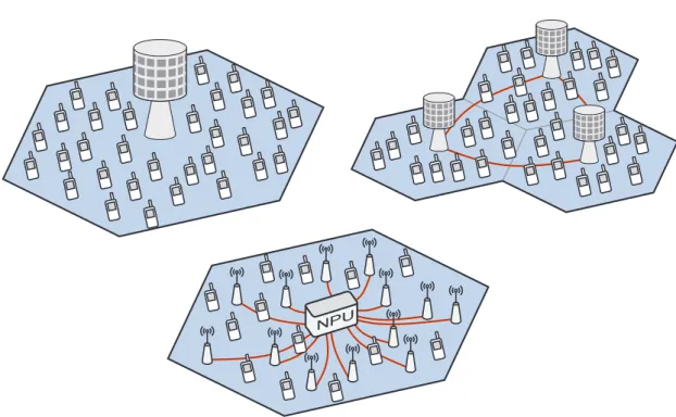
1.1 User-dense MU-MIMO network architecture types. Clockwise from upper-left: single-base station MU-MIMO; multiple cooperating BS scenario; and cell-free MU-MIMO, where ‘NPU’ refers to network processing unit. . 2 2.1 Uplink system model diagram. K UTs communicate over an MU-MIMO

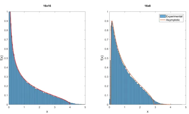
channel to a BS or set of cooperating BSs with a total ofMservice antennas. 11 2.2 Mar˘cenko-Pastur asymptotic distribution with λ= 1 (left) and λ = 0.5

(right), compared to the empirical eigenvalue distribution of a square 16×16 (left), and rectangular 16×8 (right) matrices. . . 15 2.3 Distortion of the transmit constellation due to the MIMO channel and

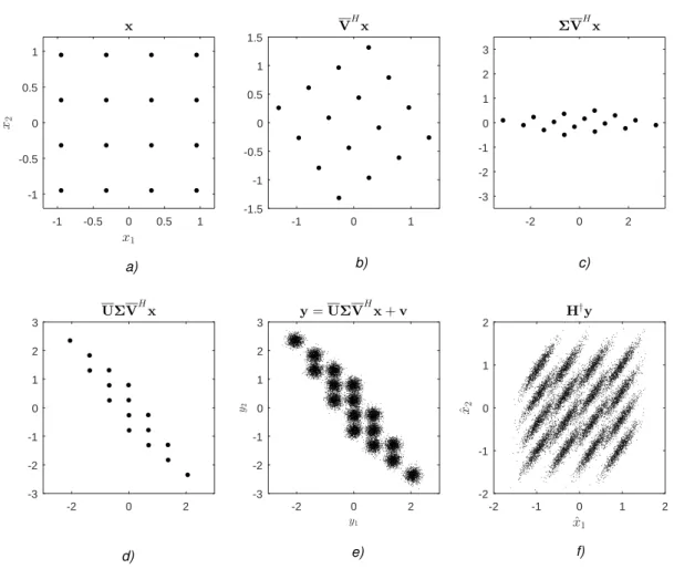
Gaussian noise. Subfigures a) shows the undistorted transmit constella-tion;b)the constellation is rotated by the effect of the unitary matrixVH;

c) the constellation is compressed or expanded along each axis according to the singular values;d) is rotated once more due to the unitary matrix

U; e) white Gaussian noise is added, corresponding to 15 dB SNR; and finallyf ) the effect of ZF processing makes the noise correlated. . . 17 2.4 MIMO 2×2 optimal decision regions. . . 18 2.5 Conceptual diagram of the sphere decoder algorithm of a 4×4 MIMO

system with 4-ABPSK modulation with constellation points {-3,-1,1,3}; R denotes the radius of the hypersphere. . . 21 2.6 Example sphere decoding algorithm running time vs. SNR for the

Fincke-Pohst and Schnorr-Euchner variants. . . 22 2.7 True ML vs. ML approximation in (2.17) for an i.i.d. flat Rayleigh fading

channel, for different MIMO sizes. . . 24 2.8 16-QAM constellation (left), and 4-ABPSK constellation (right), where

adenotes the amplitude factor, I and Q the inline and quadrature axes, respectively. . . 28

(10)

List of Figures v

2.9 Lattice generated by the basisB = [ [1,1]T,[3,1]T ], and the basis after reduction ˜B= [ [1,1]T,[−1,1]T ], which has a lower orthogonality defect. 30 2.10 Primal lattice with basisB= [ [1,1]T,[3,1]T ], and dual lattice with basis

B? = [ [−0.5,1.5]T,[0.5,−0.5]T ]. . . 32 2.11 Uncoded BER performance versus number of antennas when M = K of

lattice reduction techniques with QPSK modulation at 20 dB Eb/N0, for 16×16 through 128×128 antennas, for a frequency-flat independent and identically distributed (i.i.d.) Rayleigh fading channel. . . 34 2.12 BER vs. Eb/N0 plot for an uncoded 4×4 MIMO with QPSK

modu-lation for SDR and other other detection techniques. Fading channel is frequency-flat i.i.d. Rayleigh. . . 37 2.13 BER vs. algorithm running time whilst using Matlab of conventional

MIMO detection algorithms for QPSK modulation and 12 dB Eb/N0 for a flat i.i.d. Rayleigh fading channel. The left point of each segment shows the results for 4×4 MIMO, while the right corresponds to 8×8 MIMO.The results are for uncoded systems. . . 38 2.14 Conceptual diagram of LAS algorithm. Starting from the initial vector,

the algorithm searches among its neighbours for those are closer to the received vector. . . 41 2.15 Example case where the LAS algorithm stops at a local, rather than global

minimum. . . 42 2.16 Average BER vs. Eb/N0 of uncoded BPSK-modulated MIMO with LAS

detection for different system sizes, for a flat i.i.d. Rayleigh channel. The figure shows that the error performance improves with the MIMO size. . . 44 2.17 Uncoded BER performance versus Eb/N0 of ZF-LAS and MMSE-LAS

with QPSK modulation for different numbers of antennas. It is shown that MMSE-LAS converges to near-optimal performance as the number of antennas increases, while ZF-LAS does not. The fading channel is frequency-flat i.i.d. Rayleigh. . . 45 2.18 Average BER vs. Eb/N0 of MMSE-TS vs. MMSE-LAS for different

MIMO sizes. The results are for uncoded systems with a flat i.i.d. Rayleigh channel. . . 46 2.19 BER vs. Eb/N0 for PDA (5 iterations) and damped BP (20 iterations,

with a 0.4 damping factor) for different MIMO sizes with QPSK modula-tion, for uncoded systems with a frequency-flat Rayleigh fading channel. . 47 2.20 BER vs. number of antennas (with M = K) of large MIMO detection

algorithms for QPSK modulation and 10 dB Eb/N0, with a flat i.i.d. Rayleigh fading channel, for uncoded systems. . . 50

(11)

List of Figures vi

3.1 Block diagram of MU-MIMO with a WLZF-LAS receiver. The FEC, MOD and FEC−1 blocks refer to the channel coding, amplitude binary-phase shift keying (ABPSK) modulators and channel decoding, respectively. 54 3.2 The diversity-multiplexing tradeoff (G_div, G_mux) of WLZF with real

mod-ulations and ZF with complex modulation. . . 60 3.3 BER vs. Eb/N0 in a fully-loaded system for ZF and WLZF forL={2,4},

and WLZF for L = {2,4,8,16} with 128×128 antennas. Also includes results for ZF using QPSK with 128×64 antennas. The results are for uncoded systems with a frequency-flat block Rayleigh fading channel. . . 65 3.4 BER vs. Eb/N0 in fully-loaded 128×128 MIMO for ZF-LAS with L =

{2,4} and WLZF-LAS with L = {2,4,6,16}. Results are for uncoded systems with an i.i.d. Rayleigh fading channel. . . 67 3.5 BER vs. Eb/N0 for WLZF and WLZF-LAS using 4-ABPSK

modu-lation with M = 64. Plots are shown for an uncoded system with α={1,1.5,1.875,2}, with a flat i.i.d. Rayleigh fading channel. . . 67 3.6 BER vs. Eb/N0 for WLZF and WLZF-LAS using 4-ABPSK modulation

with M = 64. Plots are shown for a 1_/₃_{-rate turbo-coded system with}

α={1,1.5}, and a frequency-flat Rayleigh fading channel. . . 68

4.1 Block diagram of RCHM-MIMO. The CRC, FEC, MOD, EQ/IC, DE-MOD, FEC−1, and CRC−1 blocks refer to the CRC encoding, channel coding, real-complex hybrid modulation (RCHM) modulators, equalisa-tion/interference cancellation, demodulators, channel decoding, and CRC detection, respectively. The HS block refers to the channel emulation, for

only the streams that passed the CRC check. . . 72 4.2 RCHM example pattern forα= 1/2. . . 74 4.3 The spatial diversity-multiplexing tradeoff (G_div, G_mux) for real, complex

and RCHM-modulated MU-MIMO using the WLZF channel equaliser. . . 79 4.4 Surface plot ofP_out(4.7) vs. γr andKc in (4.12). The plot shows thatP

(4.7) out

is convex, s.t. the condition in (4.13). Some irregularities exist, as shown in the plot, but are not minimums. . . 80 4.5 Surface and contour plots of γ0, the minimum required SNR vs. Kc and

target rate R in (4.19). The plot shows thatγ0 is a convex function ofKc. 82

4.6 Minimum SNR required for RCHM-MIMO to achieve a 1% outage prob-ability, for real, complex and RCHM modulation. The plots are for a system with 20 BS antennas and three system loading scenarios with K={20,18,10}. The curves for RCHM-MIMO use the outage probabil-ity (4.19). . . 83

(12)

List of Figures vii

4.7 State transition diagram for the BER analysis considering the WL-SL-SIC receiver. TheSk, k ∈[0, K] nodes denote the transition states, whereas

theEk,k∈[0, K] nodes denote the states when the algorithm has stopped. 87

4.8 Average-BER as a function of Eb/No for uncoded 20-by-20 RCHM-MIMO system. The curves show the results obtained by simulations and by the theoretical approach in Section 4.3.2, and are compared to the approx-imate ML bound in (2.17). The fading channel is a frequency-flat i.i.d. block Rayleigh. . . 93 4.9 Average-BER as a function of Eb/No for uncoded RCHM-MIMO system

of different sizes, from 12×12 through 128×128, and each for 3, 4 and 6 average bits/symbol. The fading channel is flat i.i.d. block Rayleigh. Also included are the SISO AWGN lower bounds. . . 94 4.10 Performance comparison between uncoded RCHM-MIMO and baselines.

For baseline techniques, 16-QAM is utilised as an example; and corre-spondingly the RCHM-MIMO technique adopts 4 bits/symbol. The fad-ing channel is a flat i.i.d. block Rayleigh. . . 95 4.11 Average number of iterations of the WL-SL-SIC receiver vs. Eb/No for

various RCHM-MIMO sizes, and each for 3,4 and 6 average bits/symbol. The results are for uncoded systems with a flat i.i.d. block Rayleigh fading channel. . . 96 4.12 Average-BER as a function of SNR for uncoded 20-by-20 RCHM-MIMO

system with respect to the number of iterations. The spectral efficiency is 4 bit/symbol, and the fading channel is a frequency-flat i.i.d. block Rayleigh. . . 97 4.13 Throughput in bit/s/Hz/UT for 24-by-24 RCHM-MIMO with different

real-to-complex ratios: α = 2/1,1/1,1/2, 1/3. The modulations are hy-brid of 16-ABPSK and 256-QAM. The results are for uncoded systems with a frequency-flat i.i.d. block Rayleigh fading channel. . . 98 4.14 Average-BLER of 1/3- and 5/6-rate turbo coded RCHM-MIMO in

20-by-20 MU-MIMO systems perfect and imperfect CSI. The fading channel is a flat i.i.d. block Rayleigh. . . 99 4.15 Three cooperating BSs in an edge-excited cell setup, used for the

simula-tion scenario 5. . . 100 4.16 Average BLER vs. UT transmit power (dBm/bit) with the cell-excited

setup. The results compare RCHM-MIMO vs. baselines. . . 101 4.17 The average BLER vs. UT transmit power in dBm/bit of each individual

UT and overall average of all UTs for RCHM-MIMO (left) and conven-tional MU-MIMO (right). . . 102

(13)

List of Figures viii

4.18 Average BLER vs. Eb/N0 of RCHM-MIMO vs the baselines in the cell-excited setup, when implementing power control. . . 103 4.19 The average BLER vs. Eb/N0 of each individual user and overall average

of all UTs, for RCHM-MIMO (left) and conventional MU-MIMO (right), when implementing power control. . . 103 5.1 Conceptual Venn diagram of the three-way tradeoff in MU-MIMO

detec-tion between high reliability, low complexity and high multiplexing gain, which show where some detection approaches fall within the tradeoff. Note that ‘Asym MIMO’ refers to asymmetric MIMO. . . 109

(14)

List of Tables

2.1 Summary of conventional detection methods. . . 39

(15)

List of Abbreviations

3GPP 3rd Generation Partnership Project ABPSK Amplitude binary-phase shift keying AMC Adaptive modulation and coding APP A posteriori probability

ASK Amplitude shift keying

AWGN Additive white Gaussian noise

BER Bit error rate

BI-GDFE Block-iterative generalised decision feedback equaliser

BLER Block error rate

BP Belief propagation

BPSK Binary phase shift keying

BS Base station

CDF Cumulative distribution function CDMA Code division multiple access

CDSA Control-data separation architecture

CLT Central limit theorem

CQI Channel quality indicator

CRC Cyclic redundancy check

CSI Channel state information

CVP Closest vector problem

DFE Decision feedback equaliser DMT Diversity-multiplexing tradeoff

(16)

List of Abbreviations xi

DoF Degrees of freedom

ELR Element-based lattice reduction

EPA Extended Pedestrian-A

FCSD Fixed-complexity sphere decoder

FEC Forward error correction

GAI Gaussian approximation of interference

GMSK Gaussian minimum shift keying

GSM Global system for mobile communication i.i.d. Independent and identically distributed

ILS Integer least squares

IoT Internet of things

LAS Likelihood ascent search

LLL Lenstra-Lenstra-Lov´asz

LLR Log-likelihood ratio

LR Lattice reduction

LSB Large system behaviour

LSD List sphere decoder

LTE Long Term Evolution

M-AM Multiple amplitude modulation M-PSK Multilevel phase shift keying

MAP Maximum a posteriori

MCMC Markov chain Monte Carlo

MF Matched filter

MIMO Multiple-input multiple-output

ML Maximum likelihood

MMSE Minimum mean square error

MSE Mean square error

MU-MIMO Multiuser multiple-input multiple-output NOMA Non-orthogonal multiple access

NPU Network processing unit

(17)

List of Abbreviations xii

OFDM Orthogonal frequency-division multiplexing PDA Probabilistic data association

PDF Probability distribution function PEP Pairwise error probability

QAM Quadrature amplitude modulation

QPSK Quadrature phase shift keying RCHM Real-complex hybrid modulation

RRC Radio resource control

RSC Systematic recursive convolutional

s.t. Subject to

SA Seysen’s algorithm

SAIC Single antenna interference cancellation

SD Sphere decoder

SDMA Space-division multiple access SDR Semidefinite relaxation

SE Schnorr-Euchner

SER Symbol error rate

SIC Successive interference cancellation SINR Signal-to-interference-plus-noise ratio SISO Single input single output

SL Sequence-level

SNR Signal-to-noise ratio

STC Space-time codes

SVD Singular value decomposition

TC Turbo code

TS Tabu search

UT User terminal

V-BLAST Vertical Bell Labs layered space-time

VP Vector perturbation

WL Widely linear

(18)

List of Abbreviations xiii

(19)

List of Symbols

(·)∗ Complex conjugate

(·)H Hermitian, or vector/matrix complex conjugate transpose

(·)T Vector/matrix transpose

[A]kk Thek-th diagonal element of square matrix A

α? Optimal value of parameterα

n k

Binomial coefficient

Γ(·) Gamma function

b·c Integer floor function

kxk Norm of vectorx

C Field of complex numbers

EX[·] Expectation over the random variableX

R Field of real numbers

Z Ring of integers

A◦B Hadamard, or element-wise product of matricesA and B A0 Hermitian matrixAis positive semi-definite

A† Pseudoinverse of matrixA

B? Dual of lattice basisB

IN TheN ×N identity matrix

(20)

List of Symbols xv

CN(0,C) Circularly-symmetric multivariate complex normal distribution with covariance matrixC

I(X;Y) Mutual information between random variablesX and Y

L(bi) Log-likelihood ratio of bitbi

O(·) Complexity order

P(A) Probability of eventA

X2

k Chi-square distribution withk degrees of freedom

I(·) Imaginary part

R(·) Real part

cov(x) Covariance matrix of vectorx

det(A) Determinant of square matrixA

rank(A) Rank of matrixA

sgn(·) Sign function

tr(A) Trace of matrixA

var(x) Variance of random variablex

Φ( ; ; ) Confluent hypergeometric function of the first kind

' Asymptotic equality

arg max

x

f(x) Value of x that maximizes the functionf(x)

2F1(,; ; ) Hypergeometric function

e Base of the natural logarithm

f(X) Probability density function of random variableX

FX(x) Cumulative distribution function of random variableX, evaluated at

x

j Imaginary unit

M ×K Refers to an MU-MIMO system withM service antennas andKuser terminals

(21)

Chapter

1

Introduction

Simplicity is a prerequisite for reliability. —Edsger Dijkstra

1.1 Background

Space-division multiple access (SDMA) is a prominent uplink approach for the next generation of wireless communication systems, by making use of the spatial domain to discern among the users’ transmissions, and thereby reusing the frequency and time domains. Notably, by employing many antennas at the network side for signal reception, multiuser multiple-input multiple-output (MU-MIMO) has the potential to significantly increase the network efficiency by multiplexing the users’ transmissions in the spatial domain [1], [2]. Indeed, given favourable channel conditions, the capacity of MU-MIMO increases linearly with the number of transmit or receive antennas, whichever side has the smaller number, and logarithmically with the side with the larger number.

However, with the promise of increased performance, come signal processing challenges. Among these is the problem of efficient demultiplexing of the users’ transmissions, which is known as MIMO detection. This is because MU-MIMO performs the multiplexing of

(22)

1.2. Motivation and Objective 2

Figure 1.1: User-dense MU-MIMO network architecture types. Clockwise from upper-left: single-base station MU-MIMO; multiple cooperating BS scenario; and cell-free MU-MIMO, where ‘NPU’ refers to network processing unit.

the users’ transmissions in an non-orthogonal manner. The complexity and reliability of MIMO detection is highly dependent on the spatial user load. This has partly motivated the concept of asymmetric MU-MIMO or massive MIMO [3], [4], where typically, an excess number of receive antennas are used to serve a small number of user terminals (UTs). Research has shown that in massive MIMO networks with a very low spatial loading, even simple signal processing approaches, such as the matched filter (MF), can achieve near-optimal detection [5], based on the hypothesis of quasi-orthogonal spatial channel signatures among the users’ transmissions.

1.2 Motivation and Objective

Current trends shows that the number of devices attached to wireless networks continue to increase [6]. Therefore, despite the promise of massive MIMO, in network scenarios

(23)

with a high user density, such as stadiums, urban areas, etc., maintaining a high ratio of service antennas (and RF chains) to UTs could be an expensive solution. Moreover, the performance of linear MU-MIMO detection approaches quickly decay when the spa-tial user load is increased, and therefore, non-linear detection methods with a higher complexity may be required for attaining detection reliabilitya.

The reasons stated above motivate us to revisit the MU-MIMO detection problem, with particular emphasis on fully- and over-loaded cases (equal, or higher number of UTs than service antennas, respectively).

There are different types of MU-MIMO network architectures, and are depicted con-ceptually in Fig. 1.1, including the single-base station (BS) scenario (upper-left), MU-MIMO with multiple cooperating BSs (upper-right), and the newly-proposed cell-free architecture [7], [8] (bottom), where all UTs and BSs are assumed to have one antenna, and all the BSs are connected to a network processing unit (NPU) that performs joint signal processingb.

It is well-known that optimal MU-MIMO detection requires computational resources that increase exponentially with the number of transmitted data streams [9]. Consequently, during the last two decades, enormous research efforts have been paid towards design-ing suboptimal detection techniques that achieve a good tradeoff between the detec-tion performance and computadetec-tion complexity. Notable contribudetec-tions include: reduced-complexity sphere decoding [10], lattice reduction (LR) aided detection and its evolutions (e.g., [11], [12]), successive interference cancellation (SIC) (or equivalently, vertical Bell Labs layered space-time (V-BLAST)) [13], and semidefinite relaxation (SDR) [14], as well as their combinations [12]. Moreover, a new class of techniques specifically designed for large MIMO have been developed which exhibit low complexity, and peculiarly, their error performance improves with the MIMO size. These techniques include: likelihood ascent search (LAS) [15], tabu search (TS) [16], [17], belief propagation (BP) [18], and

a_{Throughout this thesis we refer to the concept of reliability in terms of the error performance.} b_{Although the cell-free approach has been proposed for massive MIMO with much higher number of} service antennas than UTs, it is straightforward to consider it for MU-MIMO.

(24)

probabilistic data association (PDA) [19]. It should be added that some algorithms that offer good performanance have the linear minimum mean square error (MMSE) equaliser as one of their components, such as the MMSE-SIC approach in [20], however, the MMSE algorithm requires the knowledge of signal-to-noise ratio (SNR) [21], whose estimation might present a considerable challenge in interference-limited wireless sce-narios. A review of MU-MIMO detection algorithms is presented in Chapter 2, and can also be found in the tutorial and survey literature (e.g. [22], [17], [23]).

Despite already remarkable achievements, current MU-MIMO technology is still chal-lenged by the signal processing scalability with respect to the size of MU-MIMO networks and modulation order. It has been shown that most existing algorithms are too sub-optimal or complex in medium-to-large MU-MIMO cases, and large MIMO detection methods (e.g. LAS, BP) are near-optimal only for special scenarios, such as MU-MIMO with large sizes (e.g. 128×128c) and lower-order modulations (e.g. BPSK, QPSK). In fact, there is an intermediate gap in the MIMO dimensions from approximately 20×20 through 40×40 where a lack of suitable detection methods exist; in such range, most algorithms become too complex, while the large MIMO detection approaches offer poor error performance.

Because of this, development opportunities exist for uplink MU-MIMO techniques that exhibit the following desirable qualities: a)near-optimal reliability,b)low complexity,c)

improved scalability in the modulation order,d) suitable throughout the gamut of small to large MU-MIMO, including medium-sized MU-MIMO,e)simple implementation, and

f ) are enabled by joint transmitter and receiver design. These are the general aims of this work. Additional, more specific objectives are included for each of the proposed approaches.

c

The notationM ×K refers to an MU-MIMO system withK UTs andM service antennas, to be consistent with the channel matrix dimensions.

(25)

1.3. Contributions 5

1.3 Contributions

In light of the literature review, we recognise that receiver design for MU-MIMO detec-tion is perhaps already a saturated research topic, and thus seek for alternative soludetec-tions through joint transmitter and receiver design. Based on the fact that real-valued mod-ulation utilises one spatial degree of freedom (DoF) per transmitted stream (vs. two DoF for complex streams), we make use of communication schemes that employ real constellations, in some or all the transmitted streams, in order to decrease the spatial domain load. This enables the use of low-complexity detection techniques that approach optimal performances.

This thesis presents two approaches:

1. A simple approach for fully- and over-loaded large MU-MIMO using

real constellations and LAS processing.

The objective of this approach is to enable efficient (specifically, with near-optimal reliability and low complexity) uplink transmissions in highly dense and large MU-MIMO networks, where there might be more UTs than service antennas, by make use of a large MIMO detection algorithms.

For MU-MIMO with a high spatial load, linear approaches exhibit poor perfor-mance, in the literature, however, it is known when using real-valued modulations with a widely linear zero forcing (WLZF) receiver [24], improved performance is achieved over ZF in terms of detection reliability. Furthermore, it possible to over-load the MIMO system and still obtain acceptable results, a fact recognised in [24]. Starting by these facts, we extend them further and provide the following contributions:

a) We provide the insight that WLZF with real constellations exhibits a higher spatial diversity gain than ZF with complex modulation, however, this is in ex-change for a loss in multiplexing gaind. More specifically, we find that the spatial

(26)

diversity order of WLZF achieved under i.i.d. Rayleigh fading is M −K_/₂₊1_/₂_,

whereM andK are the number of receive and transmit antennas, respectively (cf. the diversity of ZF with complex modulations isM−K+ 1 [21]). In turn, the di-versity expression allows us to find the exact symbol error rate (SER) of WLZF in i.i.d. Rayleigh fading channels. More importantly, the diversity expression allows us to determine the diversity-multiplexing tradeoff (DMT) that WLZF exhibits. In general, WLZF provides an alternate DMT to that of ZF, with a higher diversity gain compared to ZF, but with half the multiplexing gain, a tradeoff that is useful in fully- and over-loaded MU-MIMO scenarios.

b)Motivated by the fact that the diversity of WLZF increases with the MIMO sizee

and features low complexity, we apply WLZF equaliser as the initial solution for the LAS algorithm and implement it for fully- and over-loaded large MU-MIMO scenarios, using multilevel ABPSK modulationf. We present some interesting re-sults obtained by computer simulations. First, thanks to to the large diversity gain, the WLZF-LAS receiver can quickly converge towards a near-optimal so-lutiong, even for high modulation orders such as 16-ABPSK, something that, as far as the authors are aware, no other detection approach is able to achieve; and second, it is found that in a 1_/₃_{-rate turbo coded system, the SNR difference}

be-tween WLZF and WLZF-LAS is reduced, compared to the uncoded system (only 0.9 dB difference, in some cases). This makes WLZF a more suitable option in complexity-constrained applications.

2. A novel RCHM MU-MIMO paradigm.

Motivated by the previous approach, which indicates that WLZF provides an alter-nate diversity-multiplexing tradeoff to that of ZF, we recognise that there might be a better tradeoff. Therefore, the objective of this work is to combine real

modula-e

Since the spatial diversity of WLZF is given byM−K_/2₊1_/2_{, increasing}_M _and_K_{will increase the} diversity order.

f_{This modulation type is also referred to in some texts as M-ASK or M-PAM, but there is some} ambiguity regarding these terms, therefore in this thesis it is denoted as ABPSK. This is discussed in Section 2.4.4.

(27)

tions (which provide enhanced spatial diversity), with complex modulations (which provide modulation efficiency), to achieve the best DMT that minimises the overall required transmit power, given a target sum rate. The approach is termed RCHM; results show that RCHM together with a combination of WLZF and SIC achieve near-optimal performances, while exhibiting low complexity. Contributions within this approach include the following:

i) The novel concept of RCHM-MIMO, where UTs transmit their data sequences using a mix of real- and complex-modulated symbols, interleaved in the temporal and spatial domains. The suggested receiver is a combination of WLZF and a sequence-level (SL) SIC detector. The SL-SIC receiver is an idea reported in [25], [26], where a cyclic redundancy check (CRC) is attached to the transmitted sequence of each UT; at the receiver the decoded data is verified for errors before performing cancellation, which mitigates error propagation (see Section 4.3.1).

ii)Analytical work of RCHM-MIMO system outage probability in Rayleigh-fading channels, which shows the DMT as a function of real-to-complex symbol ratio. Moreover, the approximate outage probability is utilised to optimise the RCHM pattern with the aim of minimising the required transmit power given a sum rate and target outage probability. This is done by adjusting the real-to-complex sym-bol ratio as well as the power allocation between real and complex symsym-bols.

iii) Theoretical analysis of average bit error rate (BER) for RCHM-MIMO in i.i.d. Rayleigh fading channels, considering that the receiver employs the WL-SL-SIC algorithm. It is perceived that the exact BER form for WL-WL-SL-SIC is mathematically intractable; hence, an approximate BER form is proposed using a state machine approach. It is shown that the approximate BER is very similar to the BER obtained through computer simulations. Moreover, it is found that the BER of WL-SL-SIC is very close to the maximum likelihood (ML) bound; which indicates that the combination of RCHM and WL-SL-SIC yields a near-optimal solution for RCHM-MIMO detection.

(28)

1.4. Thesis Organisation 8

iv) Analysis of convergence and computational complexity for the WL-SL-SIC algorithm for RCHM-MIMO. It is shown that RCHM enables the WL-SL-SIC receiver to exhibit a fast convergence and therefore, low complexity (comparable to that of ZF).

v)Extensive computer simulations considering the case with single or multiple BSs. The performance evaluation involves practical coding and decoding schemes, per-fect or estimated channel information, as well as geometric UT distribution. The performance of RCHM-MIMO is compared with state-of-the art, and the former demonstrates remarkable advantages in terms of both reliability and computational complexity.

1.4 Thesis Organisation

The rest of this thesis is organised as follows: Chapter 2 introduces the MU-MIMO up-link system model, discusses MU-MIMO preliminaries, and reviews the state-of-the-art; Chapter 3 presents the first major contribution regarding the use of real constellations to provide simple detection for fully- and over-loaded large MU-MIMO with high reli-ability; Chapter 4 discusses the second major contribution concerning a real-complex hybrid modulated MU-MIMO approach that achieves improved scalability in detection; and finally, Chapter 5 concludes this thesis and discusses possible extensions to this work.

1.5 Research Outputs

Journal Publications

J. De Luna Ducoing, N. Yi, Y. Ma, and R. Tafazolli,“Using real constellations in fully-and over-loaded large MU-MIMO systems with simple detection,” IEEE Wireless Com-mun. Lett., vol. 5, no. 1, pp. 92 95, Feb. 2016.

(29)

1.5. Research Outputs 9

J. De Luna Ducoing, N. Yi, Y. Ma, and R. Tafazolli, “A real-complex hybrid modu-lation approach for scaling up multiuser MIMO detection,” submitted to IEEE Trans. Commun.,under major revision for the 2nd round review.

Patents

J. De Luna Ducoing, N. Yi, Y. Ma, and R. Tafazolli, “A-QAM modulation for scalable MU-MIMO uplink,” International Patent application No. PCT/GB2017/052012.

(30)

Chapter

2

State-of-the-Art

MU-MIMO has the potential to significantly increase the overall sum throughput in mobile communications in dense networks. But in order fulfil this potential, several signal processing issues need to be solved, including the problem of efficiently demultiplexing the users’ data at the network side for the uplink.

This chapter introduces the MU-MIMO uplink system model and discusses the prelimi-naries of MU-MIMO detection, including the effects of the channel matrix condition and system loading in the detection reliability and complexity. A brief survey of the most common detection methods are presented, where they can be categorised into two main groups:

• Conventional MIMO detection techniques, which can be considered as the estab-lished approaches and are typically suited for small MIMO systems, roughly up to 20×20. These techniques exhibit an apparent tradeoff between error performance and complexity, and are usually scalable with the modulation order

• Large MIMO detection techniques, which are suitable for large system sizes (ap-proximately 40×40 and larger) since they exhibit low complexity; even though they offer poor efficiency in small MIMO systems, their error performance improves

(31)

2.1. Uplink MU-MIMO System Model 11

Figure 2.1: Uplink system model diagram. K UTs communicate over an MU-MIMO channel to a BS or set of cooperating BSs with a total of M service antennas.

with the MIMO size, and therefore, achieve near-optimal results in large MIMO. However, they are not apt for mid-to-large modulation orders, as they are not readily implementable, offer poor performance, or their complexity significantly increases in those cases.

2.1 Uplink MU-MIMO System Model

Consider MU-MIMO uplink communications, where a set of UTs communicate to the network. It is assumed that the network side has M service antennas simultaneously serving K UTs. It is also assumed that service antennas can fully share their received waveform for joint signal processing, and each UT has a single transmit antenna; this assumption facilitates the technical presentation with the focus on the key novelty and contributions.

The discrete-time equivalent model of MU-MIMO uplink is described into the following matrix form

y=Hx+v (2.1)

(32)

2.2. MIMO Capacity and Channel Matrix Condition 12

[x1, ...., xK]T for the block of transmitted complex symbols with covariance σ2xI, with

each symbol selected from a finite constellation set A, where L = |A| is the number of elements in the constellation. Additionally, v is the additive white Gaussian noise (AWGN) vector distributed asCN(0, σ_v2I). A measure of the SNR is given byγo=σ2x/σv2.

Furthermore, H= [h1 h2. . .hK] is theM ×K MIMO transition matrix, which itself is

defined as

H=G◦A (2.2)

where the elements of A, represented byam,k, where m∈[1, M], k∈[1, K] , denote the

large-scale fading coefficients (consisting of path fading, shadowing, etc.) from the kth UT to the mth service antenna, G is the matrix of complex-valued small-scale fading coefficients gm,k, and◦ is the Hadamard, or element-wise product. This channel model

is flexible in the sense that it can represent link-level (am,k = 1,∀ m, k), single BS

(am,k =am0_,k,∀ k), or multiple-BS (a_m,k depend on the network setup) systems.

Unless otherwise noted, it is further assumed that perfect knowledge of the channel coefficients are known at the receiver, but the transmitters have no channel knowledge. A conceptual diagram of the system model is depicted in Fig. 2.1

2.2 MIMO Capacity and Channel Matrix Condition

From the landmark papers of Telatar [27], and Foschini and Gans [28], for a MIMO system, when the channel state information (CSI) is known by the receiver, but not by the transmitters, and for a deterministic channel transition matrix H, the capacity (in bits/sec/Hz) is given by

C= log det I+γoHHH

, (2.3)

where (·)H is the transpose conjugate operator. Taking its singular value decomposition (SVD), Hcan be expressed as

(33)

where where U∈ _CM×M _and _V _∈

CK×K are unitary matrices, whose columns are the

left and right singular vectors of H, respectively; Σ ∈ _RM×K _{is a rectangular matrix}

whose off-diagonal elements are zero, and its diagonal elements σk, k ∈ [1, K] are the

singular values of H.

Then, (2.3) can be expressed in terms of the singular values

C = K X k=1 log 1 +γoσk2 , (2.5)

which suggests that the MIMO capacity can be equated to the sum of K independent channels (or eigenchannels), each with capacity log(1+γoσk2). Consequently, the capacity

of a MIMO system increases linearlya with K.

In order to get an idea of how the singular values σ_k2 affect the MIMO capacity, the average capacity per eigenchannel can be written as [21]

1 K K X k=1 log 1 +γoσk2 ≤log 1 +γo 1 K K X k=1 σ2_k !! , (2.6)

by Jensen’s inequality. Furthermore,

K

X

k=1

σ_k2= tr(HHH), (2.7)

is the total power gain provided by the channel matrix, where tr(·) is the matrix trace. From (2.6) and (2.7), it can be deduced that subject to the total power gain in (2.7) being fixed, the total capacity is maximised when all the singular values σ_k2 have equal magnitude.

A measure of the spread of the magnitude of the singular values can be represented by the condition number of the channel matrix, defined as

κ(H), σmax

σmin

, (2.8)

a

(34)

whereσmaxand σmin refer to the largest and smallest singular values ofH, respectively.

Values ofκthat are closer to 1 mean that the channel matrix is well-conditioned, and ease MIMO communications in high SNR conditions [21]. The matrix condition number is an important metric in MIMO detection. In general, MIMO channels with an ill-conditioned matrix decrease the error performance and increase detection complexity [29], as will be observed in further sections.

2.2.1 The Mar˘cenko-Pastur Law and Channel Matrix Dimensions

In Section 2.2, it was discussed that MIMO channels with a low condition number κ(H) are preferred, since they provide higher capacity. In practice, the channel transition matrixHis random and time-varying, soκis random as well. However, in this section it will be observed that in average, the condition number is closely related to the channel matrix dimensions. In general, channel matrices that are very tall or wide, have a much lower condition number than square, or almost-square matrices. This fact can be explained using the Mar˘cenko-Pastur law [30], which is an important result in random matrix theory [31], [32].

The Mar˘cenko-Pastur law states that when the elements of a random matrixHare zero-mean, i.i.d., and with variance _M1 , the eigenvalues of HH_H_{asymptotically converge as}

M, K → ∞, and _MK →λ, to the Mar˘cenko-Pastur distribution given by [32]

fλ(x) = 1−1 λ + δ(x) + p (x−a)+₍_b₋_x₎+ 2πλx , (2.9)

where (z)+= max(0, z), and

a=1−√λ2 , b=1 +√λ2 , δ(x) =      1 ifx= 0, 0 ifx6= 0.

As an example, the distribution in (2.9) is plotted in Fig. 2.2 for a square channel matrix with λ= 1 (left) and for a tall matrix with λ= 0.5 (right). Additionally, each figure

(35)

Figure 2.2: Mar˘cenko-Pastur asymptotic distribution with λ = 1 (left) and λ = 0.5 (right), compared to the empirical eigenvalue distribution of a square 16×16 (left), and rectangular 16×8 (right) matrices.

includes a histogram with the empirical results of the eigenvalues of HHH, produced by generating 10,000 realisations of a Gaussian i.i.d. matrix Hwith dimensions 16×16 (left) and 16×8 (right).

From the figures, it can be observed that the distribution for the square matrix has a high probability that the eigenvalues are close to zero, while for the tall matrix, this probability is largely reduced. Furthermore, the tall matrix has a reduced density of high-valued eigenvalues, compared to the square matrix. Consequently, since the singular values ofHare the eigenvalues ofHHH, the condition numberκ(H) =σmax/σmin of the

tall matrix is much lower than that of the square matrix, since for the tall matrix σmin

and σmax are closer together. However, most of the reduction in the value of κ comes

from the decreased probability that σmin is near zero.

A further observation from Fig. 2.2 is that there is fast convergence of the finite-size empirical results to the asymptotic limit in (2.9), even for matrices of small dimensions.

(36)

2.3. The MIMO Detection Problem 16

It is worth mentioning that the asymptotic distribution is independent of the distribution of the elements of H; these factors makes the Mar˘cenko-Pastur law very powerful. Since well-conditioned channel matrices facilitates MIMO detection, the Mar˘cenko-Pastur law explains why massive MIMO with the condition M K achieves very good error performance using very simple detection approaches, such as MF and zero forcing (ZF). However, MIMO detection becomes challenging when M ≈K, which is one of the main scenarios considered in this thesis.

2.3 The MIMO Detection Problem

The aim of MIMO detection is to determine the most likely transmitted symbol block ˆ

x, given that the symbol block yis observed at the network side; this is obtained using the maximum a posteriori (MAP) rule

ˆ

x= arg max

x∈AK

P(x|y) (2.10)

applying Bayes’ rule, and because the transmitted symbols are uniformly selected from

A, (2.10) is equivalent to ˆ x= arg max x∈AK P(y|x), (2.11) where P(y|x) = 1 σv √ 2πK exp − 1 2σ2 v ky−Hxk2 , (2.12)

and since the exp(·) function is monotonic, (2.10) reduces to the integer least squares (ILS), or ML expression

ˆ

x= arg min

x∈AK

ky−Hxk2. (2.13)

In order to get an idea of what is involved in the MIMO detection problem, it is useful to observe the distortion effect that the MIMO channel Hand white Gaussian noise v

(37)

2.3. The MIMO Detection Problem 17 -1 -0.5 0 0.5 1 x1 -1 -0.5 0 0.5 1 x2 x -1 0 1 -1.5 -1 -0.5 0 0.5 1 1.5 VHx -2 0 2 -3 -2 -1 0 1 2 3 ΣVHx -2 0 2 -3 -2 -1 0 1 2 3 UΣVHx -2 0 2 y1 -3 -2 -1 0 1 2 3 y2 y=UΣVHx+v -2 -1 0 1 2 ˆ x1 -2 -1 0 1 2 ˆ x2 H†_y a) b) c) d) e) f)

Figure 2.3: Distortion of the transmit constellation due to the MIMO channel and Gaus-sian noise. Subfiguresa) shows the undistorted transmit constellation; b) the constella-tion is rotated by the effect of the unitary matrixVH;c) the constellation is compressed or expanded along each axis according to the singular values; d) is rotated once more due to the unitary matrix U;e) white Gaussian noise is added, corresponding to 15 dB SNR; and finally f ) the effect of ZF processing makes the noise correlated.

on H, so (2.1) can be written as

y=UΣVHx+v. (2.14)

The step-by-step distortion effect can be seen graphically in Fig. 2.3 for a 2×2 MIMO system with 4-ABPSK modulation when H= [ [1.0905,−1.6564]T_,_[₋₁_.₀₈₀₃_,₀_._8212]T_],

(38)

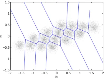
2.3. The MIMO Detection Problem 18 −2 −1.5 −1 −0.5 0 0.5 1 1.5 2 −1.5 −1 −0.5 0 0.5 1 1.5 y1 y2

Figure 2.4: MIMO 2×2 optimal decision regions.

and the SNR is 15 dB, through the 5 subfigures: a) shows the undistorted transmit constellation through antennas x1 and x2, b) the signals are rotated when the signal is

multiplied by the unitary matrix VH, c) the constellation is expanded or compressed according to the singular values σk along each axis, d) the resulting constellation in

rotated once more by the unitary matrix U, ande) shows the signal at the receiver after white Gaussian noise is added. Thus, the challenge for the receiver is to successfully determine what the transmitter sent, given that it receives a point as in Figure 2.3e). One of the simplest approaches for estimating the transmitted signal, is for the re-ceiver to reverse the steps that the MIMO channel performed. That is, de-rotate, ex-pand/compress, and de-rotate the constellation, since the receiver knows the channel

H. The result of this operation is shown in Fig. 2.3 f ), where it is seen that it has some resemblance to the transmitted signal in Figure 2.3 a), but the noise that was white becomes correlated, which causes detection errors when a decision is made. This detection approach is known as ZF and is one of the simplest detection methods, but one that usually achieves a poor error performance.

The difficulty of MIMO detection is related to finding the most probable vector that was transmitted, and this involves making a decision based on the closest point of the

(39)

2.3. The MIMO Detection Problem 19

distorted constellation. These regions are defined by the Voronoi diagram of the multi-dimensional constellation. This can be seen in Figure 2.4, where the optimal decision regions are plotted for possible received vectors. These regions can be very irregular and complex, especially for a high number of dimensions. The complexity of a MIMO detec-tion is related to the degree in which a particular algorithm is able to adjust its decision regions to the true Voronoi regions. It is well known that the algorithms that obtain an exact solution of (2.13) through exhaustive search, exhibit a complexity O(LK); that is, exponential in K and polynomial in L; in fact, (2.13) was proved to be NP-hard in [33]. Therefore, one of the main objectives of MIMO detection algorithm design is to find suboptimal methods with reduced complexity, while providing decision regions that approximate the optimal decision regions with a high degree of accuracy.

Another observation that can be made from Figure 2.3 c) is that when σmin is small,

the constellation points are compressed and become closer together, which increases the probability of performing an erroneous decision. As discussed in Section 2.2.1, high condition numbers are mostly due to the value of σmin being near zero. Therefore

in general, channel matrices with a high condition number κ incur in reduced error performance and increased detection complexity.

The MIMO detection problem is similar to the closest vector problem (CVP) in computer science, which amounts to finding the lattice point with the minimum Euclidean distance to a given input vector. CVP was been proved to be NP-hard in [34]. A lattice Λ is a arrangement of points in a periodic structure in multi-dimensional space. Formally, an infinite lattice is the structure generated by [35]

Λ(B) = Λ(b1,b2, ...,bn) ={Bx|x∈Zn} (2.15)

where Bis them×ngenerator matrix whose column vectors arebi, i∈ {1,2, ..., n} are

the basis vectors of Λ. The rank and dimension of Λ isnandm, respectively. For an ex-ample depiction, see Fig. 2.9 for a lattice with a generator matrixB= [ [1,1]T,[3,1]T].

(40)

2.4. Conventional MIMO Detection algorithms 20

In the context of MIMO detection, the basis vectors correspond to the column vectors of the channel matrix H, however, the lattices encountered are finite, which can present problems in certain cases [36].

2.4 Conventional MIMO Detection algorithms

This section provides a review of the most common ‘conventional’ MIMO detection algo-rithms. These detection techniques are usually associated with small-to-medium MIMO sizes (from approximately 2×2 through 20×20 antennas), and are the counterparts of the large MIMO detection algorithms, which will be discussed in Section 2.5. A charac-teristic of conventional MIMO detection techniques is that they suffer from an apparent tradeoff between error performance and computational complexity [37], as will be dis-cussed in this section. Conventional MIMO detection techniques have been extensively studied, a concise tutorial of how they work can be found in [10].

2.4.1 Optimal Detection Methods

ML Detection

As discussed previously, using the ML expression (2.13), the solution with the lowest possible error probability can be found through exhaustive search among all LK possi-ble transmit vectors for the one that provides the minimum value of the cost function. Although this is only practical for small MIMO systems, the algorithm is highly paral-lisable.

Sphere Decoder

An approach that reduces complexity compared to the full-search ML detector, while still providing optimum ML error performance is the sphere decoder (SD). The algorithm was first described by Fincke and Pohst [38], [39] and applied to fading channels by

(41)

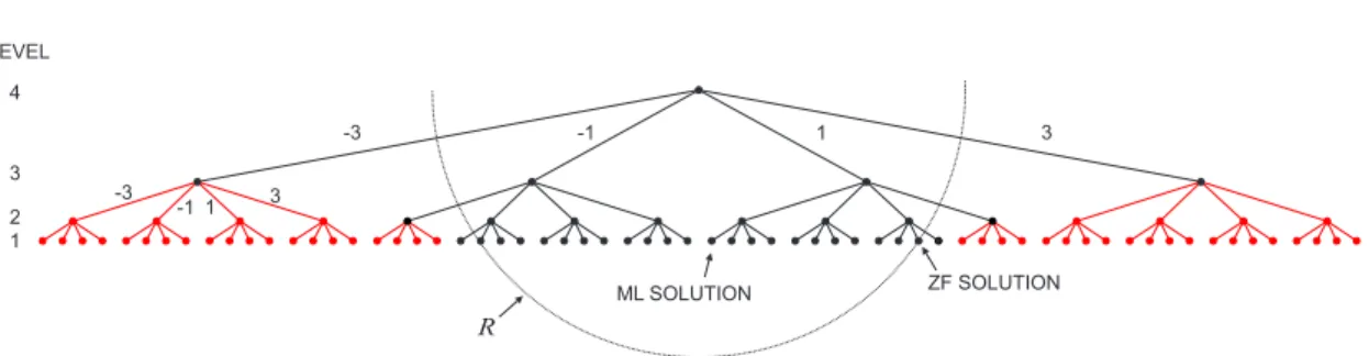
Figure 2.5: Conceptual diagram of the sphere decoder algorithm of a 4×4 MIMO system with 4-ABPSK modulation with constellation points {-3,-1,1,3}; R denotes the radius of the hypersphere.

Viterbo and Boutros [40]. An improved, less complex version was developed through the use of the Schnorr-Euchner (SE) enumeration [41], [35].

The algorithm works by representing the problem by a tree search, where each layer represents the possible values of the elements of x. Starting from an initial node, which could be obtained from a ZF decision, the algorithm then searches depth-first in a pre-defined fashion until it encounters a leaf node. It keeps track of the shortest distance R found so far of the leaf nodes encountered to the received vector as the search traverses the tree. The reduction in complexity is the result of skipping the search (pruning) for tree branches for nodes whose cumulative distance exceeds R. A conceptual diagram of the SD algorithm is found in Fig. 2.5, for a 4×4 MIMO system with 4-ABPSK modula-tion with constelamodula-tion points {−3,−1,1,3}. The red nodes and branches indicate those who would not be visited because their parent node exceeds R. A detailed algorithm can be found in [35].

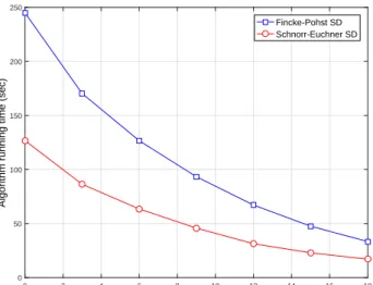
The average complexity of the Fincke-Pohst SD was found in [9] to be roughly cubic in K for moderate-to-high SNRs, however, the complexity is still exponential for low SNRs. Therefore, a disadvantage of the SD algorithm is that its complexity varies with the SNR. Fig. 2.6 shows an example algorithm running time vs. SNR for the Fincke-Pohst and Schnorr-Euchner variants of the SD algorithm. From the figure, the decrease in complexity is evident as the SNR increases. Furthermore, it can be observed that the running time for the Schnorr-Euchner approach is roughly half of that of its counterpart.

(42)

2.4. Conventional MIMO Detection algorithms 22 0 2 4 6 8 10 12 14 16 18 SNR (dB) 0 50 100 150 200 250

Algorithm running time (sec)

Fincke-Pohst SD Schnorr-Euchner SD

Figure 2.6: Example sphere decoding algorithm running time vs. SNR for the Fincke-Pohst and Schnorr-Euchner variants.

The fixed-complexity sphere decoder (FCSD) [42] is based on SD, it performs full search for the top specified layers of the tree, and uses a decision feedback equaliser (DFE) for the rest of the layers. FCSD exhibits fixed complexity throughout the SNR range, however, it comes at the cost of losing BER optimality, and it is still too complex when the MIMO size is large [23].

The SD algorithm can be modified to output soft detection decisions, as in the list sphere decoder (LSD) [43] for use in forward error correction (FEC) coded systems. Soft decisions are obtained through the log-likelihood ratio (LLR) [44]

L(bi|y) = log P(bi= 1)|y P(bi= 0)|y = log     P x:bi(x)=1 exp −σ_v−2ky−Hxk2 P x:bi(x)=0 exp −σv−2ky−Hxk2     , i∈[1, Klog₂L] (2.16)

where the notationbi, i∈[1, Klog2L] refers to thei-th bit contained in the transmitted

vector x, and the notation (x :bi(x) = a) is the set of all vectors x for which bi =a.

(43)

which makes it feasible only when there are a small number of UTs.

An approximation of (2.16) consists on performing the summations over a smaller subset of vectors, and is the principle of the LSD, where the subset V of vectors considered are only the ones that lie within the hypersphere defined by its radius R. While this approach is less complex than the full search approach in (2.16), it still incurs in increased complexity compared to the hard decision SD, since the radius R needs to be kept large enough so that V contains a large number of vectors in order to obtain a close approximation to the true LLR.

Approximate ML BER

Due to its error performance optimality, the ML BER serves as the standard to which other detectors are evaluated in their error rate results. Unfortunately, an analytical closed form expression for the ML BER is not available. However, a useful approximation exists based on the pairwise error probability (PEP), which is the probability that the estimated symbol ˆxk is erroneously detected, therefore ˆxk 6= xk (see (2.34)); and for

quadrature phase shift keying (QPSK), the ML BER approximation is given by [45]

P_ML≈Q(√αML·γo) , (2.17)

where Q(·) is the Q-function. When the channel is i.i.d. complex Gaussian, αML is a

chi-square (X2_{)-distributed random variable with 2}_M _DoF.

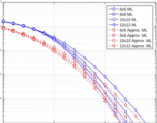
In order to observe the tightness of the BER approximation in (2.17) to the true BER of an ML detector, Fig. 2.7 compares the ML BER obtained from a SD against (2.17) for MIMO sizes of 6 ×6, 8×8, 10×10, and 12×12 antennas. From the figure, it can be observed that the ML and approximate ML curves become closer as the SNR grows. Furthermore, the approximation becomes tighter as the MIMO size increases. This approximation will be useful for the BER analysis in Chapter 4.

(44)

2.4. Conventional MIMO Detection algorithms 24 0 5 10 15 Eb/N0 (dB) 10-4 10-3 10-2 10-1 100 Average BER 6x6 ML 8x8 ML 10x10 ML 12x12 ML 6x6 Approx. ML 8x8 Approx. ML 10x10 Approx. ML 12x12 Approx. ML

Figure 2.7: True ML vs. ML approximation in (2.17) for an i.i.d. flat Rayleigh fading channel, for different MIMO sizes.

2.4.2 Linear Detection

Linear detection methods, MF, ZF and linear MMSE are the simplest for MIMO. The ZF equaliser or decorrelator is basically the pseudoinverse of the channel matrix

WZF =H†= HHH

−1

HH (2.18)

where (·)† and (·)H denote the matrix pseudoinversion operation and the complex con-jugate transpose operation, respectively. Applying the equaliser WZF to (2.1)

ˆ

x=H†y=x+H†v=x+ ˜v (2.19)

completely removes interference. However, the noise that was uncorrelated in v be-comes correlated in ˜v. This can severely affect the performance, especially for channel realisations with an ill-conditioned matrix.

(45)

very low SNR, the MF WMF =HH equaliser performs best as it maximises the signal

without regard for interference. When applied to the received signal, the result is

ˆ

x=WMFy =HHH x+HHv, (2.20)

where it is clear that the recovered signals would suffer substantial interference, unless

HH_H_{closely resembles a diagonal matrix.}

The overall optimal linear equaliser is the result of finding the equaliserWthat minimises the mean square error (MSE) [46] [21]

MSE=EkWy−xk2 (2.21)

the result is the MMSE equaliser and it is given by [21, Sec. 8.3.3]

WMMSE= HHH+γo−1I

−1

HH (2.22)

The MMSE filter takes noise into consideration to provide a balance between interference and noise.

In the context of detection for large MIMO systems, ZF and MMSE receivers are attrac-tive because of their relaattrac-tively low complexity, but the maximum diversity order they provide when the modulation is complex-valuedb isM−K+ 1 [47], which results in low error performance when the number of transmit and receive antennas is approximately equal.

2.4.3 Widely-Linear Processing

In communication networks, widely linear (WL) processing achieves superior perfor-mance over strictly linear filters when the transmission signal, interference or noise is

b

(46)

improper (or second-order noncircular [48]) [49], that is, their pseudo-covariance matrix is non-vanishing. In other words, it means that for complex random processes, the real and imaginary components have different second-order statistics.

Examples of proper random processes include the circularly symmetric onesc (such as AWGN), and multilevel quadrature amplitude modulation (QAM); whereas examples of

improper random processes include rectangular QAM, multilevel ABPSK, and coloured noise.

For a complex-valued multivariate random variable x = xI+jxQ, where xI = R(x)

and xQ =I(x) are the in-phase and quadrature components, respectively, the

pseudo-covariance matrix Jis defined as [21, eq. A.16]

J,E[(x−µ)(x−µ)T], (2.23)

where µ=E[x].

Denote y = yI + jyQ, where yI = R(y) and yQ = I(y) to be a linear function of x. The interest is in finding an estimate ˆx of x, given that y is observed. Since for improper signals J 6= 0, the covariances of xI and xQ are different, therefore a single

MMSE filterWMMSEcannot be simultaneously optimal for estimating both the in-phase

and quadrature components ofx. The solution is to use two distinct complex filters WI

and WQ, foryI and yQ, respectively. Therefore, the estimate of xbecomes (e.g. [50])

ˆ

x=WH_I yI+WHQyQ (2.24)

=FH₁ y+FH₂ y∗, (2.25)

where F1 =WI+WQ, F2 =WI−WQ, and (·)∗ is the complex conjugate operator.

It is worthwhile noting that when x is proper, WI = WQ, and F2 =0; consequently,

(2.25) reduces to the strictly linear filter form.

WL processing techniques have been proven useful and relevant to numerous

(47)

tions. Particularly, WL techniques of have been applied in [51], [52], and [24] when using real-valued transmitted signals, such as binary phase shift keying (BPSK) and ABPSK, by exploiting their improperness. Furthermore, since Gaussian minimum shift keying (GMSK) modulation can be approximated by filtered BPSK [53], WL filtering has proposed for global system for mobile communication (GSM) networks, particularly for single antenna interference cancellation (SAIC) [54], [55], [53]. Additional applica-tions are in orthogonal frequency-division multiplexing (OFDM) [56], SISO systems with adaptive constellations [57], CDMA [58], [59], and in multiple-antenna systems, includ-ing: V-BLAST spatial multiplexing [24], [60], space-time codes (STC) [61], [62], [55], and MIMO models [51].

2.4.4 Real-Valued Modulation and ABPSK

A recurring theme in this thesis is the assertion that the use of real-valued modulations in MU-MIMO increases the spatial diversity of MU-MIMO and consequently allow the use of low-complexity detectors. As a special case of real constellations, the one used throughout this work is perhaps the simplest case where there the constellation points are placed along the real axis, with equal spacing between adjacent points, and these can be positive or negative; a representation is shown on the right side of Fig. 2.8. There is, however, an ambiguity regarding the name of this modulation type. Some authors refer to it as multilevel PAM (M-PAM) (see, e.g. [63], [21], [64], [44]), while other authors refer to it as multilevel amplitude shift keying (ASK) in [24], and [65] (where it is also referred to as multiple amplitude modulation (M-AM)). However, ASK usually denotes another type of modulation where the amplitude of the carrier is used to represent the digital signal [66], whereas PAM often refers to a modulation scheme that represents the analog data as the amplitude of a series of regularly-timed pulses [67]. To avoid confusion, we refer to the digital modulation scheme described above as L-ary amplitude binary-phase shift keying (ABPSK). A depiction of a 4-ABPSK constellation is shown in Fig. 2.8 (right), and a 16-QAM constellation on the left of the same figure

(48)

Figure 2.8: 16-QAM constellation (left), and 4-ABPSK constellation (right), where a denotes the amplitude factor, I and Q the inline and quadrature axes, respectively.

as reference.

2.4.5 Successive Interference Cancellation

The SIC MIMO detection approach was proposed in [13], where it is named as V-BLASTd. The algorithm works by estimating one element of the transmit vector at one time, usually starting with the one with the highest post-equalisation SNR or signal-to-interference-plus-noise ratio (SINR), then subtracting its effect from the remaining non-estimated signal and iterating until all elements are detected. The reason for first detecting the strongest elements is to avoid error propagation, since once an estimation error is made, all further elements will likely be incorrect as well.

Either ZF or MMSE (referred to as ZF-SIC and MMSE-SIC, respectively) can be used as the equaliser for SIC, and the detection sequence or ordering can be determined once for each channel realisation based on the post-equalisation SNR or SINR of each stream, for ZF-SIC and MMSE-SIC, respectively. Specifically for MMSE-SIC, the stream that

d

This term is also often used to describe the MIMO architecture where individual data streams are coded and transmitted, which is also the scenario considered in this thesis. However, here the term refers to the detection method.

(49)

should be canceled at each iteration is the one with the highest post-equalisation SINR, given by [68] SINRk= σ_x2 |wMMSE,khk|2 σ2 x P k6=j|wMMSE,khj| 2 +σ2 v kwMMSE,kk2 , k∈[1, K], (2.26)

where MMSE, k refers to the k-th row of the equalisation matrix given in (2.22). Sim-ilarly, for ZF-SIC, the selected stream to be canceled at each iteration is the one with the highest post-equalisation SNR, which is [68]

SNRk=

σ_x2 σ2

v kwZF,kk2

, k∈[1, K], (2.27)

where wZF,k is thek-th row of the ZF equaliser given in (2.18). It should be noted that

since σ_x2 and σ_v2 do not depend on k, it suffices to choose the index of the row of wZF,k

with the lowest norm, which is the approach used in the original SIC paper [13]. It should be noted that the overall optimal ordering is dependent on the received vector, but doing this would incur in a high computation cost [68].

The original algorithm by [13] has O(K4) complexity. But by reducing redundant op-erations, mainly by avoiding performing channel matrix inversion on every iteration, complexity is reduced to O(K3) in [69] and [70].

The SIC technique provides a good balance between error performance and algorithm complexity.

2.4.6 Lattice Reduction

In general, ill-conditioned channel matrices are harder to estimate without errors. This is because typically such matrices have a large orthogonality defect (OD), which is defined as [11] δ(B) = Π K i=1||bi|| p det(BH_B₎, (2.28)

(50)

Figure 2.9: Lattice generated by the basis B = [ [1,1]T,[3,1]T ], and the basis after reduction ˜B= [ [1,1]T,[−1,1]T ], which has a lower orthogonality defect.

where B refers to the basis of the lattice, as defined in (2.15)e.

LR techniques can provide a ‘lattice-reduced’ matrix ˜H=HTwith a lower OD. T is a unimodular matrix, i.e. its elements are integers and det(T) =±1.

Once ˜H has been computed, an equivalent system model is found and detection can progress using a conventional approach such as ZF, MMSE or SIC

y=Hx+v=HTT−1x+v (2.29)

y= ˜Hz˜+v, (2.30)

where ˜z=T−1x.

e

We use the notation B to refer to the bases of general lattices, whereas we use H in MU-MIMO communication contexts. The main difference is that in MU-MIMO, the lattices encountered are finite.